
Machine Learning-Based Peripheral Artery Disease Identification Using Laboratory-Based Gait Data

 ,
,  , ,
, , 
 and
and 
Abstract
1. Introduction
2. Data Sources
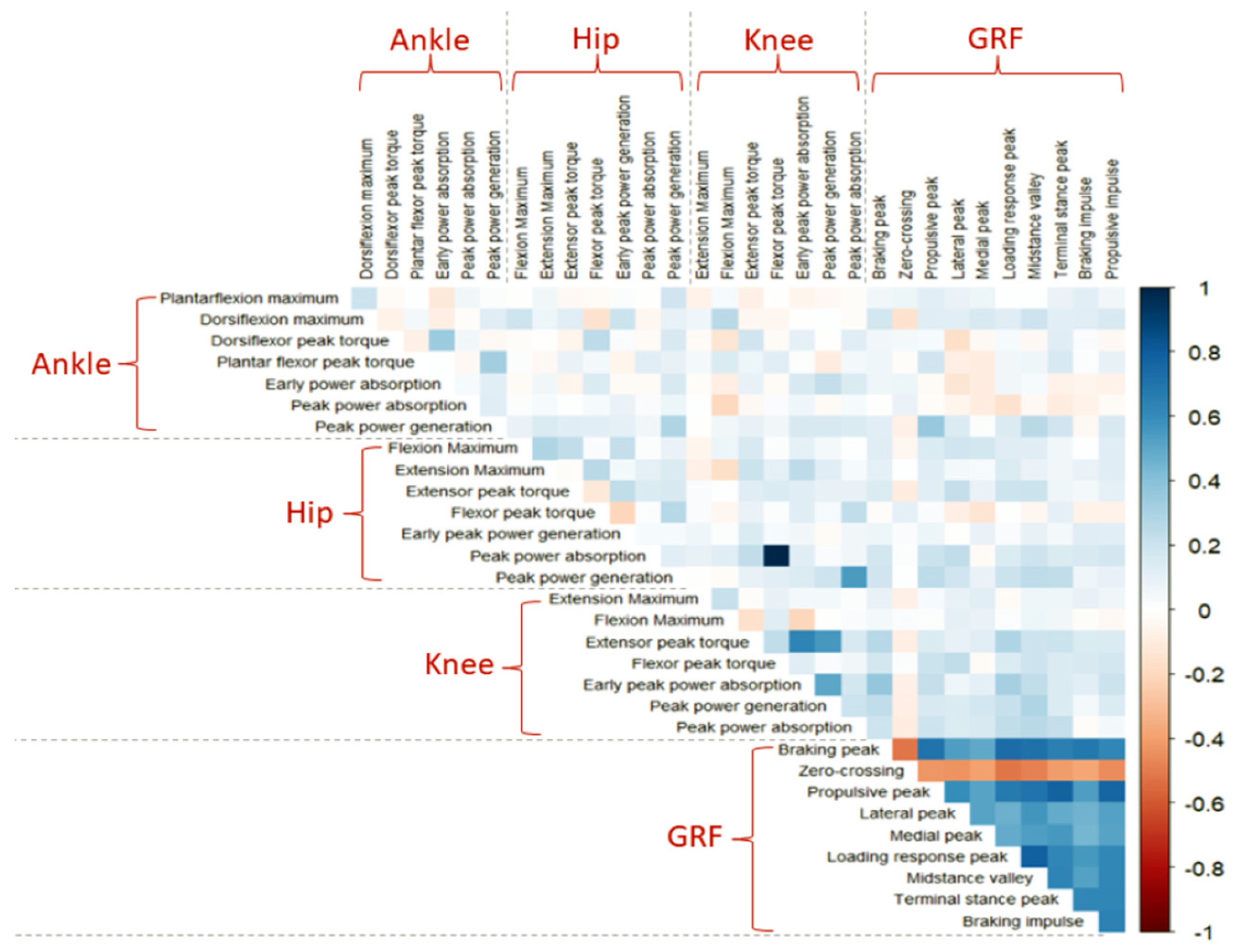
3. Descriptive Data Analysis
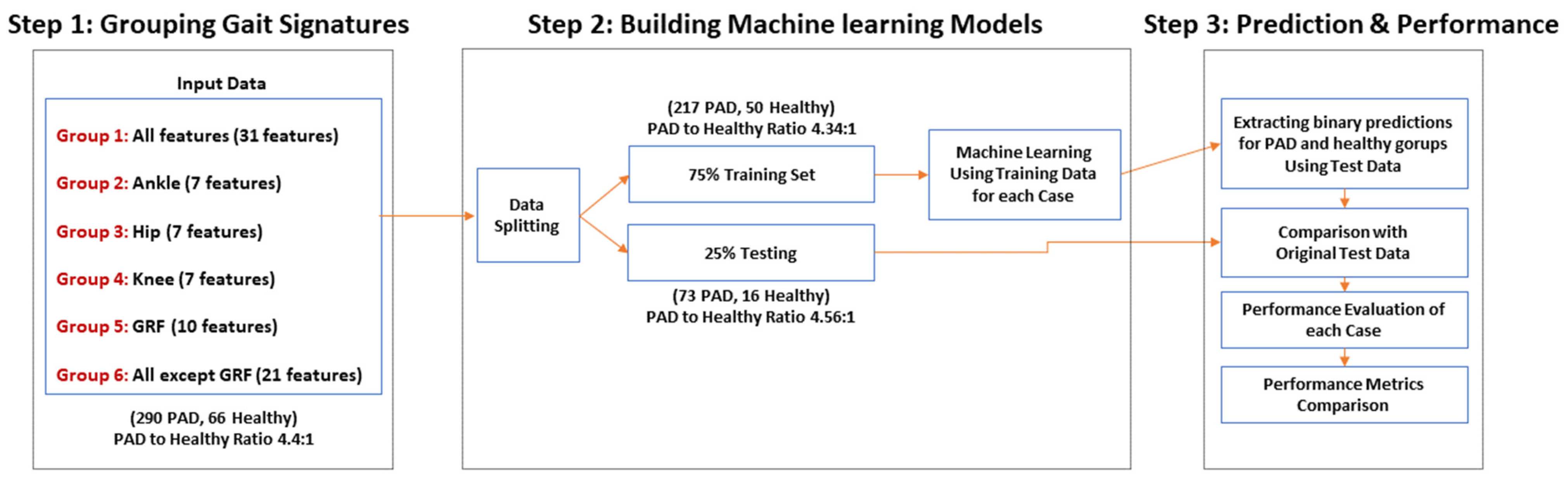
4. Predictive ML Models to Diagnose PAD
5. ML Models Results
6. Discussion
7. Conclusions
Supplementary Materials
Author Contributions
Funding
Institutional Review Board Statement
Informed Consent Statement
Data Availability Statement
Conflicts of Interest
Appendix A

| Gait Feature Source | Raw Signal | Gait Signature Extracted | Definition and Explanation |
|---|---|---|---|
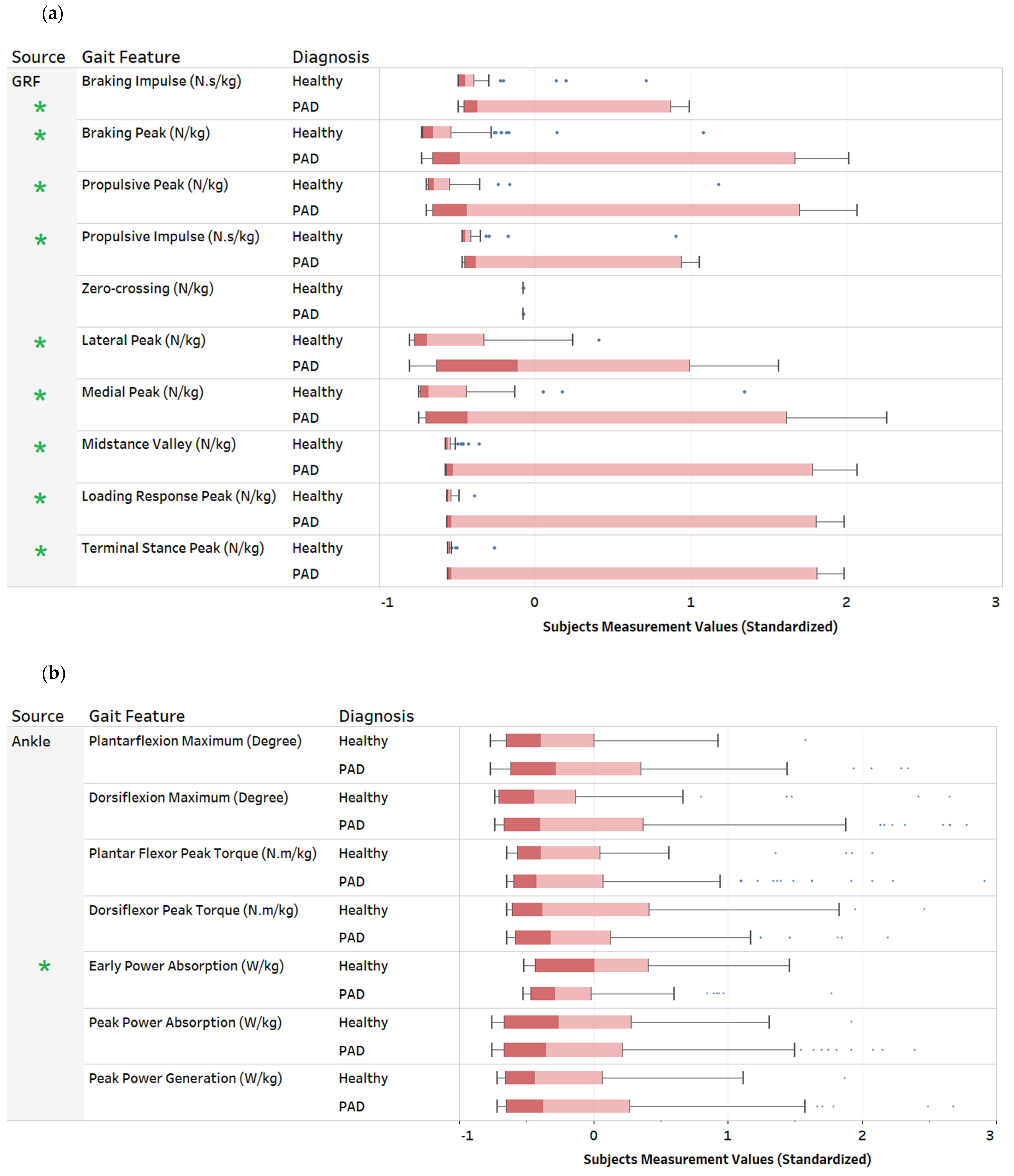
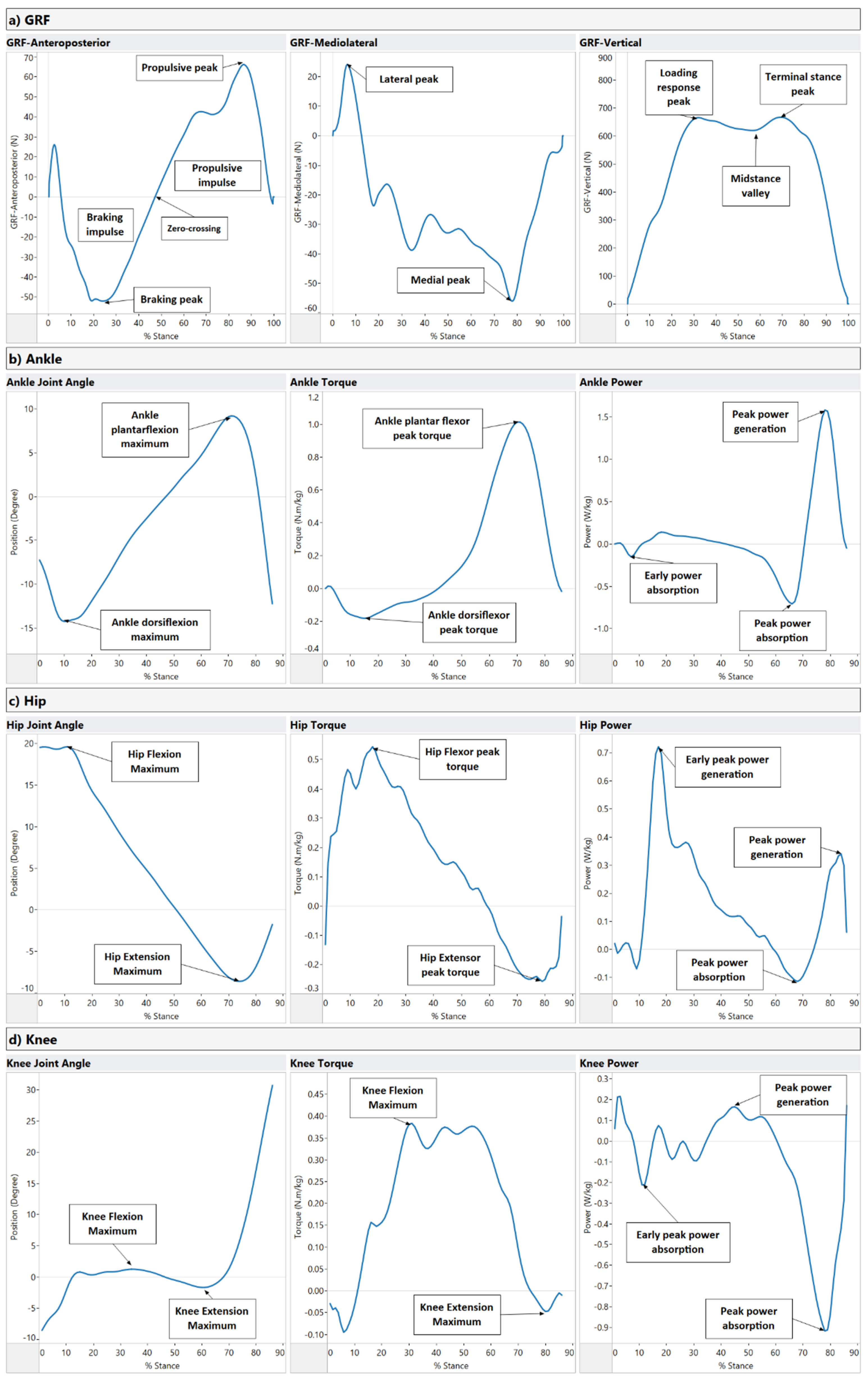
| Ground Reaction Forces (GRF) Figure A1a | GRF x-axis (Anteroposterior component) | Braking peak: Initial negative force component after heel contact. (N/kg) Zero-crossing: the midpoint of the anteroposterior component. (N/kg) Propulsive peak: The positive peak of the propulsion component. (N/kg) Braking impulse: The area under the anterior-posterior force curve between touch-down and zero-crossing at midstance. (N.s/kg) Propulsive impulse: The area under the anterior-posterior force curve between zero-crossing at midstance and toe-off. (N.s/kg) | GRF is recorded on overground force plates, where the center of pressure is expressed in a standard cartesian coordinate system (x, y, z). The ground reaction force is exerted by the ground on a body in contact with it and is composed of three components: vertical, anterior-posterior, and mediolateral. These forces can be combined with the limb orientation data to calculate ankle, knee, and hip joint torques and powers. The rotating effect of the force located at a distance from the joint axis is quantified using joint torques, while the joint power quantifies the power output of individual joints during walking. |
| GRF y-axis (Mediolateral component) | Lateral peak: The maximum short positive force component immediately after heel contact. (N/kg) Medial peak: The minimum negative force component as the foot snatches for toe-off. (N/kg) | ||
| GRF z-axis (Vertical component) | Loading response peak: Rapid rise in force after heel contact. (N/kg) Midstance valley: The minimum force exerted by the center of mass at midstance. (N/kg) Terminal stance peak: Second peak force that is greater than body weight (N/kg) | ||
| Ankle Figure A1b | Ankle Joint Angle | Ankle plantarflexion maximum: Peak plantarflexion during stance. (Degree) Ankle dorsiflexion maximum: Peak dorsiflexion during stance. (Degree) | The ankle is plantar flexed at heel strike in the range of 5–6 degrees, moves to 10–12 degrees of dorsiflexion, and then back to plantarflexion (15–20 degrees) at toe-off. |
| Ankle Torque | Ankle dorsiflexor peak torque: Peak response of the ankle dorsi flexors during stance. (N.m/kg) Ankle plantar flexor peak torque: Peak response of the ankle plantar flexors (extensors) during stance. (N.m/kg) | During loading, the ankle has a dorsiflexor torque as the foot is lowered to the ground. Next, a plantarflexion torque occurs through midstance to control the weight transfer over the ankle as the body moves over the foot. Finally, at late stance, the plantarflexion torque continues as the plantar flexors advance the foot into the swing. | |
| Ankle Power | Early power absorption: (Eccentric muscular contraction) at the ankle after heel strike. (W/kg) Peak power absorption: (Eccentric muscular contraction) at the ankle during midstance. (W/kg) Peak power generation: (Concentric muscular contraction) at the ankle during late stance. (W/kg) | At loading response, power is absorbed by the dorsiflexors as the foot is lowered to the ground. Power absorption continues by the plantar flexors as the body moves over the foot. Finally, power is generated by the plantar flexors to drive the leg into the swing. | |
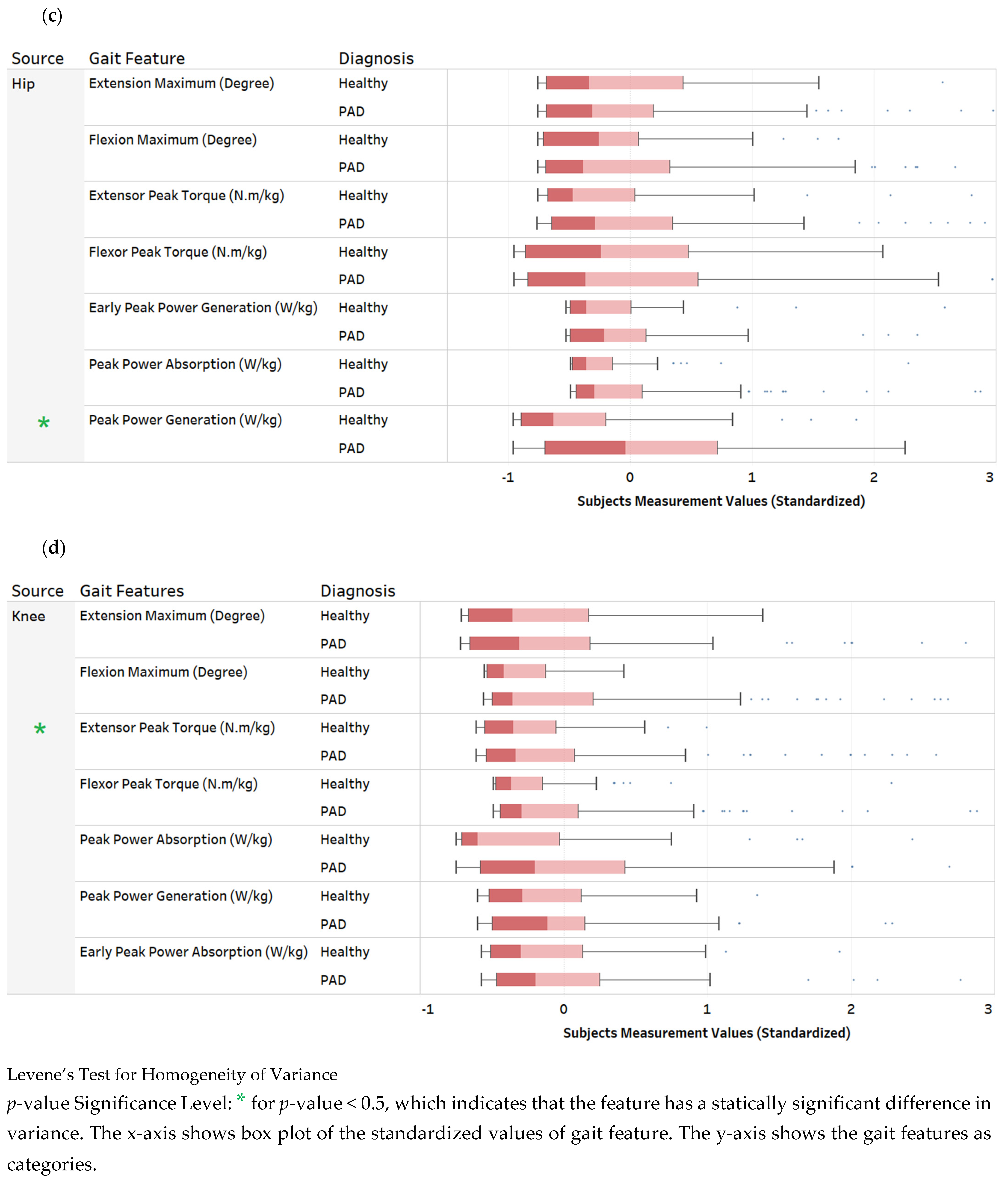
| Hip Figure A1c | Hip Joint Angle | Hip Flexion Maximum: Peak hip flexion during stance. (Degree) Hip Extension Maximum: Peak hip extension during stance. (Degree) | Peak hip flexion usually occurs at heel contact and is approximately 35–50 degrees. After heel contact, hip flexion reduces throughout support until toe-off. |
| Hip Torque | Hip Flexor peak torque: Peak response of the hip flexors during stance. (N.m/kg) Hip Extensor peak torque: Peak response of the hip extensors during stance. (N.m/kg) | A net hip extensor torque during the initial loading phase of support continues through midstance into late stance. | |
| Hip Power | Early peak power generation: (Concentric muscular contraction) at the hip after heel strike. (W/kg) Peak power absorption: (Eccentric muscular contraction) at the hip during midstance. (W/kg) Peak power generation: (Concentric muscular contraction) at the hip during late stance. (W/kg) | At heel contact, there is power generation of the hip extensors. In late stance, there is new power absorption by the hip extensors to decelerate the hip flexors, followed by power generation of the hip flexors to propel the leg into the swing. | |
| Knee Figure A1d | Knee Joint Angle | Knee Flexion Maximum: Peak dorsiflexion during stance. (Degree) Knee Extension Maximum: Peak plantarflexion during stance. (Degree) | The ankle is plantar flexed at heel strike in the range of 5–6 degrees and moves to 10–12 degrees of dorsiflexion and then back to plantarflexion (15–20 degrees) at toe-off. |
| Knee Torque | Knee Flexor peak torque: Peak response of the knee flexors during stance. (N.m/kg) Knee Extensor peak torque: Peak response of the knee extensors during stance. (N.m/kg) | The loading response at the knee involves an extensor torque of the knee, which transfers to a flexor torque after the knee angle moves into extension towards toe-off. | |
| Knee Power | Early peak power absorption: (Concentric muscular contraction) at the knee after heel strike. (W/kg) Peak power generation: (Concentric muscular contraction) at the knee during mid stance. (W/kg) Peak power absorption: (Eccentric muscular contraction) at the knee during terminal stance. (W/kg) | There is knee flexion controlled by the extensors (power absorption) at heel contact moving into midstance, where there is a knee extensor torque controlled by the extensors (power generation). In late stance, there is a knee extensor torque controlled by the extensors (power generation). |

References
- Dhaliwal, G.; Mukherjee, D. Peripheral Arterial Disease: Epidemiology, Natural History, Diagnosis and Treatment. Int. J. Angiol. 2007, 16, 36. [Google Scholar] [CrossRef] [PubMed]
- Nehler, M.R.; Duval, S.; Diao, L.; Annex, B.H.; Hiatt, W.R.; Rogers, K.; Zakharyan, A.; Hirsch, A.T. Epidemiology of Peripheral Arterial Disease and Critical Limb Ischemia in an Insured National Population. J. Vasc. Surg. 2014, 60, 686–695.e2. [Google Scholar] [CrossRef] [PubMed]
- Matsushita, K.; Sang, Y.; Ning, H.; Ballew, S.H.; Chow, E.K.; Grams, M.E.; Selvin, E.; Allison, M.; Criqui, M.; Coresh, J.; et al. Lifetime Risk of Lower-Extremity Peripheral Artery Disease Defined by Ankle-Brachial Index in the United States. J. Am. Heart Assoc. 2019, 8, e012177. [Google Scholar] [CrossRef] [PubMed]
- Allison, M.A.; Ho, E.; Denenberg, J.O.; Langer, R.D.; Newman, A.B.; Fabsitz, R.R.; Criqui, M.H. Ethnic-Specific Prevalence of Peripheral Arterial Disease in the United States. Am. J. Prev. Med. 2007, 32, 328–333. [Google Scholar] [CrossRef] [PubMed]
- Song, P.; Rudan, D.; Zhu, Y.; Fowkes, F.J.I.; Rahimi, K.; Fowkes, F.G.R.; Rudan, I. Global, Regional, and National Prevalence and Risk Factors for Peripheral Artery Disease in 2015: An Updated Systematic Review and Analysis. Lancet Glob. Health 2019, 7, e1020–e1030. [Google Scholar] [CrossRef]
- Fowkes, F.G.R.; Rudan, D.; Rudan, I.; Aboyans, V.; Denenberg, J.O.; McDermott, M.M.; Norman, P.E.; Sampson, U.K.A.; Williams, L.J.; Mensah, G.A.; et al. Comparison of Global Estimates of Prevalence and Risk Factors for Peripheral Artery Disease in 2000 and 2010: A Systematic Review and Analysis. Lancet 2013, 382, 1329–1340. [Google Scholar] [CrossRef]
- Kithcart, A.P.; Beckman, J.A. ACC/AHA Versus ESC Guidelines for Diagnosis and Management of Peripheral Artery Disease. J. Am. Coll. Cardiol. 2018, 72, 2789–2801. [Google Scholar] [CrossRef]
- Murabito, J.M.; D’Agostino, R.B.; Silbershatz, H.; Wilson, P.W.F. Intermittent Claudication: A Risk Profile from the Framingham Heart Study. Circulation 1997, 96, 44–49. [Google Scholar] [CrossRef]
- Vogt, M.T. Decreased Ankle/Arm Blood Pressure Index and Mortality in Elderly Women. JAMA J. Am. Med. Assoc. 1993, 270, 465. [Google Scholar] [CrossRef]
- Rose, G.A.; Blackburn, H.; Gillum, R.F.; Prineas, R.J. Cardiovascular Survey Methods. World Health Organ. Monogr. Ser. 1982, 56, 188. [Google Scholar]
- Meru, A.V.; Mittra, S.; Thyagarajan, B.; Chugh, A. Intermittent Claudication: An Overview. Atherosclerosis 2006, 187, 221–237. [Google Scholar] [CrossRef] [PubMed]
- Norgren, L.; Hiatt, W.R.; Dormandy, J.A.; Nehler, M.R.; Harris, K.A.; Fowkes, F.G.R.; Bell, K.; Caporusso, J.; Durand-Zaleski, I.; Komori, K.; et al. Inter-Society Consensus for the Management of Peripheral Arterial Disease (TASC II). Eur. J. Vasc. Endovasc. Surg. 2007, 33, S1–S75. [Google Scholar] [CrossRef] [PubMed]
- Regensteiner, J.G.; Hiatt, W.R.; Coll, J.R.; Criqui, M.H.; Treat-Jacobson, D.; McDermott, M.M.; Hirsch, A.T.; Rooke, T. The Impact of Peripheral Arterial Disease on Health-Related Quality of Life in the Peripheral Arterial Disease Awareness, Risk, and Treatment: New Resources for Survival (PARTNERS) Program. Vasc. Med. 2008, 13, 15–24. [Google Scholar] [CrossRef] [PubMed]
- Gardner, A.W.; Montgomery, P.S. The Relationship between History of Falling and Physical Function in Subjects with Peripheral Arterial Disease. Vasc. Med. 2001, 6, 223–227. [Google Scholar] [CrossRef] [PubMed]
- McDermott, M.M.G.; Ohlmiller, S.M.; Liu, K.; Guralnik, J.M.; Martin, G.J.; Pearce, W.H.; Greenland, P. Gait Alterations Associated with Walking Impairment in People with Peripheral Arterial Disease with and without Intermittent Claudication. J. Am. Geriatr. Soc. 2001, 49, 747–754. [Google Scholar] [CrossRef]
- Feinglass, J.; McCarthy, W.J.; Slavensky, R.; Manheim, L.M.; Martin, G.J.; Keen, R.; Govostis, D.M.; Golan, J.F.; Schneider, J.R.; Madayag, M.; et al. Effect of Lower Extremity Blood Pressure on Physical Functioning in Patients Who Have Intermittent Claudication. J. Vasc. Surg. 1996, 24, 503–512. [Google Scholar] [CrossRef]
- Issa, S.M.; Hoeks, S.E.; Reimer, W.J.S.O.; Van Gestel, Y.R.B.M.; Lenzen, M.J.; Verhagen, H.J.M.; Pedersen, S.S.; Poldermans, D. Health-Related Quality of Life Predicts Long-Term Survival in Patients with Peripheral Artery Disease. Vasc. Med. 2010, 15, 163–169. [Google Scholar] [CrossRef]
- Myers, S.A.; Applequist, B.C.; Huisinga, J.M.; Pipinos, I.I.; Johanning, J.M. Gait Kinematics and Kinetics Are Affected More by Peripheral Arterial Disease than by Age. J. Rehabil. Res. Dev. 2016, 53, 229–238. [Google Scholar] [CrossRef]
- Myers, S.A.; Johanning, J.M.; Pipinos, I.I.; Schmid, K.K.; Stergiou, N. Vascular Occlusion Affects Gait Variability Patterns of Healthy Younger and Older Individuals. Ann. Biomed. Eng. 2013, 41, 1692–1702. [Google Scholar] [CrossRef]
- Wurdeman, S.R.; Koutakis, P.; Myers, S.A.; Johanning, J.M.; Pipinos, I.I.; Stergiou, N. Patients with Peripheral Arterial Disease Exhibit Reduced Joint Powers Compared to Velocity-Matched Controls. Gait Posture 2012, 36, 506–509. [Google Scholar] [CrossRef]
- McDermott, M.M.; Kerwin, D.R.; Liu, K.; Martin, G.J.; O’Brien, E.; Kaplan, H.; Greenland, P. Prevalence and Significance of Unrecognized Lower Extremity Peripheral Arterial Disease in General Medicine Practice. J. Gen. Intern. Med. 2001, 16, 384–390. [Google Scholar] [CrossRef] [PubMed]
- Clairotte, C.; Retout, S.; Potier, L.; Roussel, R.; Escoubet, B. Automated Ankle-Brachial Pressure Index Measurement by Clinical Staff for Peripheral Arterial Disease Diagnosis in Nondiabetic and Diabetic Patients. Diabetes Care 2009, 32, 1231–1236. [Google Scholar] [CrossRef] [PubMed]
- Firnhaber, J.M.; Carolina, M.A.; Daop, N. Lower Extremity Peripheral Artery Disease: Diagnosis and Treatment. Am. Fam. Physician 2019, 99, 362–369. [Google Scholar]
- Simon, A.; Papoz, L.; Ponton, A.; Segond, P.; Becker, F.; Drouet, L.; Levenson, J.; Marazanof, M.; Sentou, Y.; Chollet, E.; et al. Feasibility and Reliability of Ankle/Arm Blood Pressure Index in Preventive Medicine. Angiology 2000, 51, 463–471. [Google Scholar] [CrossRef]
- Sheng, C.-S.; Li, Y.; Huang, Q.-F.; Kang, Y.-Y.; Li, F.-K.; Wang, J.-G. Pulse Waves in the Lower Extremities as a Diagnostic Tool of Peripheral Arterial Disease and Predictor of Mortality in Elderly Chinese. Hypertension 2016, 67, 527–534. [Google Scholar] [CrossRef]
- Donohue, C.M.; Adler, J.V.; Bolton, L.L. Peripheral Arterial Disease Screening and Diagnostic Practice: A Scoping Review. Int. Wound J. 2020, 17, 32–44. [Google Scholar] [CrossRef]
- Ramirez, J.L.; Magaret, C.A.; Khetani, S.A.; Rhyne, R.F.; Peters, C.; Barnes, G.; Grenon, S.M. PC102. A Novel Machine Learning-Driven Clinical and Proteomic Tool for the Diagnosis of Peripheral Artery Disease. J. Vasc. Surg. 2019, 69, e233–e234. [Google Scholar] [CrossRef]
- Ross, E.G.; Shah, N.H.; Dalman, R.L.; Nead, K.T.; Cooke, J.P.; Leeper, N.J. The Use of Machine Learning for the Identification of Peripheral Artery Disease and Future Mortality Risk. J. Vasc. Surg. 2016, 64, 1515–1522.e3. [Google Scholar] [CrossRef]
- Baloch, Z.O.; Raza, S.A.; Pathak, R.; Marone, L.; Ali, A. Machine Learning Confirms Nonlinear Relationship between Severity of Peripheral Arterial Disease, Functional Limitation and Symptom Severity. Diagnostics 2020, 10, 515. [Google Scholar] [CrossRef]
- Kim, S.; Hahn, J.-O.; Youn, B.D. Detection and Severity Assessment of Peripheral Occlusive Artery Disease via Deep Learning Analysis of Arterial Pulse Waveforms: Proof-of-Concept and Potential Challenges. Front. Bioeng. Biotechnol. 2020, 8, 720. [Google Scholar] [CrossRef]
- Flores, A.M.; Demsas, F.; Leeper, N.J.; Ross, E.G. Leveraging Machine Learning and Artificial Intelligence to Improve Peripheral Artery Disease Detection, Treatment, and Outcomes. Circ. Res. 2021, 128, 1833–1850. [Google Scholar] [CrossRef] [PubMed]
- Ara, L.; Luo, X.; Sawchuk, A.; Rollins, D. Automate the Peripheral Arterial Disease Prediction in Lower Extremity Arterial Doppler Study Using Machine Learning and Neural Networks. In Proceedings of the 10th ACM International Conference on Bioinformatics, Computational Biology and Health Informatics, Niagara Falls, NY, USA, 4 September 2019; ACM: New York, NY, USA, 2019; pp. 130–135. [Google Scholar]
- Horst, F.; Lapuschkin, S.; Samek, W.; Müller, K.-R.; Schöllhorn, W.I. Explaining the Unique Nature of Individual Gait Patterns with Deep Learning. Sci. Rep. 2019, 9, 2391. [Google Scholar] [CrossRef] [PubMed]
- Li, M.H.; Mestre, T.A.; Fox, S.H.; Taati, B. Vision-Based Assessment of Parkinsonism and Levodopa-Induced Dyskinesia with Pose Estimation. J. Neuroeng. Rehabil. 2018, 15, 97. [Google Scholar] [CrossRef]
- Kondragunta, J.; Wiede, C.; Hirtz, G. Gait Analysis for Early Parkinson’s Disease Detection Based on Deep Learning. Curr. Dir. Biomed. Eng. 2019, 5, 9–12. [Google Scholar] [CrossRef]
- Juutinen, M.; Wang, C.; Zhu, J.; Haladjian, J.; Ruokolainen, J.; Puustinen, J.; Vehkaoja, A. Parkinson’s Disease Detection from 20-Step Walking Tests Using Inertial Sensors of a Smartphone: Machine Learning Approach Based on an Observational Case-Control Study. PLoS ONE 2020, 15, e0236258. [Google Scholar] [CrossRef] [PubMed]
- Schieber, M.N.; Pipinos, I.I.; Johanning, J.M.; Casale, G.P.; Williams, M.A.; DeSpiegelaere, H.K.; Senderling, B.; Myers, S.A. Supervised Walking Exercise Therapy Improves Gait Biomechanics in Patients with Peripheral Artery Disease. J. Vasc. Surg. 2020, 71, 575–583. [Google Scholar] [CrossRef]
- Myers, S.A.; Pipinos, I.I.; Johanning, J.M.; Stergiou, N. Gait Variability of Patients with Intermittent Claudication Is Similar before and after the Onset of Claudication Pain. Clin. Biomech. 2011, 26, 729–734. [Google Scholar] [CrossRef]
- Szymczak, M.; Krupa, P.; Oszkinis, G.; Majchrzycki, M. Gait Pattern in Patients with Peripheral Artery Disease. BMC Geriatr. 2018, 18, 52. [Google Scholar] [CrossRef]
- Crowther, R.G.; Spinks, W.L.; Leicht, A.S.; Quigley, F.; Golledge, J. Relationship between Temporal-Spatial Gait Parameters, Gait Kinematics, Walking Performance, Exercise Capacity, and Physical Activity Level in Peripheral Arterial Disease. J. Vasc. Surg. 2007, 45, 1172–1178. [Google Scholar] [CrossRef]
- Koutakis, P.; Johanning, J.M.; Haynatzki, G.R.; Myers, S.A.; Stergiou, N.; Longo, G.M.; Pipinos, I.I. Abnormal Joint Powers before and after the Onset of Claudication Symptoms. J. Vasc. Surg. 2010, 52, 340–347. [Google Scholar] [CrossRef]
- Celis, R.; Pipinos, I.I.; Scott-Pandorf, M.M.; Myers, S.A.; Stergiou, N.; Johanning, J.M. Peripheral Arterial Disease Affects Kinematics during Walking. J. Vasc. Surg. 2009, 49, 127–132. [Google Scholar] [CrossRef] [PubMed]
- Chen, S.-J.; Pipinos, I.; Johanning, J.; Radovic, M.; Huisinga, J.M.; Myers, S.A.; Stergiou, N. Bilateral Claudication Results in Alterations in the Gait Biomechanics at the Hip and Ankle Joints. J. Biomech. 2008, 41, 2506–2514. [Google Scholar] [CrossRef] [PubMed]
- Koutakis, P.; Pipinos, I.I.; Myers, S.A.; Stergiou, N.; Lynch, T.G.; Johanning, J.M. Joint Torques and Powers Are Reduced during Ambulation for Both Limbs in Patients with Unilateral Claudication. J. Vasc. Surg. 2010, 51, 80–88. [Google Scholar] [CrossRef]
- Vaughan, C.L.; Davis, B.L.; Jeremy, C.O. Dynamics of Human Gait; Kiboho Publishers: Cape Town, South Africa, 1999. [Google Scholar]
- Saltzman, C.L.; Nawoczenski, D.A.; Talbot, K.D. Measurement of the Medial Longitudinal Arch. Arch. Phys. Med. Rehabil. 1995, 76, 45–49. [Google Scholar] [CrossRef]
- Winter, D.A. Biomechanics and Motor Control of Human Movement; John Wiley & Sons, Inc.: Hoboken, NJ, USA, 2009; ISBN 9780470549148. [Google Scholar]
- Belkin, M.; Hsu, D.; Ma, S.; Mandal, S. Reconciling Modern Machine-Learning Practice and the Classical Bias–Variance Trade-Off. Proc. Natl. Acad. Sci. USA 2019, 116, 15849–15854. [Google Scholar] [CrossRef] [PubMed]
- Parameswaran, R.; Box, G.E.P.; Hunter, W.G.; Hunter, J.S. Statistics for Experimenters: An Introduction to Design, Data Analysis, and Model Building; Wiley: Hoboken, NJ, USA, 1979; Volume 16, ISBN 0-471-09315-7. [Google Scholar]
- KENT, J.T. Information Gain and a General Measure of Correlation. Biometrika 1983, 70, 163–173. [Google Scholar] [CrossRef]
- Akoglu, H. User’s Guide to Correlation Coefficients. Turkish J. Emerg. Med. 2018, 18, 91–93. [Google Scholar] [CrossRef]
- Kuhn, M.; Johnson, K. Feature Engineering and Selection A Practical Approach for Predictive Models; CRC Press: Boca Raton, FL, USA, 2020. [Google Scholar]
- Brown, M.B.; Forsythe, A.B. Robust Tests for the Equality of Variances. J. Am. Stat. Assoc. 1974, 69, 364–367. [Google Scholar] [CrossRef]
- Pears, R.; Finlay, J.; Connor, A.M. Synthetic Minority Over-Sampling TEchnique(SMOTE) for Predicting Software Build Outcomes. In Proceedings of the International Conference on Software Engineering and Knowledge Engineering, SEKE, Pittsburgh, PA, USA, 8 July 2022; pp. 546–551. [Google Scholar]
- Rosenblatt, F. The Perceptron: A Probabilistic Model for Information Storage and Organization in the Brain. Psychol. Rev. 1958, 65, 386–408. [Google Scholar] [CrossRef]
- LeCun, Y.; Bengio, Y.; Hinton, G. Deep Learning. Nature 2015, 521, 436–444. [Google Scholar] [CrossRef]
- Jin, Z.; Shang, J.; Zhu, Q.; Ling, C.; Xie, W.; Qiang, B. RFRSF: Employee Turnover Prediction Based on Random Forests and Survival Analysis. In Lecture Notes in Computer Science (Including Subseries Lecture Notes in Artificial Intelligence and Lecture Notes in Bioinformatics); LNCS; Springer: Berlin/Heidelberg, Germany, 2020; Volume 12343, pp. 503–515. ISBN 9783030620073. [Google Scholar]
- Cortes, C.; Vapnik, V.; Networks, S. Bio-Informatics. Bioinformatics 1995, 20, 273–297. [Google Scholar]
- Menard, S. Applied Logistic Regression Analysis; Sage: Thousand Oaks, CA, USA, 2002. [Google Scholar]
- Iqbal, M.S.; Ahmad, I.; Bin, L.; Khan, S.; Rodrigues, J.J.P.C. Deep Learning Recognition of Diseased and Normal Cell Representation. Trans. Emerg. Telecommun. Technol. 2021, 32, e4017. [Google Scholar] [CrossRef]
- Sarvamangala, D.R.; Kulkarni, R.V. Convolutional Neural Networks in Medical Image Understanding: A Survey. Evol. Intell. 2022, 15, 1–22. [Google Scholar] [CrossRef] [PubMed]
- Daoud, M.; Mayo, M. A Survey of Neural Network-Based Cancer Prediction Models from Microarray Data. Artif. Intell. Med. 2019, 97, 204–214. [Google Scholar] [CrossRef]
- Gerard, C. TensorFlow.Js. In Practical Machine Learning in JavaScript; Apress: Berkeley, CA, USA, 2021; pp. 25–43. ISBN 9781931971331. [Google Scholar]
- Pedregosa, F.; Gaël, V.; Alexandre, G.; Vincent, M.; Bertrand, T.; Olivier, G.; Blondel, M.; Prettenhofer, P.; Weiss, R.; Dubourg, V.; et al. Scikit-Learn: Machine Learning in Python. J. Mach. Learn. Res. 2011, 12, 2825–2830. [Google Scholar]
- Sanner, F. Python: A Programming Language for so Ware Integration and Development Related Papers. J. Mol. Graph. Model. 1999, 17, 57–61. [Google Scholar]
- Bergstra, J.; Bengio, Y. Random Search for Hyper-Parameter Optimization. J. Mach. Learn. Res. 2012, 13, 281–305. [Google Scholar]
- Chicco, D.; Tötsch, N.; Jurman, G. The Matthews Correlation Coefficient (MCC) Is More Reliable than Balanced Accuracy, Bookmaker Informedness, and Markedness in Two-Class Confusion Matrix Evaluation. BioData Min. 2021, 14, 13. [Google Scholar] [CrossRef]
- Akosa, J.S. Predictive Accuracy: A Misleading Performance Measure for Highly Imbalanced Data. SAS Glob. Forum 2017, 942, 1–12. [Google Scholar]


| Algorithm | List of Hyperparameters |
|---|---|
| Neural Networks |
|
| Random Forest |
|
| SVM |
|
| Logistic Regression |
|
| Metric | Model Type | Group Category | |||||
|---|---|---|---|---|---|---|---|
| All | Ankle | Hip | Knee | GRF | Ankle, Hip, Knee | ||
| Group 1 | Group 2 | Group 3 | Group 4 | Group 5 | Group 6 | ||
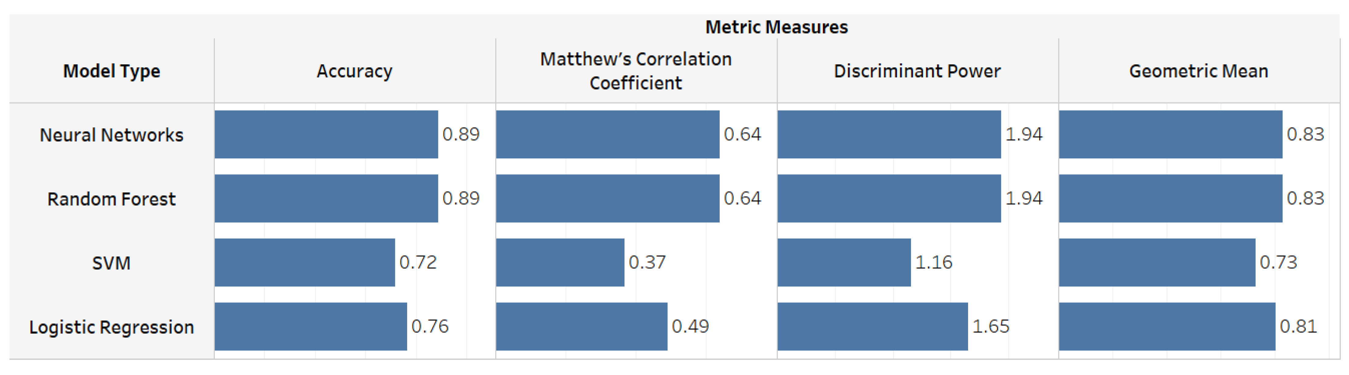
| Accuracy | Neural Networks | 0.89 | 0.79 | 0.78 | 0.81 | 0.82 | 0.84 |
| Random Forest | 0.89 | 0.69 | 0.73 | 0.75 | 0.87 | 0.83 | |
| Discriminant Power | Neural Networks | 1.94 | 0.95 | 0.82 | 0.90 | 1.87 | 1.33 |
| Random Forest | 1.94 | 0.64 | 0.29 | 0.71 | 2.09 | 1.19 | |
| Geometric Mean | Neural Networks | 0.83 | 0.65 | 0.61 | 0.54 | 0.84 | 0.84 |
| Random Forest | 0.83 | 0.63 | 0.46 | 0.60 | 0.87 | 0.63 | |
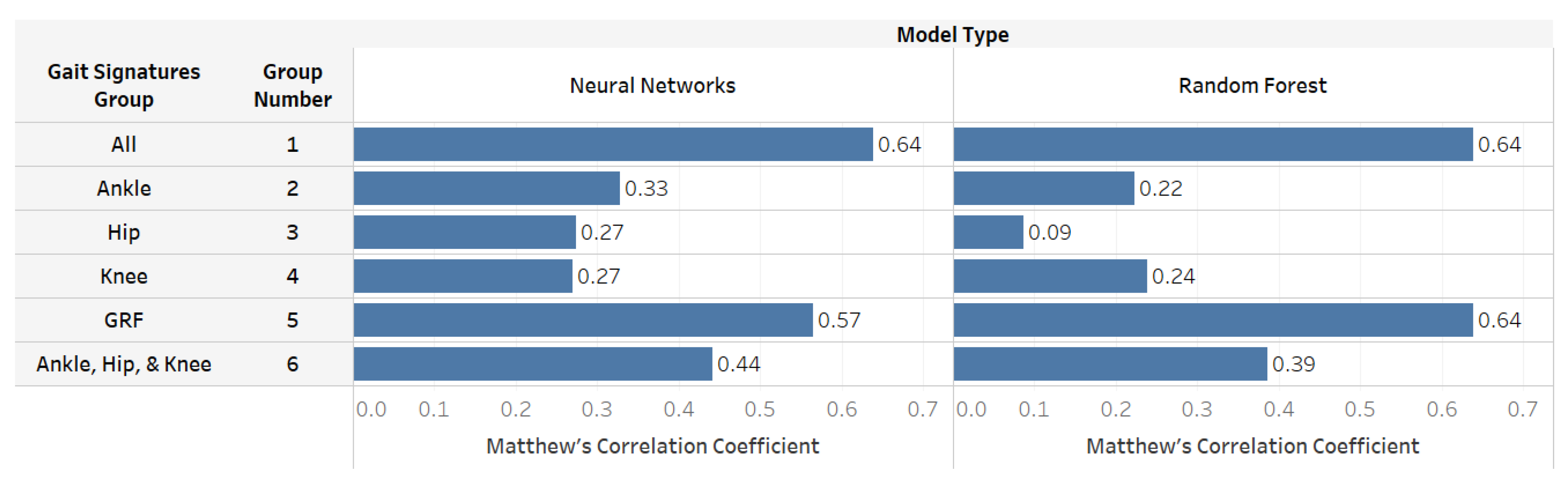
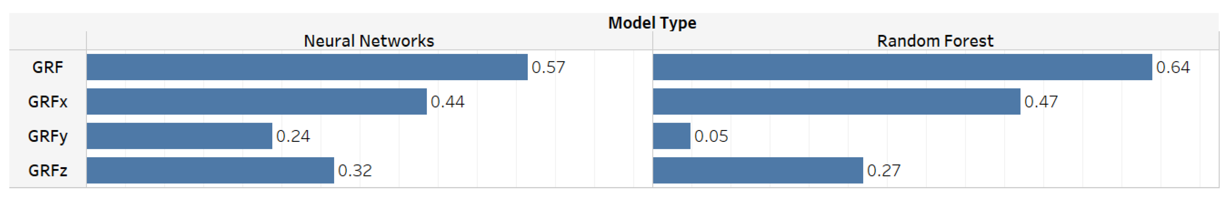
| Matthew’s Correlation Coefficient | Neural Networks | 0.64 | 0.33 | 0.27 | 0.27 | 0.57 | 0.44 |
| Random Forest | 0.64 | 0.22 | 0.09 | 0.24 | 0.64 | 0.39 | |
| Best model type | Neural Networks, Random Forest | Neural Networks | Neural Networks | Neural Networks | Random Forest | Neural Networks | |
ML Performance Metrics Description:
| |||||||
Publisher’s Note: MDPI stays neutral with regard to jurisdictional claims in published maps and institutional affiliations. |
© 2022 by the authors. Licensee MDPI, Basel, Switzerland. This article is an open access article distributed under the terms and conditions of the Creative Commons Attribution (CC BY) license (https://creativecommons.org/licenses/by/4.0/).
Share and Cite
Al-Ramini, A.; Hassan, M.; Fallahtafti, F.; Takallou, M.A.; Rahman, H.; Qolomany, B.; Pipinos, I.I.; Alsaleem, F.; Myers, S.A. Machine Learning-Based Peripheral Artery Disease Identification Using Laboratory-Based Gait Data. Sensors 2022, 22, 7432. https://doi.org/10.3390/s22197432
Al-Ramini A, Hassan M, Fallahtafti F, Takallou MA, Rahman H, Qolomany B, Pipinos II, Alsaleem F, Myers SA. Machine Learning-Based Peripheral Artery Disease Identification Using Laboratory-Based Gait Data. Sensors. 2022; 22(19):7432. https://doi.org/10.3390/s22197432
Chicago/Turabian StyleAl-Ramini, Ali, Mahdi Hassan, Farahnaz Fallahtafti, Mohammad Ali Takallou, Hafizur Rahman, Basheer Qolomany, Iraklis I. Pipinos, Fadi Alsaleem, and Sara A. Myers. 2022. "Machine Learning-Based Peripheral Artery Disease Identification Using Laboratory-Based Gait Data" Sensors 22, no. 19: 7432. https://doi.org/10.3390/s22197432
APA StyleAl-Ramini, A., Hassan, M., Fallahtafti, F., Takallou, M. A., Rahman, H., Qolomany, B., Pipinos, I. I., Alsaleem, F., & Myers, S. A. (2022). Machine Learning-Based Peripheral Artery Disease Identification Using Laboratory-Based Gait Data. Sensors, 22(19), 7432. https://doi.org/10.3390/s22197432