
Qualitative Classification of Lubricating Oil Wear Particle Morphology Based on Coaxial Capacitive Sensing Network and SVM


Abstract
:1. Introduction
2. Qualitative Classification Principle of Wear Particle Morphology Based on Coaxial Capacitive Sensor Network
2.1. Working Principle of Coaxial Capacitance Sensor Network
2.2. Qualitative Classification Method of Wear Particle Morphology
3. Overview of Support Vector Machine and Model Optimization Algorithm
3.1. Support Vector Machine
3.2. K-Means
- (a)
- Select samples from the initialized data set as the original cluster center;
- (b)
- The Euclidean distance from to K cluster centers of each sample is calculated respectively, and each sample is classified into the category corresponding to the cluster center with the smallest distance by using the nearest neighbor principle;
- (c)
- For each class , recalculate the cluster center of the class (i.e., the centroid of all samples of the class);
- (d)
- Repeat steps (b) and (c) until the new cluster center remains unchanged.
3.3. GridSearchCV
3.4. Parametric Analysis of Capacitive Sensor Network
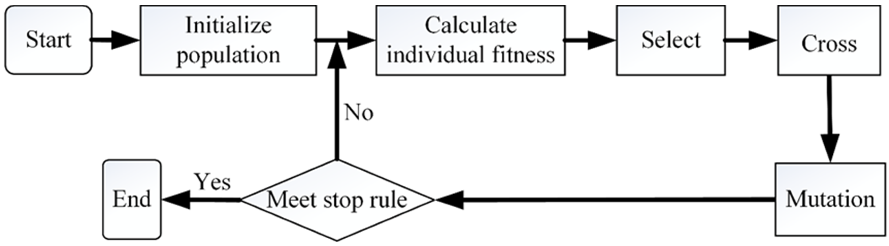
3.5. Genetic Algorithm
4. Construction and Verification of Qualitative Classification Model of Wear Particles
4.1. Construction of Qualitative Classification Model Based on Simulation of Wear Particles with Different Forms
4.1.1. Data Sampling and Labeling
4.1.2. Data Preprocessing Based on K-MEANS Algorithm
- (e)
- The data are classified according to the wear type. Each category is a separate data set, and each data set only has one cluster center;
- (f)
- The clustering centers of different data sets are calculated based on K-means algorithm;
- (g)
- Set the threshold to eliminate the samples far away from the cluster center.
4.1.3. Selection of Classification Model Parameters by Support Vector Machine
5. Performance Verification of Qualitative Classification Model Based on Experimental Wear Particles
5.1. Experiment Setup
5.2. Dividing Data and Labels
5.3. Selection of Classification Model Parameters Based on Support Vector Machine
6. Conclusions
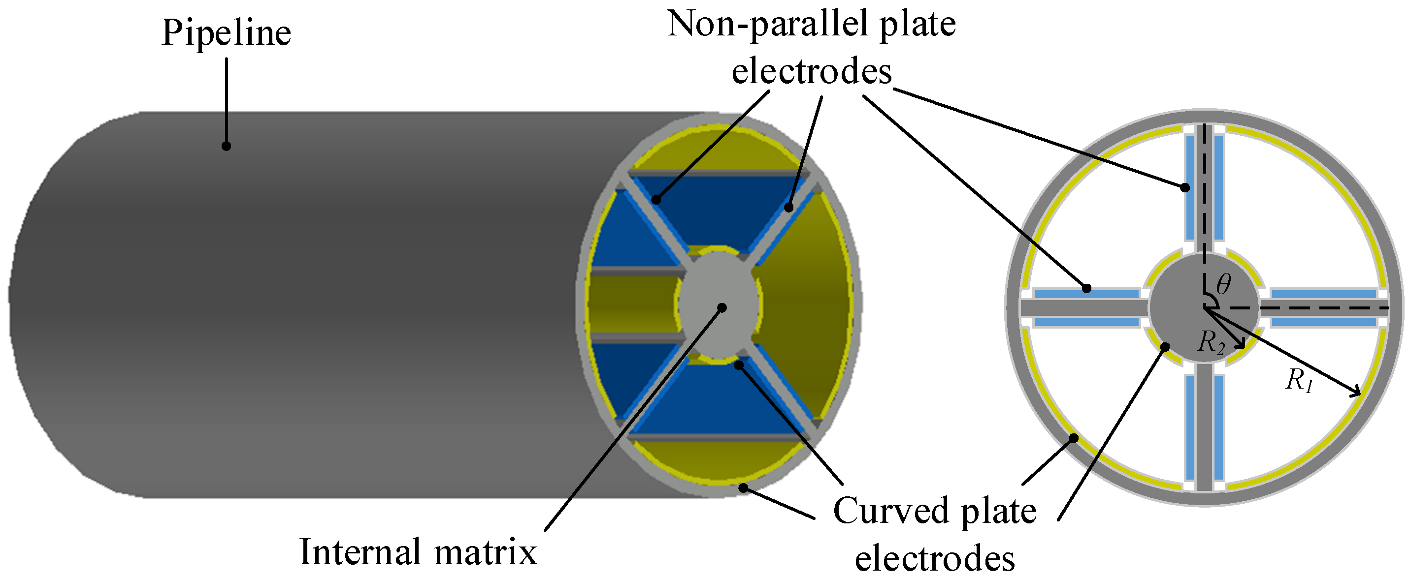
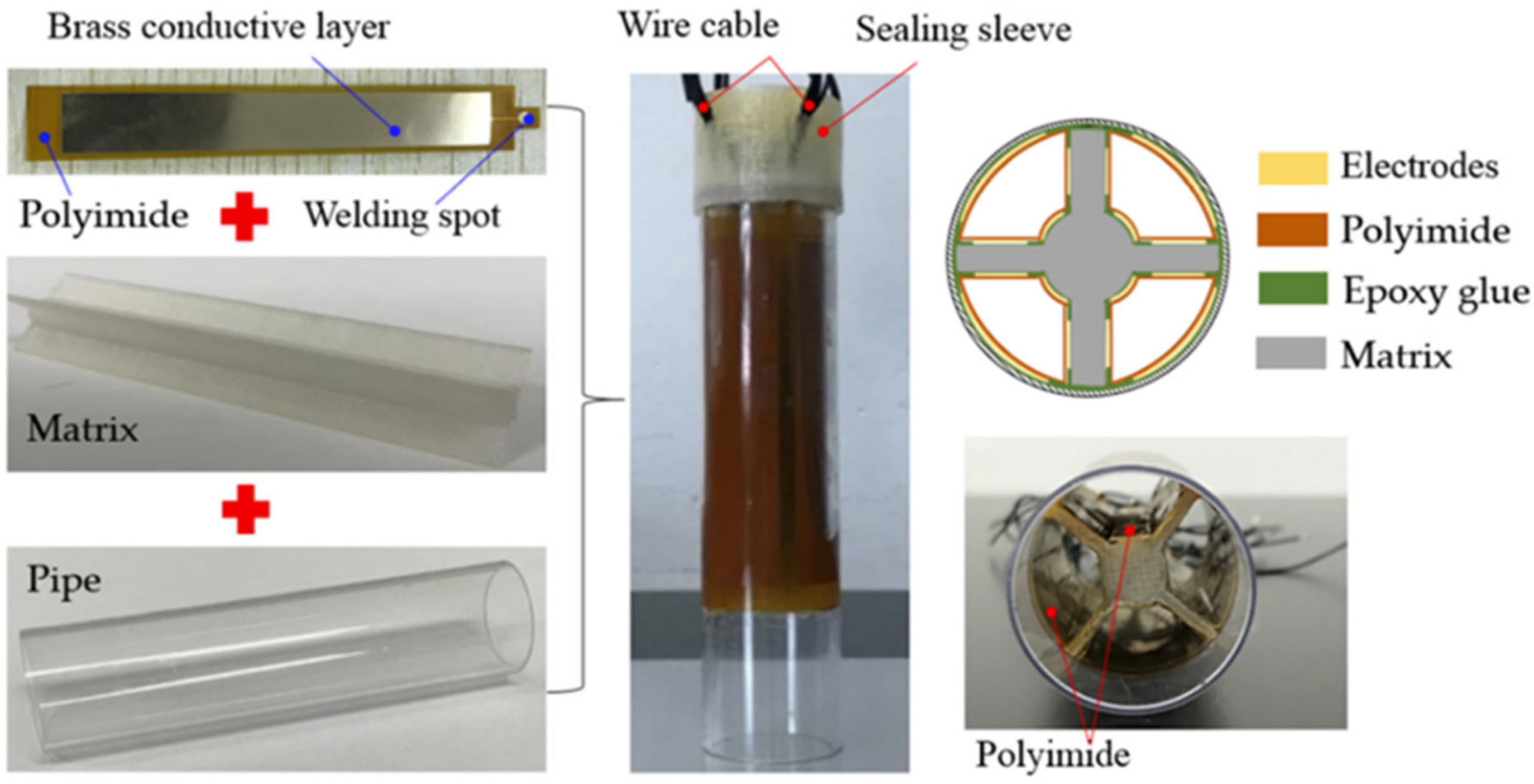
- The designed multi-group electrode plates can effectively monitor the wear particles on a micro scale. Coaxial capacitive sensor network can obtain multi-dimensional information characterizing wear particles.
- The optimized SVM can accurately classify the shape of lubricating oil wear particles. The classification accuracy of simulation data is 96.35%, and that of experimental data is 95.24%.
- The coaxial capacitance sensor network and support vector machine can be used to qualitatively classify the morphology of lubricating oil wear particles.
Author Contributions
Funding
Institutional Review Board Statement
Informed Consent Statement
Data Availability Statement
Acknowledgments
Conflicts of Interest
References
- Wakiru, J.M.; Pintelon, L.; Muchiri, P.N.; Chemweno, P.K. A review on lubricant condition monitoring information analysis for maintenance decision support. Mech. Syst. Signal Process. 2018, 118, 108–132. [Google Scholar] [CrossRef]
- Gao, T.; Han, Z.; Wu, D.; Li, Y.; Wang, Y. In situ collection and analysis of oil debris based on multi-physical field synthesis effect. J. Chin. Inst. Eng. 2020, 43, 339–345. [Google Scholar] [CrossRef]
- Guan, L.; Feng, X.; Xiong, G.; Xie, J. Application of dielectric spectroscopy for engine lubricating oil degradation monitoring. Sens. Actuators A Phys. 2011, 168, 22–29. [Google Scholar] [CrossRef]
- Matsumoto, K.; Tokunaga, T.; Kawabata, M. Engine Seizure Monitoring System Using Wear Debris Analysis and Particle Measurement. SAE Tech. Pap. 2016, 1, 5. [Google Scholar]
- Wang, S.; Wu, T.; Wang, K. Automated 3D ferrograph image analysis for similar particle identification with the knowledge-embedded double-CNN model. Wear 2021, 476, 203696. [Google Scholar] [CrossRef]
- Wang, S.; Wu, T.H.; Shao, T.; Peng, Z.X. Integrated model of BP neural network and CNN algorithm for automatic wear debris classification. Wear 2019, 426–427, 1761–1770. [Google Scholar] [CrossRef]
- Wang, S.; Wu, T.; Zheng, P.; Kwok, N. Optimized CNN model for identifying similar 3D wear particles in few samples. Wear 2020, 460–461, 203477. [Google Scholar] [CrossRef]
- Peng, P.; Wang, J. Wear particle classification considering particle overlapping. Wear 2019, 422–423, 119–127. [Google Scholar] [CrossRef]
- Iwai, Y.; Honda, T.; Miyajima, T.; Yoshinaga, S.; Higashi, M.; Fuwa, Y.J.T.I. Quantitative estimation of wear amounts by real time measurement of wear debris in lubricating oil. Tribol. Int. 2010, 43, 388–394. [Google Scholar] [CrossRef]
- Xu, C.; Zhang, P.; Wang, H.; Li, Y.; Lv, C. Ultrasonic echo waveshape features extraction based on QPSO-matching pursuit for online wear debris discrimination. Mech. Syst. Signal Process. 2015, 60–61, 301–315. [Google Scholar] [CrossRef]
- Wu, Y.; Zhang, H.; Zeng, L.; Chen, H.; Sun, Y. Determination of metal particles in oil using a microfluidic chip-based inductive sensor. Instrum. Sci. Technol. 2016, 44, 259–269. [Google Scholar] [CrossRef]
- Hong, W.; Wang, S.; Tomovic, M.M.; Liu, H.; Wang, X. A new debris sensor based on dual excitation sources for online debris monitoring. Meas. Sci. Technol. 2015, 26, 095101. [Google Scholar] [CrossRef]
- Powrie, H. Use of electrostatic technology for aero engine oil system monitoring. In Proceedings of the 2000 IEEE Aerospace Conference, Big Sky, MT, USA, 25 March 2000; IEEE: Piscataway, NJ, USA, 2000; Volume 6, pp. 57–72. [Google Scholar]
- Du, L.; Zhu, X.; Han, Y.; Zhao, L.; Zhe, J. Improving sensitivity of an inductive pulse sensor for detection of metallic wear debris in lubricants using parallel LC resonance method. Meas. Sci. Technol. 2013, 24, 075106. [Google Scholar] [CrossRef]
- Du, L.; Zhe, J. On-line wear debris detection in lubricating oil for condition based health monitoring of rotary machinery. Recent Adv. Electr. Electron. Eng. 2011, 4, 1–9. [Google Scholar] [CrossRef]
- Han, Z.; Wang, Y.; Qing, X. Characteristics Study of In-Situ Capacitive Sensor for Monitoring Lubrication Oil Debris. Sensors 2017, 17, 2851. [Google Scholar] [CrossRef]
- Wang, Y.; Han, Z.; Gao, T.; Qing, X. In-situ capacitive sensor for monitoring debris of lubricant oil. Ind. Lubr. Tribol. 2018, 70, 1310–1319. [Google Scholar] [CrossRef]
- Bowen, E.R.; Westcott, V.C. Wear Particle Atlas; Maritime Technical Information Facility: Lakehurst, NJ, USA, 1976. [Google Scholar]
- Anderson, D.P. Wear Particle Atlas. (Revised); Foxboro Analytical: Burlington, MA, USA, 1982. [Google Scholar]
- Wang, Y.; Lin, T.; Wu, D.; Zhu, L.; Qing, X.; Xue, W. A New In Situ Coaxial Capacitive Sensor Network for Debris Monitoring of Lubricating Oil. Sensors 2022, 22, 1777. [Google Scholar] [CrossRef]
- An, Z.; Wang, X.; Li, B.; Xiang, Z.; Zhang, B. Robust visual tracking for UAVs with dynamic feature weight selection. Appl. Intell. 2022, 52, 1–14. [Google Scholar] [CrossRef]
- Chen, H.; Miao, F.; Chen, Y.; Xiong, Y.; Chen, T. A hyperspectral image classification method using multifeature vectors and optimized KELM. IEEE J. Sel. Top. Appl. Earth Obs. Remote Sens. 2021, 14, 2781–2795. [Google Scholar] [CrossRef]
- Keller, J.M.; Gray, M.R.; Givens, J.A. A fuzzy k-nearest neighbor algorithm. IEEE Trans. Syst. Man Cybern. 1985, 4, 580–585. [Google Scholar] [CrossRef]
- Wold, S.; Esbensen, K.; Geladi, P. Principal component analysis. Chemom. Intell. Lab. Syst. 1987, 2, 37–52. [Google Scholar] [CrossRef]
- Hartigan, J.A.; Wong, M.A. Algorithm AS 136: A k-means clustering algorithm. J. R. Stat. Soc. Ser. C 1979, 28, 100–108. [Google Scholar] [CrossRef]
- Ranjan, G.S.K.; Verma, A.K.; Radhika, S. K-nearest neighbors and grid search cv based real time fault monitoring system for industries. In Proceedings of the 2019 IEEE 5th International Conference for Convergence in Technology (I2CT), Pune, India, 29–31 March 2019; IEEE: Piscataway, NJ, USA, 2019; pp. 1–5. [Google Scholar]
- Eberhart, R.; Kennedy, J. A new optimizer using particle swarm theory. In Proceedings of the MHS’95 Proceedings of the Sixth International Symposium on Micro Machine and Human Science, Nagoya, Japan, 4–6 October 1995; IEEE Service Center: Piscataway, NJ, USA, 1995; pp. 39–43. [Google Scholar]
- Zhou, X.; Ma, H.; Gu, J.; Chen, H.; Deng, W. Parameter adaptation-based ant colony optimization with dynamic hybrid mechanism. Eng. Appl. Artif. Intell. 2022, 114, 105139. [Google Scholar] [CrossRef]
- Wu, D.; Wu, C. Research on the Time-Dependent Split Delivery Green Vehicle Routing Problem for Fresh Agricultural Products with Multiple Time Windows. Agriculture 2022, 12, 793. [Google Scholar] [CrossRef]
- Holland, J.H. Adaptation in Natural and Artificial Systems: An Introductory Analysis with Applications to Biology, Control, and Artificial Intelligence; MIT Press: Cambridge, MA, USA, 1992. [Google Scholar]


| Wear Type | Wear Characteristics | |||
|---|---|---|---|---|
| Equivalent Diameter (µm) | Thickness (µm) | Slenderness Ratio | Form | |
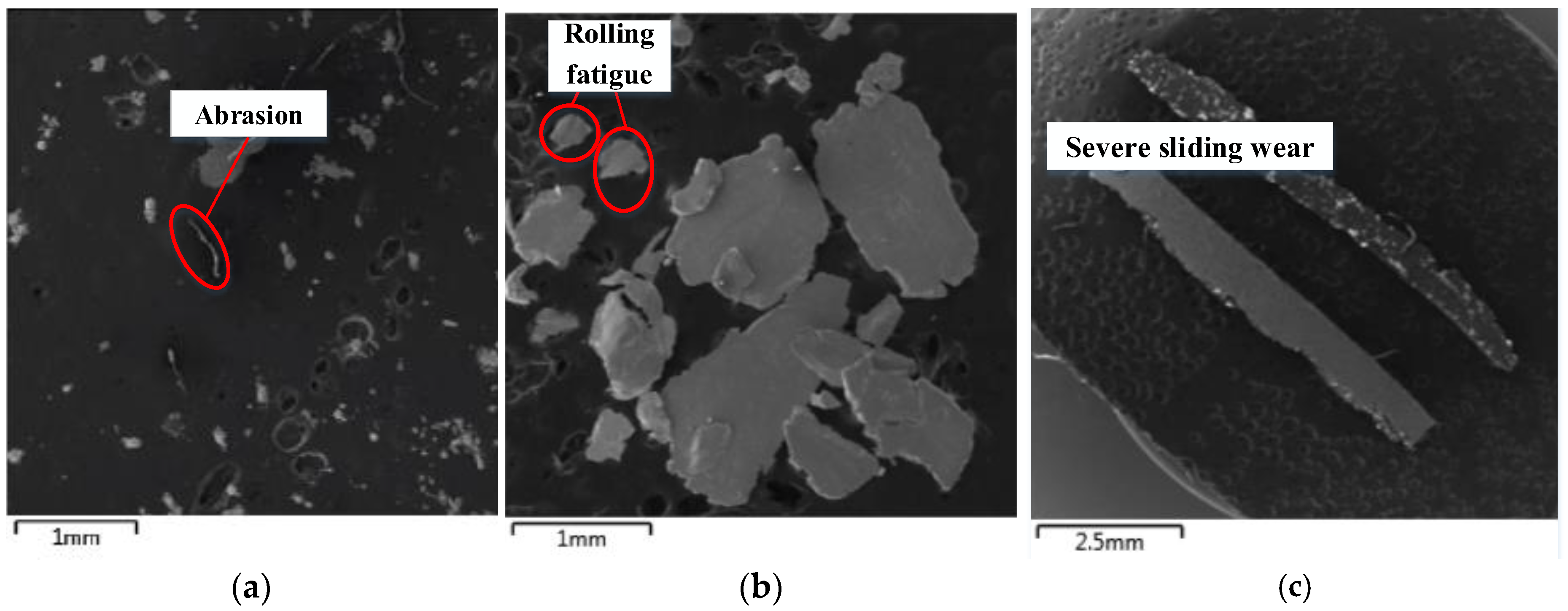
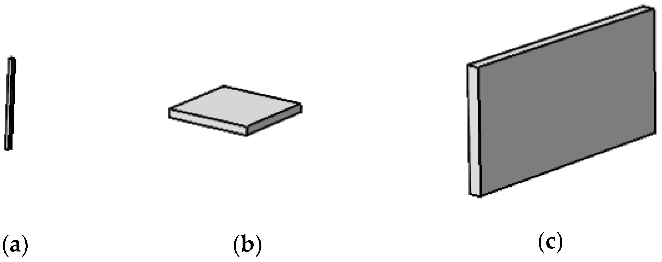
| Rubbing | 0.5–15 | 0.15–1 | 3:1–10:1 | Minimal shape |
| Cutting | 25–100 (length) | 2–5 (width) | 12:1–20:1 | Slender type |
| Rolling contact fatigue | 10–100 | 1–10 | 10:1 | Block/flat |
| Sliding and rolling fatigue | NA | NA | 4:1–10:1 | Irregular shape |
| Severe sliding wear | >15 | NA | 10:1 | Striped |
| Kernel Function | Expression | Advantage | Shortcoming |
|---|---|---|---|
| Linear | Simple and strong interpretability. | It can only solve the linear separable problem. | |
| RBF | It can be mapped to wireless dimension with only one parameter. | Poor interpretability, slow calculation speed, and easy over fitting. | |
| Poly | It can solve nonlinear problems. | There are many parameters, so it is not suitable for idempotents of large order of magnitude. |
| Wear Type (Label) | Wear Characteristics | ||
|---|---|---|---|
| Equivalent Diameter (µm) | Thickness (µm) | Slenderness Ratio | |
| cutting | 25–100 | 2–5 | 12:1–20:1 |
| rolling | 10–100 | 1–10 | 10:1 |
| sliding | >15 | 10:1 | |
| Wear Type | Geometric Parameter | Parameter Range (µm) | Parameter Step (µm) | Number of Simulation Groups |
|---|---|---|---|---|
| Abrasion | Width | 25~100 | 5 | 256 |
| Depth | 2~5 | 1 | ||
| Height | 2~5 | 1 | ||
| Rolling fatigue | Width | 10~100 | 10 | 1000 |
| Depth | 1~10 | 1 | ||
| Height | 1~10 | 1 | ||
| Severe sliding wear | Width | 30~100 | 5 | 120 |
| Depth | One tenth of the width | NA | ||
| Height | 30~100 | 5 |
| Name | Value | Describe |
|---|---|---|
| ε0 | 8.854187817 × 10⁻¹² F/m | Vacuum Dielectric Constant |
| ε | Variable | Dielectric relative permittivity |
| l | 80 mm | Sensor network length |
| R1 | Parameters to be determined | Inner core radius |
| R2 | 11 mm | Sensor network radius |
| Method | Determined Parameters | Training Set Accuracy | Test Set Accuracy |
|---|---|---|---|
| GridSearchCV | C = 1.5 G = 5.4 | 93.90% | 94.52% |
| PSO | C = 7.10 G = 3.59 | 94.21% | 95.43% |
| GA | C = 7.65 G = 7.67 | 95.43% | 96.35% |
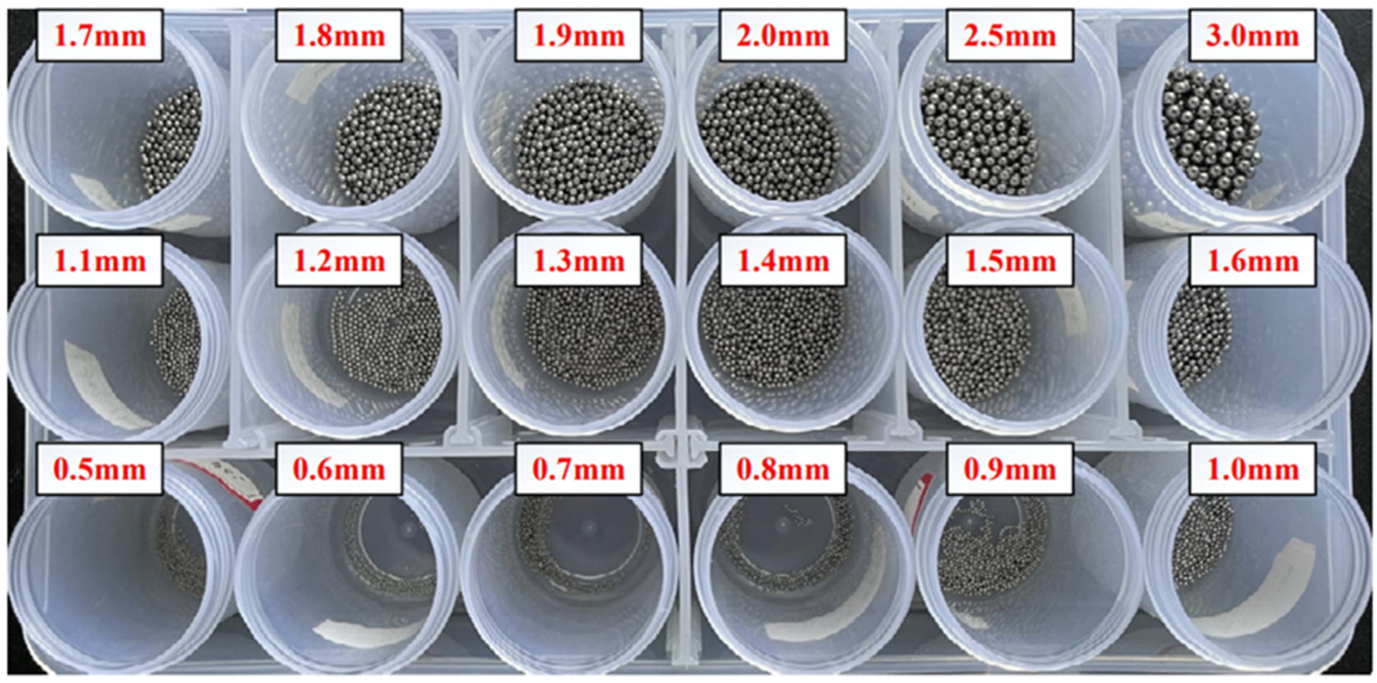
| Size (mm) | Type |
|---|---|
| 3.0, 2.5 | big |
| 2.0, 1.9, 1.8, 1.7, 1.6, 1.5, 1.4, 1.3, 1.2, 1.1 | medium |
| 1.0, 0.9, 0.8, 0.7, 0.6, 0.5 | small |
| Method | Determined Parameters | Training Set Accuracy | Test Set Accuracy |
|---|---|---|---|
| GridSearchCV | C = 0.9 G = 8.70 | 88.71% | 95.24% |
| PSO | C= 8.45 G = 4.55 | 95.16% | 95.24% |
| GA | C= 7.24 G = 3.96 | 90.32% | 95.24% |
| Oil Wear Particle Monitoring Sensors | Wear Particle Count | Wear Particle Morphology Recognition |
|---|---|---|
| Capacitance Kurt counter | Realizable | Not achievable |
| Microchannel capacitance sensor | Realizable | Not achievable |
| Coaxial Capacitive Sensing Network and SVM | Realizable | Realizable |
Publisher’s Note: MDPI stays neutral with regard to jurisdictional claims in published maps and institutional affiliations. |
© 2022 by the authors. Licensee MDPI, Basel, Switzerland. This article is an open access article distributed under the terms and conditions of the Creative Commons Attribution (CC BY) license (https://creativecommons.org/licenses/by/4.0/).
Share and Cite
Zhu, L.; Xiao, X.; Wu, D.; Wang, Y.; Qing, X.; Xue, W. Qualitative Classification of Lubricating Oil Wear Particle Morphology Based on Coaxial Capacitive Sensing Network and SVM. Sensors 2022, 22, 6653. https://doi.org/10.3390/s22176653
Zhu L, Xiao X, Wu D, Wang Y, Qing X, Xue W. Qualitative Classification of Lubricating Oil Wear Particle Morphology Based on Coaxial Capacitive Sensing Network and SVM. Sensors. 2022; 22(17):6653. https://doi.org/10.3390/s22176653
Chicago/Turabian StyleZhu, Ling, Xiangwen Xiao, Diheng Wu, Yishou Wang, Xinlin Qing, and Wendong Xue. 2022. "Qualitative Classification of Lubricating Oil Wear Particle Morphology Based on Coaxial Capacitive Sensing Network and SVM" Sensors 22, no. 17: 6653. https://doi.org/10.3390/s22176653
APA StyleZhu, L., Xiao, X., Wu, D., Wang, Y., Qing, X., & Xue, W. (2022). Qualitative Classification of Lubricating Oil Wear Particle Morphology Based on Coaxial Capacitive Sensing Network and SVM. Sensors, 22(17), 6653. https://doi.org/10.3390/s22176653