XGBLoc: XGBoost-Based Indoor Localization in Multi-Building Multi-Floor Environments


Abstract
:1. Introduction
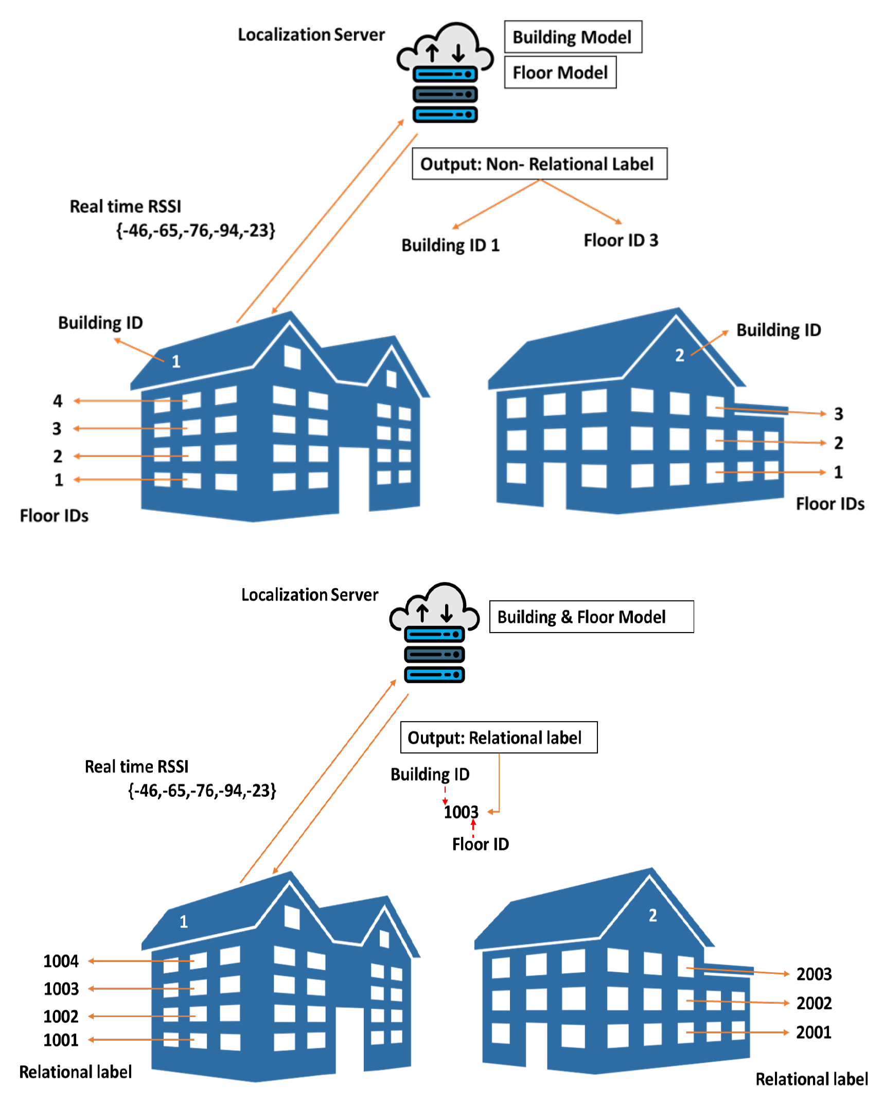
- Create a novel and uniquely-combined synthetic label (also called relational label) directly associating a building ID with a floor ID in a multi-building multi-floor environment. Using this relational labeling (RL) rather than existing non-relational labeling (NRL; or independent labeling, where building ID and floor ID are separately dealt with), the presented ML-based classification model predicts target locations in such complex hierarchical environments accurately and consistently.
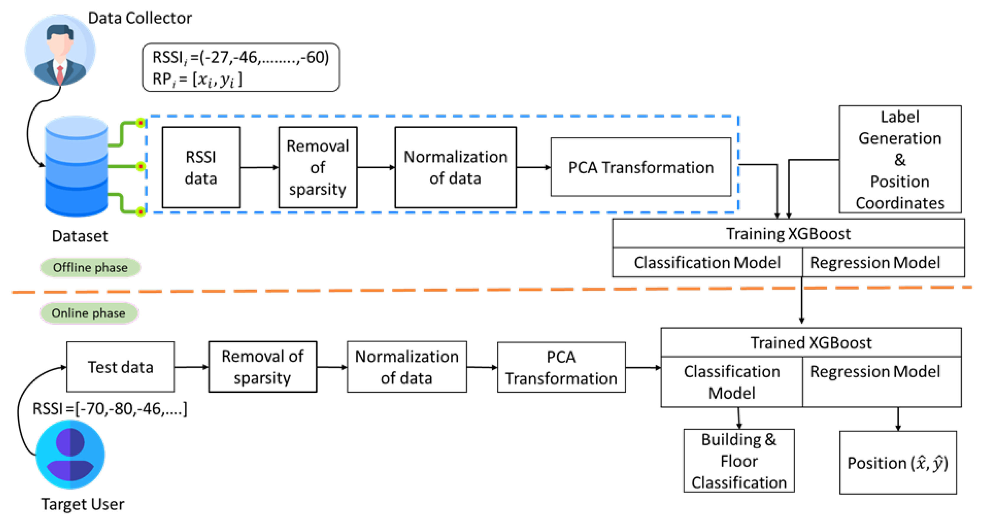
- Propose an XGBoost-based IL method using RL, termed as XGBLoc, that improves localization accuracy in the multi-building multi-floor environments. XGBLoc is especially good for the classification and regression over such hierarchical and complex indoor environments. XGBLoc employs PCA both for dimensionality reduction and input dataset (i.e, RSSI fingerprints) denoising. After PCA transformation, XGBLoc is trained and tested to predict target location with an improved accuracy over dynamic (mobile) indoor channel conditions including multipath fading.
- Evaluate XGBLoc over the following three publicly available datasets: UJIIndoorLoc [18], Tampere [19], and Alcala [20]. Simulation results validate that the proposed scheme has a superior localization performance over existing ML/DL schemes (see Section 4 for the details) especially at the perspective of localization accuracy as well as system complexity.
2. Related Works
Shortcomings of Existing Schemes
3. Proposed Methodology
3.1. Proposed System Architecture
3.2. Input and Output Specification
3.3. Objective Function of Proposed XGBoost-Based ML Model
- With a similarity score, XGBoost prunes the tree. It calculates the node’s gain as the difference between the node’s similarity and the children’s similarity score. When the node’s gain is found to be nominal, it simply stops constructing the tree to a greater extent.
- In real-world applications, classification performance, computational cost, and hyperparameter optimization are critical factors of choosing a good classifier. In the paper, we choose XGBoost as such a good candidate for the IL applications where a target object is localized over a multi-building multi-floor environment. Moreover, when compared to traditional ML/DL classifiers, XGBoost is capable of handling real-time data with many variations.
- Especially, we use relational labels representing that hierarchical environment in a given dataset and train XGBoost using such translated tabular data. The proposed algorithm, simply termed as XGBLoc, performs better on those tabular data even with fewer data samples, when compared to other ML/DL algorithms.
- Furthermore, to deal with over- and under-fitting, those existing ML/DL algorithms require extensive hyperparameter tuning. For instance, ML algorithms such as RF, KNN, and so forth require longer computational time. Furthermore, DL algorithms require a large number of data samples to perform well. However, XGBLoc requests a relatively simple hyperparameter tuning.
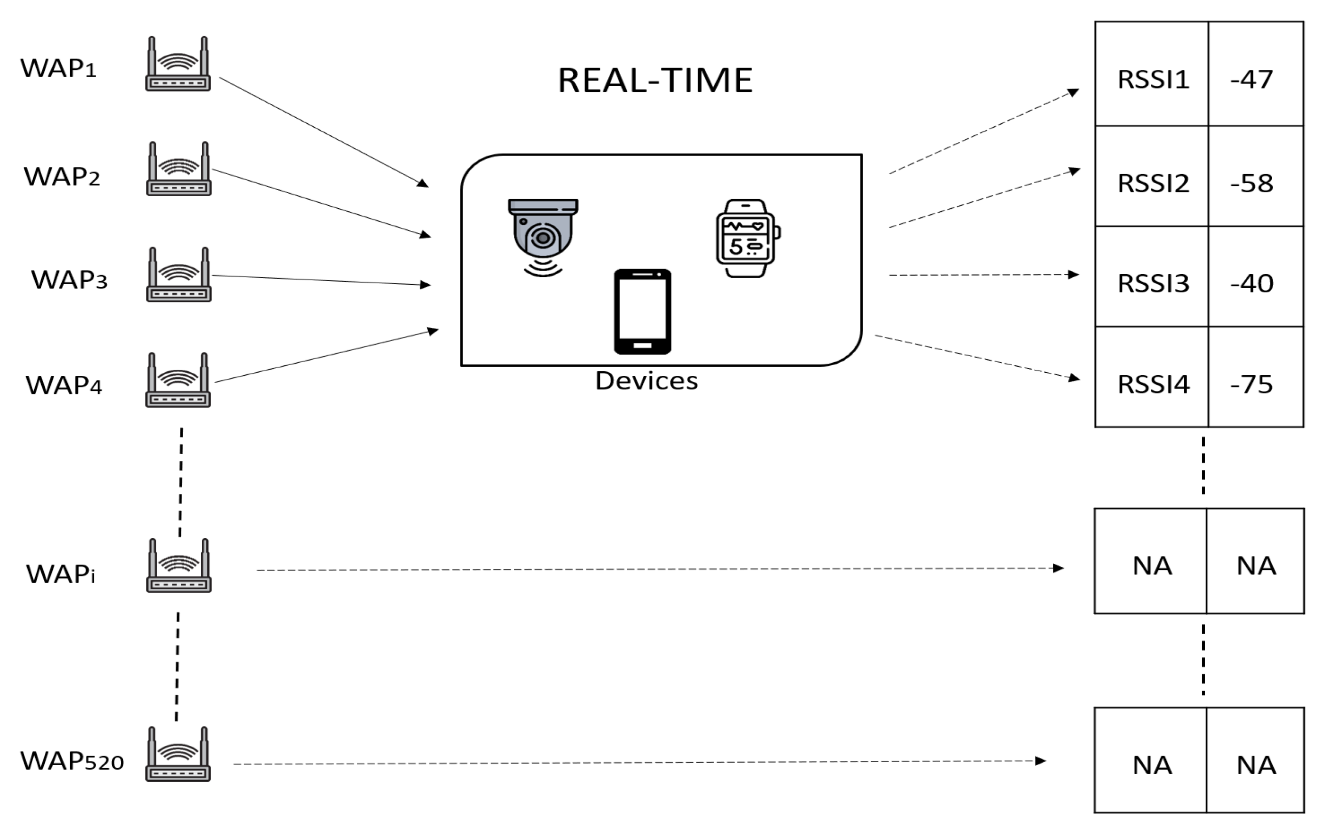
3.4. RSSI Data and Preprocessing
| Algorithm 1 Pseudo code of proposed XGBLoc scheme |
|
4. Performance Analysis
4.1. Results on Benchmark UJIIndoor Dataset
4.1.1. Effect of Explained Variance Ratio on Performance
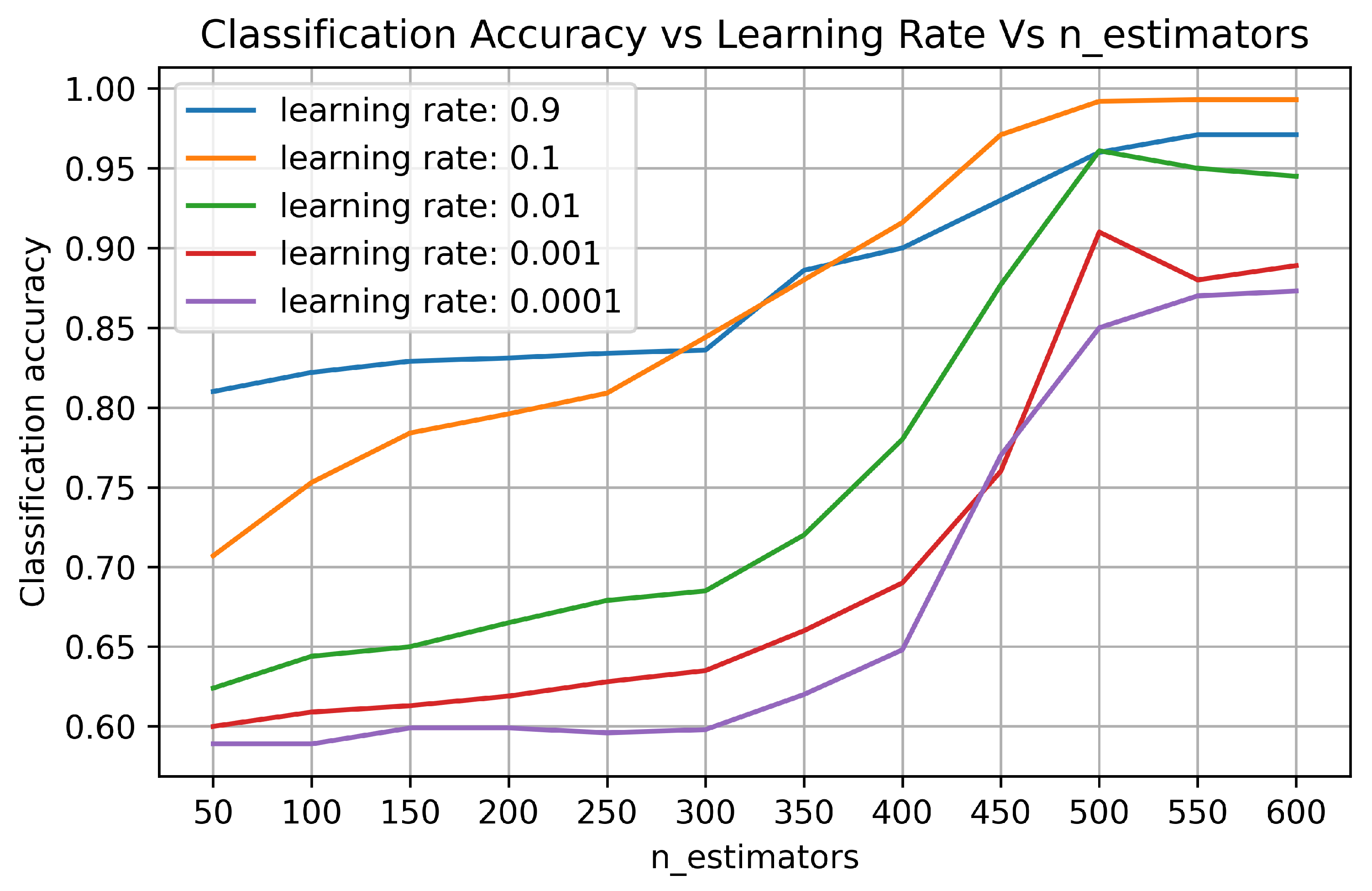
4.1.2. Effect of Hyperparameter Tuning on Performance
4.1.3. Localization Performance Comparison
4.2. Results on Additional Datasets
4.2.1. Results on Tampere Dataset
4.2.2. Results on Alcala Dataset
5. Conclusions
Author Contributions
Funding
Institutional Review Board Statement
Informed Consent Statement
Data Availability Statement
Conflicts of Interest
References
- Obeidat, H.; Shuaieb, W.; Obeidat, O.; Abd-Alhameed, R. A review of indoor localization techniques and wireless technologies. Wirel. Pers. Commun. 2021, 119, 289–327. [Google Scholar] [CrossRef]
- He, S.; Chan, S.H.G. Wi-Fi fingerprint-based indoor positioning: Recent advances and comparisons. IEEE Commun. Surv. Tutor. 2015, 18, 466–490. [Google Scholar] [CrossRef]
- Zhao, F.; Huang, T.; Wang, D. A probabilistic approach for WiFi fingerprint localization in severely dynamic indoor environments. IEEE Access 2019, 7, 116348–116357. [Google Scholar] [CrossRef]
- Zafari, F.; Gkelias, A.; Leung, K.K. A survey of indoor localization systems and technologies. IEEE Commun. Surv. Tutor. 2019, 21, 2568–2599. [Google Scholar] [CrossRef]
- Niu, J.; Wang, B.; Cheng, L.; Rodrigues, J.J.P.C. WicLoc: An Indoor Localization System Based on WiFi Fingerprints and Crowdsourcing. In Proceedings of the 2015 IEEE International Conference on Communications (ICC), London, UK, 8–12 June 2015; pp. 3008–3013. [Google Scholar]
- Keskin, M.F.; Sezer, A.D.; Gezici, S. Localization via visible light systems. Proc. IEEE 2018, 106, 1063–1088. [Google Scholar] [CrossRef]
- Zhang, C.; Zhang, X. Visible light localization using conventional light fixtures and smartphones. IEEE Trans. Mob. Comput. 2019, 18, 2968–2983. [Google Scholar] [CrossRef]
- Liu, R.; Yuen, C.; Do, T.N.; Tan, U.X. Fusing similarity-based sequence and dead reckoning for indoor positioning without training. IEEE Sens. J. 2017, 17, 4197–4207. [Google Scholar] [CrossRef]
- Soltanaghaei, E.; Kalyanaraman, A.; Whitehouse, K. Multipath Triangulation: Decimeter-Level WiFi Localization and Orientation with a Single Unaided Receiver. In Proceedings of the 16th Annual International Conference on Mobile Systems, Applications, and Services, Munich, Germany, 10–15 June 2018; pp. 376–388. [Google Scholar]
- Yassin, A.; Nasser, Y.; Awad, M.; Al-Dubai, A.; Liu, R.; Yuen, C.; Raulefs, R.; Aboutanios, E. Recent advances in indoor localization: A survey on theoretical approaches and applications. IEEE Commun. Surv. Tutor. 2016, 19, 1327–1346. [Google Scholar] [CrossRef]
- Zhu, X.; Qu, W.; Qiu, T.; Zhao, L.; Atiquzzaman, M.; Wu, D.O. Indoor intelligent fingerprint-based localization: Principles, approaches and challenges. IEEE Commun. Surv. Tutor. 2020, 22, 2634–2657. [Google Scholar] [CrossRef]
- Singh, N.; Choe, S.; Punmiya, R. Machine learning based indoor localization using Wi-Fi RSSI fingerprints: An overview. IEEE Access 2021, 9, 127150–127174. [Google Scholar] [CrossRef]
- Song, X.; Fan, X.; Xiang, C.; Ye, Q.; Liu, L.; Wang, Z.; He, X.; Yang, N.; Fang, G. A novel convolutional neural network based indoor localization framework with WiFi fingerprinting. IEEE Access 2019, 7, 110698–110709. [Google Scholar] [CrossRef]
- Chen, T.; Guestrin, C. XGBoost: A Scalable Tree Boosting System. In Proceedings of the 22nd ACM SIGKDD International Conference on Knowledge Discovery and Data Mining, San Francisco, CA, USA, 13–17 August 2016; pp. 785–794. [Google Scholar]
- Punmiya, R.; Choe, S. Energy theft detection using gradient boosting theft detector with feature engineering-based preprocessing. IEEE Trans. Smart Grid 2019, 10, 2326–2329. [Google Scholar] [CrossRef]
- Ringnér, M. What is principal component analysis? Nat. Biotechnol. 2008, 26, 303–304. [Google Scholar] [CrossRef]
- Wall, M.E.; Rechtsteiner, A.; Rocha, L.M. Singular Value Decomposition and Principal Component Analysis. In A Practical Approach to Microarray Data Analysis; Springer: Berlin/Heidelberg, Germany, 2003; pp. 91–109. [Google Scholar]
- Torres-Sospedra, J.; Montoliu, R.; Martínez-Usó, A.; Avariento, J.P.; Arnau, T.J.; Benedito-Bordonau, M.; Huerta, J. UJIIndoorLoc: A New Multi-Building and Multi-Floor Database for WLAN Fingerprint-Based Indoor Localization Problems. In Proceedings of the 2014 IEEE International Conference on Indoor Positioning and Indoor Navigation (IPIN), Busan, Korea, 27–30 October 2014; pp. 261–270. [Google Scholar]
- Lohan, E.S.; Torres-Sospedra, J.; Leppäkoski, H.; Richter, P.; Peng, Z.; Huerta, J. Wi-Fi crowdsourced fingerprinting dataset for indoor positioning. Data 2017, 2, 32. [Google Scholar] [CrossRef]
- Montoliu, R.; Sansano, E.; Torres-Sospedra, J.; Belmonte, O. IndoorLoc Platform: A Public Repository for Comparing and Evaluating Indoor Positioning Systems. In Proceedings of the 2017 International Conference on Indoor Positioning and Indoor Navigation (IPIN), Sapporo, Japan, 18–21 September 2017. [Google Scholar]
- Ge, X.; Qu, Z. Optimization WiFi Indoor Positioning KNN Algorithm Location-Based Fingerprint. In Proceedings of the 7th IEEE International Conference on Software Engineering and Service Science (ICSESS), Beijing, China, 26–28 August 2016; pp. 135–137. [Google Scholar]
- Hu, J.; Liu, D.; Yan, Z.; Liu, H. Experimental analysis on weight K-nearest neighbor indoor fingerprint positioning. IEEE Internet Things J. 2018, 6, 891–897. [Google Scholar] [CrossRef]
- Zhang, S.; Guo, J.; Wang, W.; Hu, J. Indoor 2.5 D positioning of WiFi based on SVM. In Proceedings of the 2018 IEEE Ubiquitous Positioning, Indoor Navigation and Location-Based Services (UPINLBS), Wuhan, China, 22–23 March 2018; pp. 1–7. [Google Scholar]
- Seçkin, A.Ç.; Coşkun, A. Hierarchical fusion of machine learning algorithms in indoor positioning and localization. Appl. Sci. 2019, 9, 3665. [Google Scholar] [CrossRef]
- Tang, Z.; Li, S.; Kim, K.S.; Smith, J. Multi-output Gaussian process-based data augmentation for multi-building and multi-floor indoor localization. arXiv 2022, arXiv:2202.01980. [Google Scholar]
- Ahmed Elesawi, A.E.; Kim, K.S. Hierarchical Multi-Building And Multi-Floor Indoor Localization Based On Recurrent Neural Networks. In Proceedings of the 2021 9th International Symposium on Computing and Networking Workshops (CANDARW), Matsue, Japan, 21–24 November 2021; pp. 193–196. [Google Scholar]
- Laska, M.; Blankenbach, J. DeepLocBox: Reliable Fingerprinting-Based Indoor Area Localization. Sensors 2021, 21, 2000. [Google Scholar] [CrossRef] [PubMed]
- Jang, J.W.; Hong, S.N. Indoor Localization with WiFi Fingerprinting Using Convolutional Neural Network. In Proceedings of the 10th IEEE International Conference on Ubiquitous and Future Networks (ICUFN), Prague, Czech Republic, 3–6 July 2018; pp. 753–758. [Google Scholar]
- Laska, M.; Blankenbach, J. Multi-task neural network for position estimation in large-scale indoor environments. IEEE Access 2022, 10, 26024–26032. [Google Scholar] [CrossRef]
- Shwartz-Ziv, R.; Armon, A. Tabular data: Deep learning is not all you need. Inf. Fusion 2022, 81, 84–90. [Google Scholar] [CrossRef]
- Yu, T.; Zhu, H. Hyper-parameter optimization: A review of algorithms and applications. arXiv 2020, arXiv:2003.05689. [Google Scholar]
- Teorey, T.J.; Yang, D.; Fry, J.P. A logical design methodology for relational databases using the extended entity-relationship model. ACM Comput. Surv. (CSUR) 1986, 18, 197–222. [Google Scholar] [CrossRef] [Green Version]
- Bentéjac, C.; Csörgo, A.; Martínez-Muñoz, G. A comparative analysis of gradient boosting algorithms. Artif. Intell. Rev. 2021, 54, 1937–1967. [Google Scholar] [CrossRef]
- Yoo, J.; Park, J. Indoor localization based on Wi-Fi received signal strength indicators: Feature extraction, mobile fingerprinting, and trajectory learning. Appl. Sci. 2019, 9, 3930. [Google Scholar] [CrossRef]
- Qin, F.; Zuo, T.; Wang, X. CCpos: WiFi fingerprint indoor positioning system based on CDAE-CNN. Sensors 2021, 21, 1114. [Google Scholar] [CrossRef]
- Shlens, J. A tutorial on principal component analysis. arXiv 2014, arXiv:1404.1100. [Google Scholar]
- Jolliffe, I.T.; Cadima, J. Principal component analysis: A review and recent developments. Philos. Trans. R. Soc. A Math. Phys. Eng. Sci. 2016, 374, 20150202. [Google Scholar] [CrossRef]
- Berkvens, R.; Weyn, M.; Peremans, H. Localization Performance Quantification by Conditional Entropy. In Proceedings of the 2015 IEEE International Conference on Indoor Positioning and Indoor Navigation (IPIN), Banff, AB, Canada, 13–16 October 2015; pp. 1–7. [Google Scholar]
- Torres-Sospedra, J.; Montoliu, R.; Trilles, S.; Belmonte, Ó.; Huerta, J. Comprehensive analysis of distance and similarity measures for Wi-Fi fingerprinting indoor positioning systems. Expert Syst. Appl. 2015, 42, 9263–9278. [Google Scholar] [CrossRef]
- Nowicki, M.; Wietrzykowski, J. Low-Effort Place Recognition with WiFi Fingerprints Using Deep Learning. In Proceedings of the International Conference Automation; Springer: Berlin/Heidelberg, Germany, 2017; pp. 575–584. [Google Scholar]
- Kim, K.S.; Lee, S.; Huang, K. A scalable deep neural network architecture for multi-building and multi-floor indoor localization based on Wi-Fi fingerprinting. Big Data Anal. 2018, 3, 1–17. [Google Scholar] [CrossRef]
- Akram, B.A.; Akbar, A.H.; Shafiq, O. HybLoc: Hybrid indoor Wi-Fi localization using soft clustering-based random decision forest ensembles. IEEE Access 2018, 6, 38251–38272. [Google Scholar] [CrossRef]


| Ref. | P Dataset | Labels | Techniques Used | H Tuning | B/F Classification |
|---|---|---|---|---|---|
| [25] | ✓ | NRL | RNN | Extensive | ✓ |
| [26] | ✓ | NRL | RNN | Extensive | ✓ |
| [13] | ✓ | NRL | SAE, CNN | Extensive | ✓ |
| [27] | ✓ | NRL | DNN | Extensive | ✓ |
| [28] | ✓ | NRL | 2D Radio map, CNN | Extensive | ✓ |
| [29] | ✓ | NRL | m-CELL, 2D CNN | Extensive | ✓ |
| XGBLoc | ✓ | RL | PCA, XGBoost | Less | ✓ |
| Elements of Fingerprints () | Description |
|---|---|
| R | , and is RSSI value of ith access point. |
| Longitudinal values of location in meters. | |
| Latitudinal values of location in meters. | |
| Floor ID. | |
| Building ID. |
| Symbols | Description |
|---|---|
| D | Fingerprint dataset. |
| N | Total number of samples in dataset. |
| M | Total number of dimmensions/WAPs. |
| RSSI vector at ith RP. | |
| Position of ith RP. | |
| Coordinates of the . | |
| K | Total number of trees. |
| Predicted position of ith RP. | |
| Predicted coordinates of the . | |
| Loss function. | |
| Regularization term of the kth tree. |
| Hyperparameter | Value | Description |
|---|---|---|
| learning_rate or eta | 0.3 | Weighting factor for learning in gradient boosting. |
| gamma | 1 | Minimum loss reduction needed to render partition on a tree leaf node. |
| max_depth | 6 | Maximum depth of tree. |
| colsample_bytree | 1 | Subsample ratio of columns when constructing each tree. |
| lambda | 1 | L2 regularization term on weights. |
| loss function | multi:softprob reg:squarederror | Multiclass classification problem. Regression with squared loss. |
| n_estimators | 100 | Number of trees to be generated. |
| scale_pos_weight | 1 | Control the balance of positive and negative weights. |
| booster | gbtree | Use tree based model. |
| tree_method | gpu_hist | GPU implementation of faster histogram optimized approximate greedy algorithm. |
| Subsample | 1 | Subsample ratio of the training samples. |
| Explained Variance Ratio (EVR) | 0.7 | 0.8 | 0.9 |
|---|---|---|---|
| Classification Accuracy | 98% | 98.6% | 99.2% |
| 2-D Mean position error () | 5.2 m | 4.93 m | 5.01 m |
| Task | Hyperparameter | Output | |||||||
|---|---|---|---|---|---|---|---|---|---|
| lr | gamma | md | cb | lambda | lf | ne | Subsample | ||
| Classification | 0.1 | 1 | 6 | 0.9 | 0.8 | multi:softprob | 500 | 0.8 | 99.2% |
| Regression | 0.1 | 0 | 10 | 0.8 | 0.9 | reg:squarederror | 1000 | 0.8 | 4.93 m |
| WiFi Fingerprint-Based Schemes | Classification Accuracy | |
|---|---|---|
| Building | Floor | |
| MOSAIC | 98.5% | 93.83% |
| 1-KNN | 100% | 89.95% |
| 13-KNN | 100% | 95.17% |
| DNN | 100% | 91.97% |
| 2D-DNN | 100% | 95.64% |
| Scalable DNN | 99.5% | 91.26% |
| CNNLoc | 100% | 96.03% |
| XGBLoc | 100% | 99.20% |
| WiFi Fingerprint-Based Schemes | 2-D Average Positioning Error (m) |
|---|---|
| KNN | 7.9 |
| WKNN | 6.2 |
| HybLoc | 6.46 |
| RF | 10.2 |
| CNNLoc | 11.78 |
| CCpos | 12.4 |
| XGBLoc | 4.93 |
| WiFi Fingerprint-Based Schemes | Classification Results |
|---|---|
| Weighted Centroid | 83.18% |
| Log-Gaussian Probability | 85.30% |
| RSS Clustering | 90.79% |
| UJI KNN | 92.97% |
| RTLS@UM | 90.03% |
| Rank-based | 86.48% |
| Coverage Area-based | 86.56% |
| CNNLoc | 94.12% |
| XGBLoc | 97.03% |
| WiFi Fingerprint-Based Schemes | 2-D Average Positioning Error (m) |
|---|---|
| KNN | 2.62 |
| WKNN | 2.27 |
| SVM | 6.71 |
| RF | 2.53 |
| CNNLoc | 4.62 |
| CCpos | 1.05 |
| XGBLoc | 1.5 |
Publisher’s Note: MDPI stays neutral with regard to jurisdictional claims in published maps and institutional affiliations. |
© 2022 by the authors. Licensee MDPI, Basel, Switzerland. This article is an open access article distributed under the terms and conditions of the Creative Commons Attribution (CC BY) license (https://creativecommons.org/licenses/by/4.0/).
Share and Cite
Singh, N.; Choe, S.; Punmiya, R.; Kaur, N. XGBLoc: XGBoost-Based Indoor Localization in Multi-Building Multi-Floor Environments. Sensors 2022, 22, 6629. https://doi.org/10.3390/s22176629
Singh N, Choe S, Punmiya R, Kaur N. XGBLoc: XGBoost-Based Indoor Localization in Multi-Building Multi-Floor Environments. Sensors. 2022; 22(17):6629. https://doi.org/10.3390/s22176629
Chicago/Turabian StyleSingh, Navneet, Sangho Choe, Rajiv Punmiya, and Navneesh Kaur. 2022. "XGBLoc: XGBoost-Based Indoor Localization in Multi-Building Multi-Floor Environments" Sensors 22, no. 17: 6629. https://doi.org/10.3390/s22176629
APA StyleSingh, N., Choe, S., Punmiya, R., & Kaur, N. (2022). XGBLoc: XGBoost-Based Indoor Localization in Multi-Building Multi-Floor Environments. Sensors, 22(17), 6629. https://doi.org/10.3390/s22176629