
Image Recognition of Wind Turbine Blade Defects Using Attention-Based MobileNetv1-YOLOv4 and Transfer Learning


Abstract
:1. Introduction
2. Description of Methodology
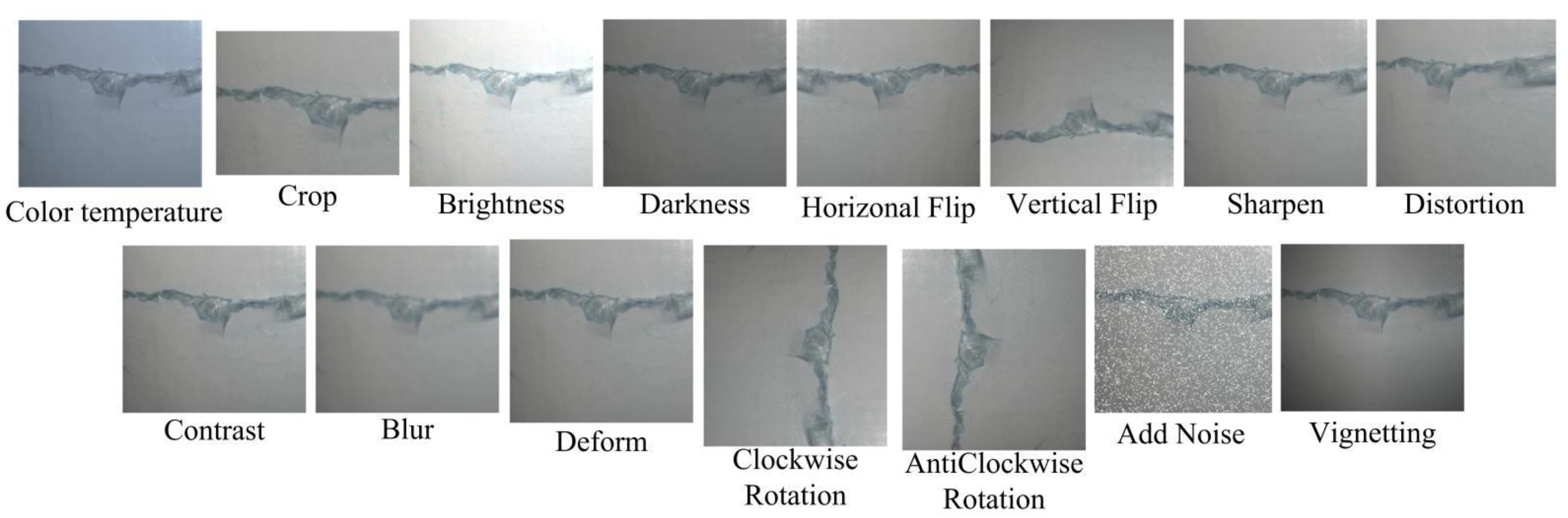
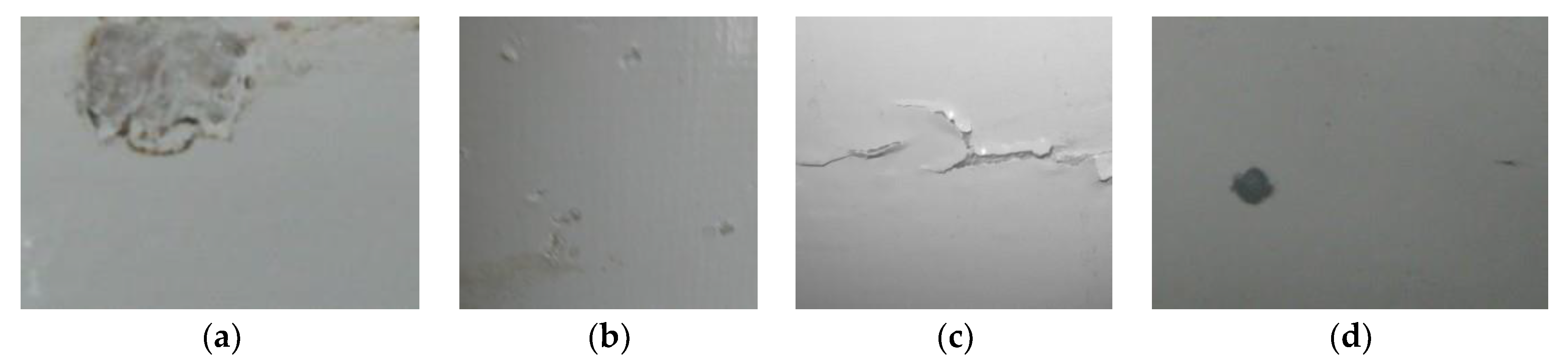
2.1. Image Preparation and Augmentation
2.2. Attention-Based MobileNetv1-YOLOv4
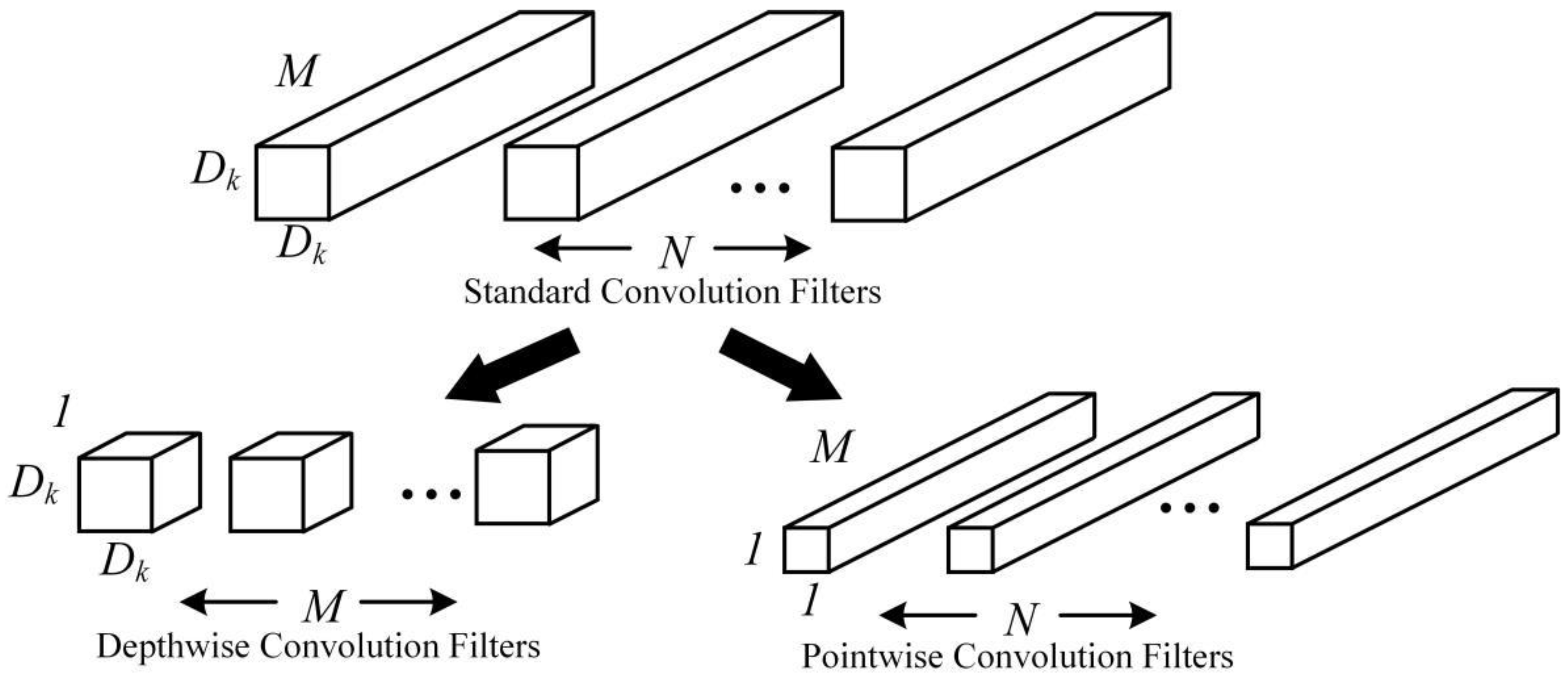
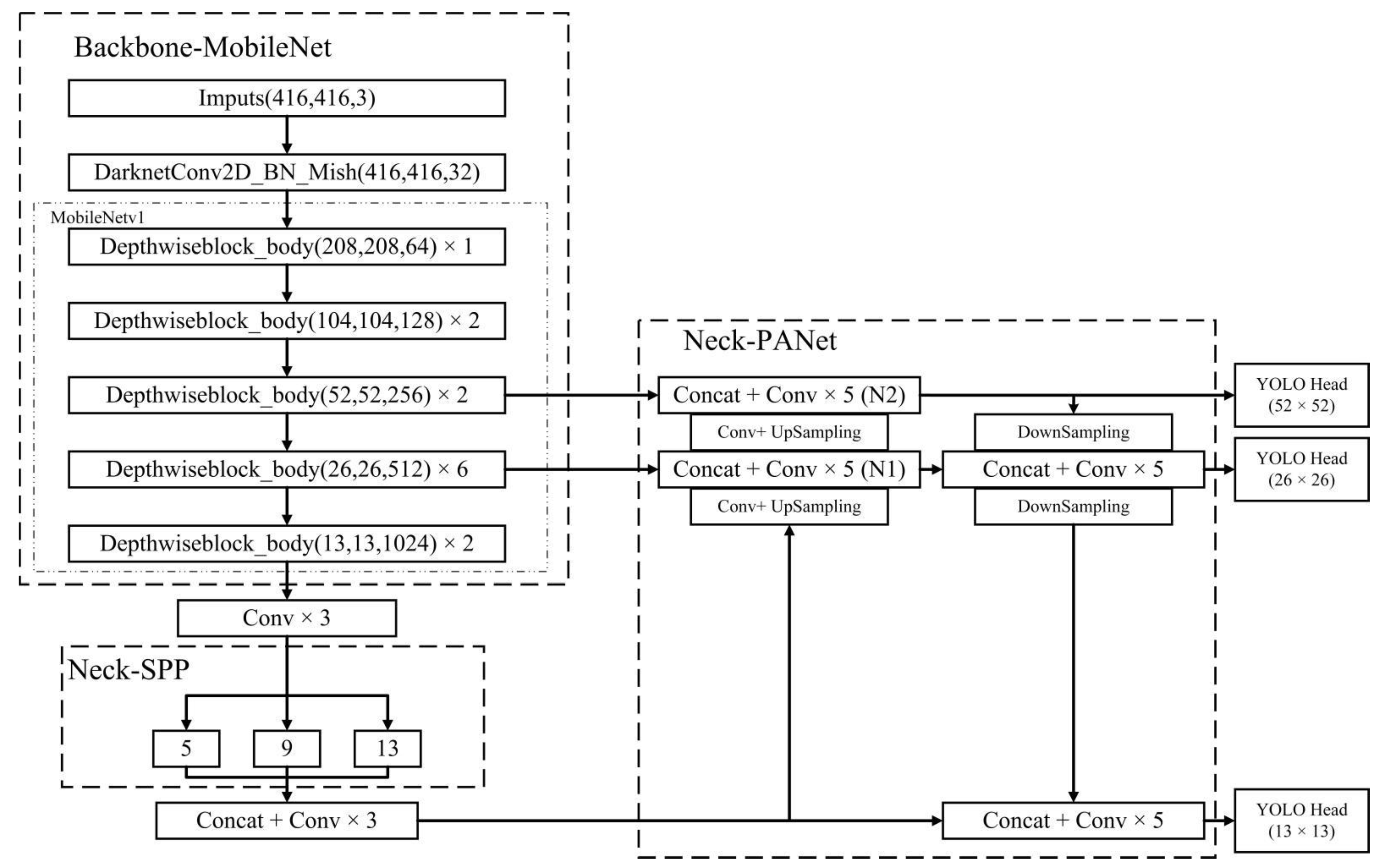
2.2.1. MobileNetv1-YOLOv4 Network
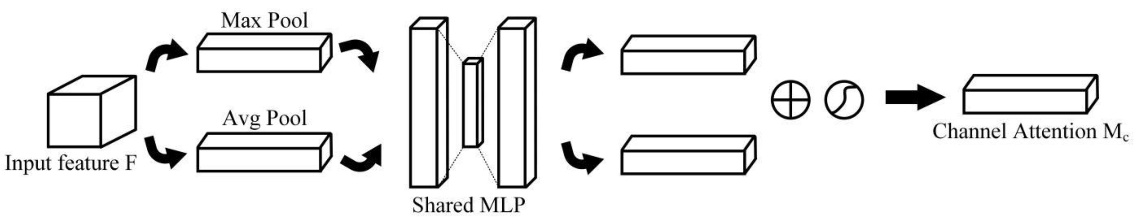
2.2.2. Attention-Based Modules
- SENet
- ECANet
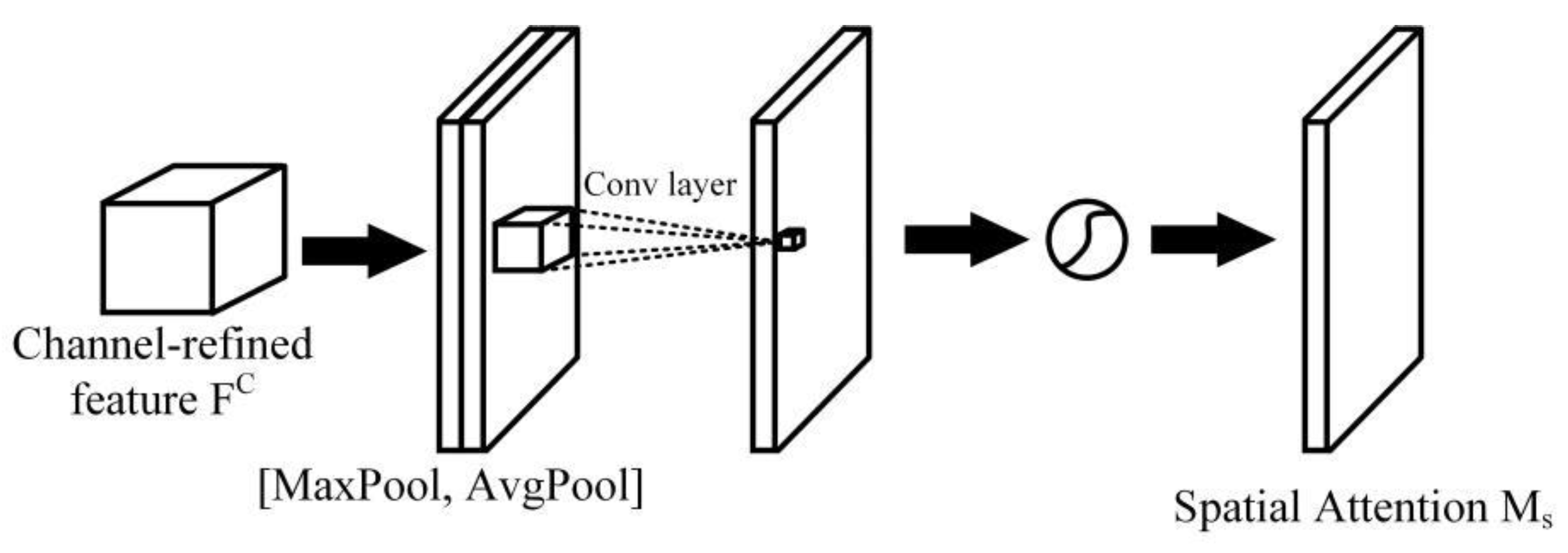
- CBAM
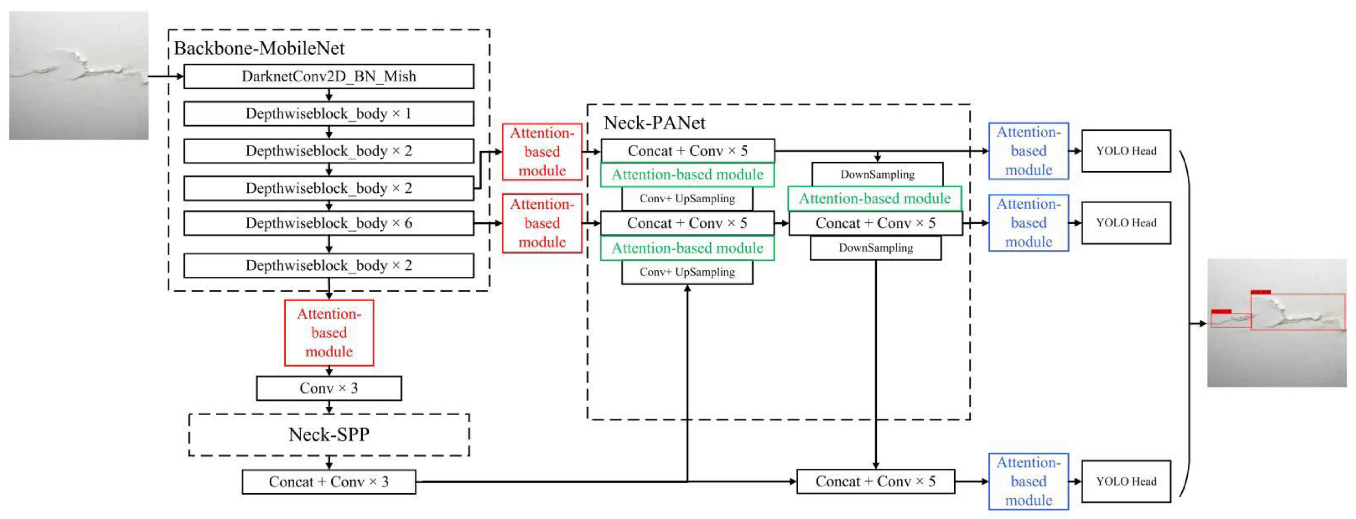
2.2.3. Attention-Based MobileNetv1-YOLOv4
2.2.4. Transfer Learning
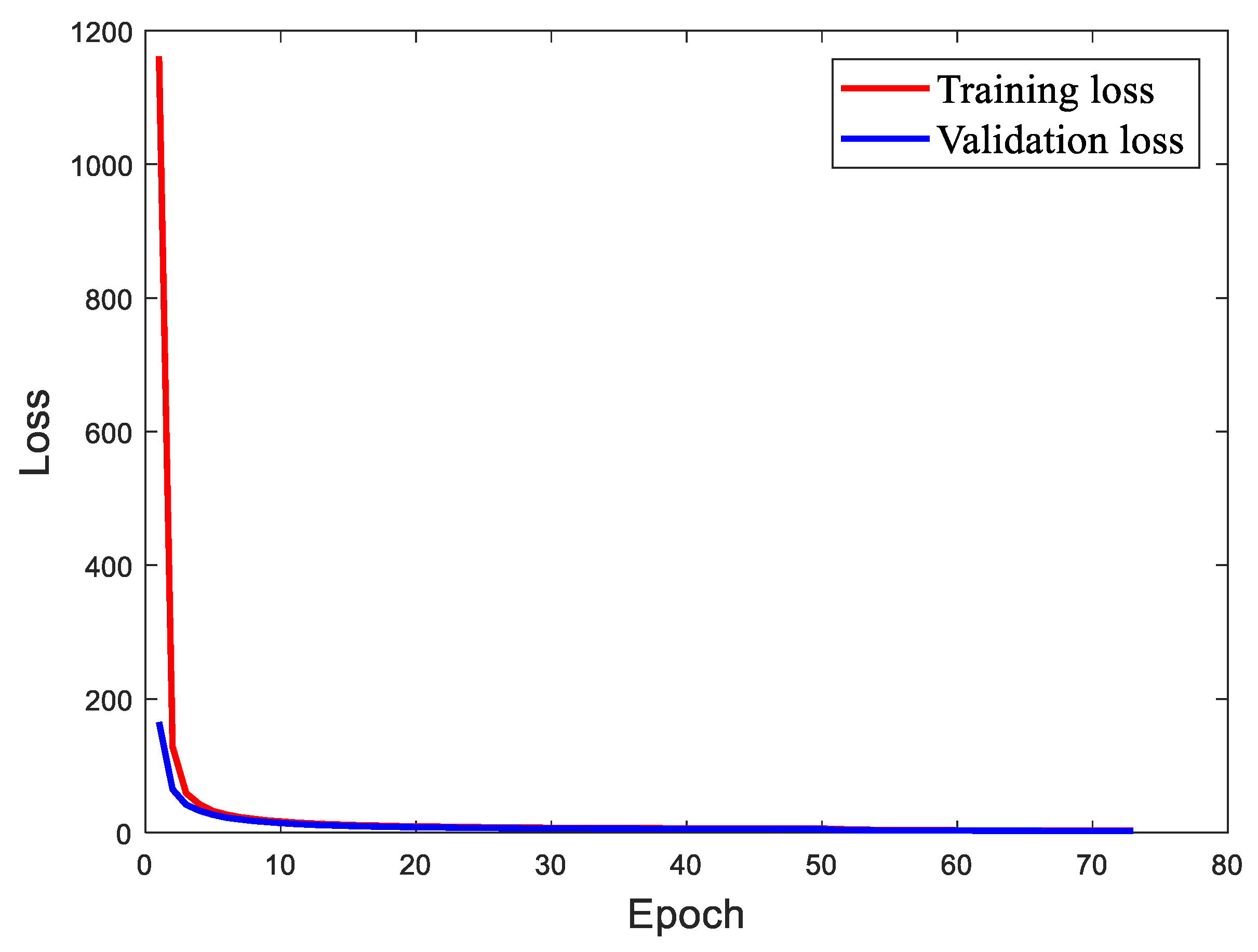
3. Results
4. Conclusions and Future Work
Author Contributions
Funding
Informed Consent Statement
Conflicts of Interest
References
- Ren, Z.; Verma, A.S.; Li, Y.; Teuwen, J.J.; Jiang, Z. Offshore wind turbine operations and maintenance: A state-of-the-art review. Renew. Sustain. Energy Rev. 2021, 144, 110886. [Google Scholar] [CrossRef]
- GWEC. Global Wind Report 2021; Global Wind Energy Council: Brussels, Belgium, 2022. [Google Scholar]
- Zhang, C.; Chen, H.P.; Huang, T.L. Fatigue damage assessment of wind turbine composite blades using corrected blade element momentum theory. Measurement 2018, 129, 102–121. [Google Scholar] [CrossRef]
- Habibi, H.; Howard, I.; Simani, S. Reliability Improvement of Wind Turbine Power Generation using Model-based Fault Detection and Fault Tolerant Control: A review. Renew. Energy 2019, 135, 877–896. [Google Scholar] [CrossRef]
- Márquez, F.P.G.; Chacón, A.M.P. A Review of Non-destructive Testing on Wind Turbines Blades. Renew. Energy 2020, 161, 998–1010. [Google Scholar] [CrossRef]
- Rizk, P.; Younes, R.; Ilinca, A.; Khoder, J. Defect Detection Using Hyperspectral Imaging Technology on Wind Turbine Blade. Remote Sens. Appl. Soc. Environ. 2021, 22, 100522. [Google Scholar]
- Zhao, Q.; Yuan, Y.; Sun, W.; Fan, X.; Fan, P.; Ma, Z. Reliability analysis of wind turbine blades based on non-Gaussian wind load impact competition failure model. Measurement 2020, 164, 107950. [Google Scholar] [CrossRef]
- Sierra-Perez, J.; Torres-Arredondo, M.A.; Gueemes, A. Damage and nonlinearities detection in wind turbine blades based on strain field pattern recognition. FBGs, OBR and strain gauges comparison. Compos. Struct. 2016, 135, 156–166. [Google Scholar] [CrossRef]
- Tian, S.; Yang, Z.; Chen, X.; Xie, Y. Damage Detection Based on Static Strain Responses Using FBG in a Wind Turbine Blade. Sensors 2015, 15, 19992–20005. [Google Scholar] [CrossRef] [PubMed]
- Bitkina, O.; Kang, K.W.; Lee, J.H. Experimental and theoretical analysis of the stress-strain state of anisotropic multilayer composite panels for wind turbine blade. Renew. Energy 2015, 79, 219–226. [Google Scholar] [CrossRef]
- Tang, J.; Soua, S.; Mares, C.; Gan, T.H. An experimental study of acoustic emission methodology for in service condition monitoring of wind turbine blades. Renew. Energy 2016, 99, 170–179. [Google Scholar] [CrossRef]
- Liu, Z.; Wang, X.; Zhang, L. Fault Diagnosis of Industrial Wind Turbine Blade Bearing Using Acoustic Emission Analysis. IEEE Trans. Instrum. Meas. 2020, 69, 6630–6639. [Google Scholar] [CrossRef]
- Habibi, H.; Cheng, L.; Zheng, H.; Kappatos, V.; Selcuk, C.; Gan, T.H. A dual de-icing system for wind turbine blades combining high-power ultrasonic guided waves and low-frequency forced vibrations. Renew. Energy 2015, 83, 859–870. [Google Scholar] [CrossRef]
- Muñoz, C.Q.G.; Jiménez, A.A.; Márquez, F.P.G. Wavelet transforms and pattern recognition on ultrasonic guides waves for frozen surface state diagnosis. Renew. Energy 2018, 116, 42–54. [Google Scholar] [CrossRef]
- Joshuva, A.; Sugumaran, V. A Lazy Learning Approach for Condition Monitoring of Wind Turbine Blade Using Vibration Signals and Histogram Features. Measurement 2020, 152, 107295. [Google Scholar] [CrossRef]
- Awadallah, M.; El-Sinawi, A. Effect and Detection of Cracks on Small Wind Turbine Blade Vibration Using Special Kriging Analysis of Spectral Shifts. Measurement 2019, 151, 107076. [Google Scholar] [CrossRef]
- Liu, Z.; Zhang, L.; Carrasco, J. Vibration analysis for large-scale wind turbine blade bearing fault detection with an empirical wavelet thresholding method. Renew. Energy 2020, 146, 99–110. [Google Scholar] [CrossRef]
- Muñoz, C.Q.; Márquez, F.P.; Tomás, J.M. Ice detection using thermal infrared radiometry on wind turbine blades. Measurement 2016, 93, 157–163. [Google Scholar] [CrossRef]
- Hwang, S.; An, Y.K.; Yang, J.; Sohn, H. Remote Inspection of Internal Delamination in Wind Turbine Blades using Continuous Line Laser Scanning Thermography. Int. J. Precis. Eng. Manuf.-Green Technol. 2020, 7, 699–712. [Google Scholar] [CrossRef]
- Du, Y.; Zhou, S.; Jing, X.; Peng, Y.; Wu, H.; Kwok, N. Damage detection techniques for wind turbine blades: A review. Mech. Syst. Signal Process. 2020, 141, 106445. [Google Scholar] [CrossRef]
- Xu, D.; Wen, C.; Liu, J. Wind turbine blade surface inspection based on deep learning and UAV-taken images. J. Renew. Sustain. Energy 2019, 11, 053305. [Google Scholar] [CrossRef]
- Long, X.Y.; Zhao, S.K.; Jiang, C.; Li, W.P.; Liu, C.H. Deep learning-based planar crack damage evaluation using convolutional neural networks. Eng. Fract. Mech. 2021, 246, 107604. [Google Scholar] [CrossRef]
- Cha, Y.J.; Choi, W.; Büyüköztürk, O. Deep Learning-Based Crack Damage Detection Using Convolutional Neural Networks. Comput.-Aided Civ. Infrastruct. Eng. 2017, 32, 361–378. [Google Scholar] [CrossRef]
- Gunturi, S.K.; Sarkar, D. Wind Turbine Blade Structural State Evaluation by Hybrid Object Detector Relying on Deep Learning Models. J. Ambient. Intell. Humaniz. Comput. 2021, 12, 8535–8548. [Google Scholar]
- Wang, L.; Zhang, Z.; Luo, X. A Two-Stage Data-Driven Approach for Image-Based Wind Turbine Blade Crack Inspections. IEEE/ASME Trans. Mechatron. 2019, 24, 1271–1281. [Google Scholar] [CrossRef]
- Wang, D.; Zhang, Y.; Yang, X. Image Recognition of Wind Turbines Blade Surface Defects Based on Mask-RCNN. In Advanced Intelligent Technologies for Industry; Springer: Singapore, 2022; pp. 573–584. [Google Scholar]
- Reddy, A.; Indragandhi, V.; Ravi, L.; Subramaniyaswamy, V. Detection of Cracks and damage in wind turbine blades using artificial intelligence-based image analytics. Measurement 2019, 147, 106823. [Google Scholar] [CrossRef]
- Pourkaramdel, Z.; Fekri-Ershad, S.; Nanni, L. Fabric defect detection based on completed local quartet patterns and majority decision algorithm. Expert Syst. Appl. 2022, 198, 116827. [Google Scholar] [CrossRef]
- Shih, K.H.; Chiu, C.T.; Lin, J.A.; Bu, Y.Y. Real-Time Object Detection with Reduced Region Proposal Network via Multi-Feature Concatenation. IEEE Trans. Neural Netw. Learn. Syst. 2020, 31, 2164–2173. [Google Scholar] [CrossRef]
- Redmon, J.; Divvala, S.; Girshick, R.; Farhadi, A. You Only Look Once: Unified, Real-Time Object Detection. In Proceedings of the 2016 IEEE Conference on Computer Vision and Pattern Recognition (CVPR), Las Vegas, NV, USA, 27–30 June 2016; pp. 779–788. [Google Scholar]
- Du, L.; Li, L.; Wei, D.; Mao, J. Saliency-Guided Single Shot Multibox Detector for Target Detection in SAR Images. IEEE Trans. Geosci. Remote Sens. 2020, 58, 3366–3376. [Google Scholar] [CrossRef]
- Tran, V.P.; Tran, T.S.; Lee, H.J.; Kim, K.D.; Baek, J.; Nguyen, T.T. One stage detector (RetinaNet)-based crack detection for asphalt pavements considering pavement distresses and surface objects. J. Civ. Struct. Health Monit. 2021, 11, 205–222. [Google Scholar] [CrossRef]
- Han, D.; Liu, Q.; Fan, W. A new image classification method using CNN transfer learning and web data augmentation. Expert Syst. Appl. 2018, 95, 43–56. [Google Scholar] [CrossRef]
- Redmon, J.; Farhadi, A. YOLO9000: Better, Faster, Stronger. In Proceedings of the IEEE Conference on Computer Vision & Pattern Recognition, Honolulu, HI, USA, 21–26 July 2017; pp. 6517–6525. [Google Scholar]
- Cai, K.; Miao, X.; Wang, W.; Pang, H.; Liu, Y.; Song, J. A modified YOLOv3 model for fish detection based on MobileNetv1v1 as backbone. Aquac. Eng. 2020, 91, 102117. [Google Scholar] [CrossRef]
- Hu, X.; Liu, Y.; Zhao, Z.; Liu, J.; Yang, X.; Sun, C.; Chen, S.; Li, B.; Zhou, C. Real-time detection of uneaten feed pellets in underwater images for aquaculture using an improved YOLO-V4 network. Comput. Electron. Agric. 2021, 185, 106135. [Google Scholar] [CrossRef]
- Hu, J.; Shen, L.; Sun, G. Squeeze-and-Excitation Networks. IEEE Trans. Pattern Anal. Mach. Intell. 2017, 42, 2011–2023. [Google Scholar] [CrossRef]
- Sultana, F.; Sufian, A.; Dutta, P. Advancements in Image Classification using Convolutional Neural Network. In Proceedings of the 2018 Fourth International Conference on Research in Computational Intelligence and Communication Networks, Kolkata, India, 22–23 November 2018. [Google Scholar]
- Wang, Q.; Wu, B.; Zhu, P.; Li, P.; Zuo, W.; Hu, Q. ECA-Net: Efficient Channel Attention for Deep Convolutional Neural Networks. In Proceedings of the 2020 IEEE/CVF Conference on Computer Vision and Pattern Recognition (CVPR), Seattle, WA, USA, 13–19 June 2020. [Google Scholar]
- Yang, X.; Zhang, Y.; Lv, W.; Wang, D. Image recognition of wind turbine blade damage based on a deep learning model with transfer learning and an ensemble learning classifier. Renew. Energy 2021, 163, 386–397. [Google Scholar] [CrossRef]
- Fang, Q.; Li, H.; Luo, X.; Ding, L.; Luo, H.; Rose, T.M.; An, W. Detecting non-hardhat-use by a deep learning method from far-field surveillance videos. Autom. Constr. 2018, 85, 1–9. [Google Scholar] [CrossRef]
- Kumar, S.; Gupta, H.; Yadav, D.; Ansari, I.A.; Verma, O.P. YOLOv4 algorithm for the real-time detection of fire and personal protective equipments at construction sites. Multimed. Tools Appl. 2021, 81, 22163–22183. [Google Scholar] [CrossRef]
- Alsaffar, M.; Jarallah, E.M. Isolation and characterization of lytic bacteriophages infecting Pseudomonas aeruginosa from sewage water. Int. J. PharmTech Res. 2016, 9, 220–230. [Google Scholar]


| Configuration | |
|---|---|
| Hardware environment | Operating System: Windows 10 |
| CPU: Inter E5-2650 v4 | |
| RAM: 64GB | |
| GPU: NVIDIA 1080Ti | |
| Software version | Pycharm2021.3.2 + Python 3.7.8 + CUDNN11.1.0 + CUDA11.1.74 |
| Training network parameters | Fixed image size: 416 × 416 |
| Batch size: 16 | |
| Optimizer: Adam | |
| Learning rate: 10−3 | |
| Decay rate: 5 × 10⁻⁴ | |
| Frozen epoch: 50 | |
| Unfrozen epoch: 50 |
| Algorithm | Parameter Size (MB) | Training Epochs | Training Time (s) | FPS | Precision (%) | Recall (%) | F1 Score | mAP (%) |
|---|---|---|---|---|---|---|---|---|
| FasterR-CNN [41] | 522.91 | 70 | 14,060 | 9.76 | 69.72 | 80.80 | 0.740 | 81.72 |
| YOLOv3 [24] | 236.32 | 73 | 7223 | 19.38 | 85.93 | 64.61 | 0.733 | 81.81 |
| YOLOv4 [35] | 245.53 | 63 | 6811 | 12.44 | 92.09 | 86.70 | 0.895 | 92.32 |
| YOLOv4-tiny [42] | 23.10 | 55 | 2802 | 40.58 | 93.11 | 31.83 | 0.418 | 67.43 |
| MobileNetv1-YOLOv4 | 48.42 | 73 | 6486 | 18.77 | 93.39 | 57.87 | 0.665 | 88.61 |
| Red Section | Green Section | Blue Section | ||||||||
|---|---|---|---|---|---|---|---|---|---|---|
| Basic | SENet | ECANet | CBAM | SENet | ECANet | CBAM | SENet | ECANet | CBAM | |
| Parameter size (MB) | 48.42 | 49.07 | 48.42 | 51.04 | 48.49 | 48.42 | 48.70 | 48.58 | 48.42 | 49.07 |
| FPS | 18.77 | 18.46 | 18.86 | 16.20 | 17.49 | 17.42 | 16.21 | 17.64 | 18.67 | 16.65 |
| Precision (%) | 93.39 | 96.62 | 96.96 | 97.26 | 98.46 | 97.52 | 97.58 | 97.08 | 96.28 | 96.61 |
| Recall (%) | 57.87 | 65.27 | 70.53 | 58.36 | 73.97 | 70.70 | 74.86 | 64.38 | 67.92 | 66.51 |
| F1 score | 0.665 | 0.738 | 0.795 | 0.655 | 0.820 | 0.790 | 0.823 | 0.735 | 0.770 | 0.758 |
| mAP (%) | 88.61 | 93.03 | 92.57 | 87.93 | 93.85 | 92.72 | 93.76 | 91.93 | 90.42 | 89.18 |
Publisher’s Note: MDPI stays neutral with regard to jurisdictional claims in published maps and institutional affiliations. |
© 2022 by the authors. Licensee MDPI, Basel, Switzerland. This article is an open access article distributed under the terms and conditions of the Creative Commons Attribution (CC BY) license (https://creativecommons.org/licenses/by/4.0/).
Share and Cite
Zhang, C.; Yang, T.; Yang, J. Image Recognition of Wind Turbine Blade Defects Using Attention-Based MobileNetv1-YOLOv4 and Transfer Learning. Sensors 2022, 22, 6009. https://doi.org/10.3390/s22166009
Zhang C, Yang T, Yang J. Image Recognition of Wind Turbine Blade Defects Using Attention-Based MobileNetv1-YOLOv4 and Transfer Learning. Sensors. 2022; 22(16):6009. https://doi.org/10.3390/s22166009
Chicago/Turabian StyleZhang, Chen, Tao Yang, and Jing Yang. 2022. "Image Recognition of Wind Turbine Blade Defects Using Attention-Based MobileNetv1-YOLOv4 and Transfer Learning" Sensors 22, no. 16: 6009. https://doi.org/10.3390/s22166009
APA StyleZhang, C., Yang, T., & Yang, J. (2022). Image Recognition of Wind Turbine Blade Defects Using Attention-Based MobileNetv1-YOLOv4 and Transfer Learning. Sensors, 22(16), 6009. https://doi.org/10.3390/s22166009