
LiDAR Echo Gaussian Decomposition Algorithm for FPGA Implementation


Abstract
:1. Introduction
- (i)
- proposing a new LiDAR echo Gaussian decomposition algorithm, which utilizes a pair of the Gaussian inflection points and eliminates the “false” inflection points using a judgment condition;
- (ii)
- paralleling the proposed algorithm with a FPGA hardware architecture;
- (iii)
- validating the accuracy and timeliness of the proposed method using two LiDAR datasets covering the Congo and Antarctic regions, respectively.
2. Improved Gaussian Decomposition Algorithm
2.1. Pre-Processing
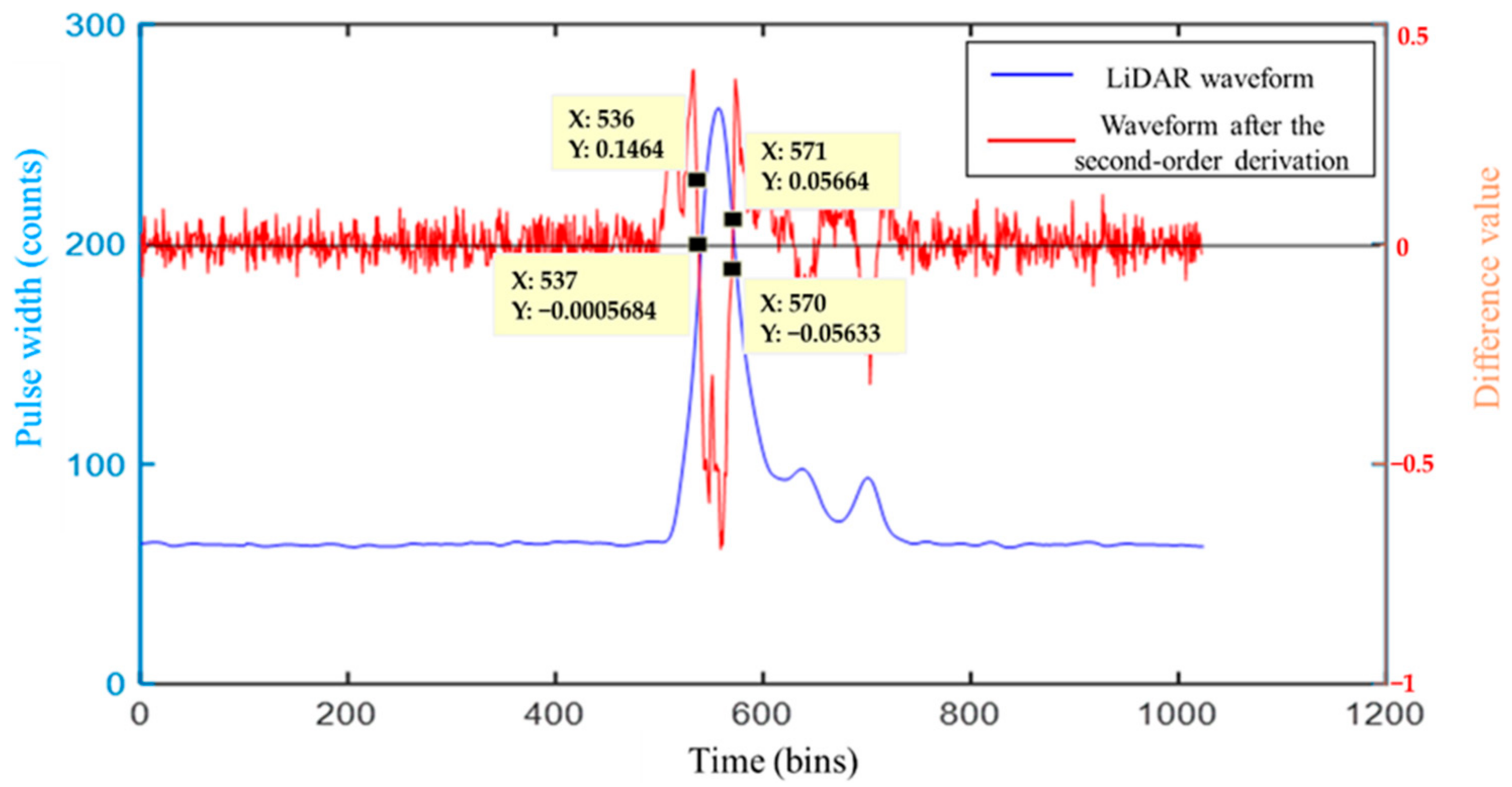
2.2. Inflection Point Coordinate Solution
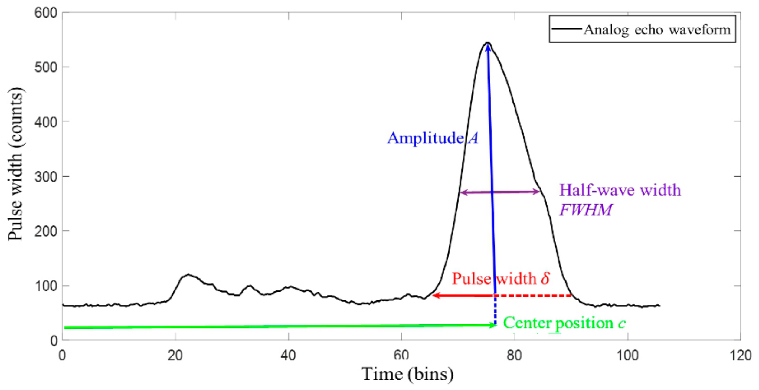
2.3. Gaussian Component Parameter Solution
2.4. Echo Component Location
3. FPGA Implementation for the Improved Gaussian Decomposition Algorithm
3.1. FPGA Overall Hardware Architecture
3.2. Submodule
3.2.1. Pre-Processing Module
- A.
- RAM data reading module
- B.
- Gaussian filter module
3.2.2. Inflection Point Coordinate Solution Module
- A.
- Second-order difference module
- B.
- Inflection point coordinate query module
- C.
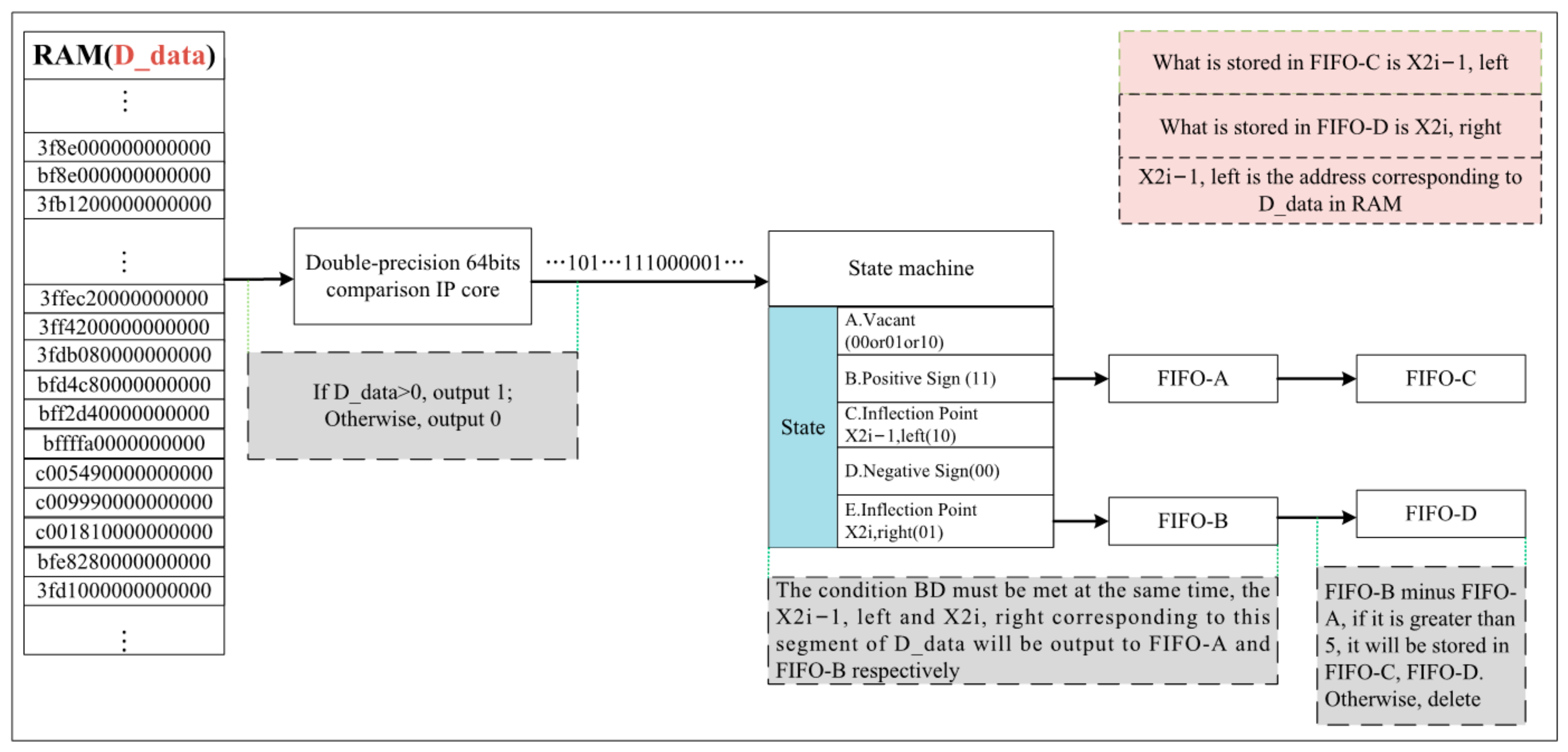
- State machine
- D.
- Inflection point coordinate calculation module
3.2.3. Gaussian Component Parameter Solving and Echo Component Positioning Module
- A.
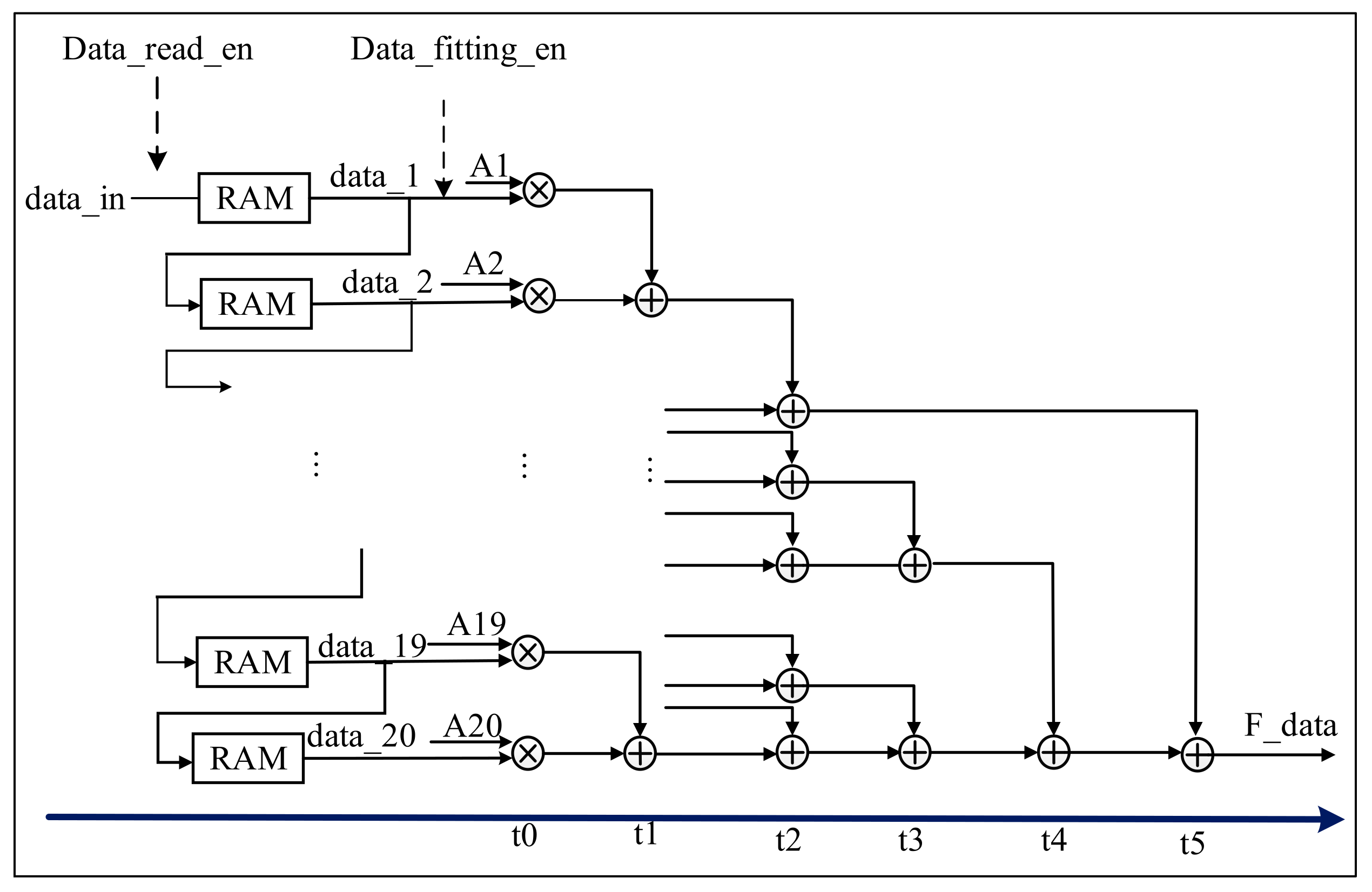
- Solving the amplitude ai
- B.
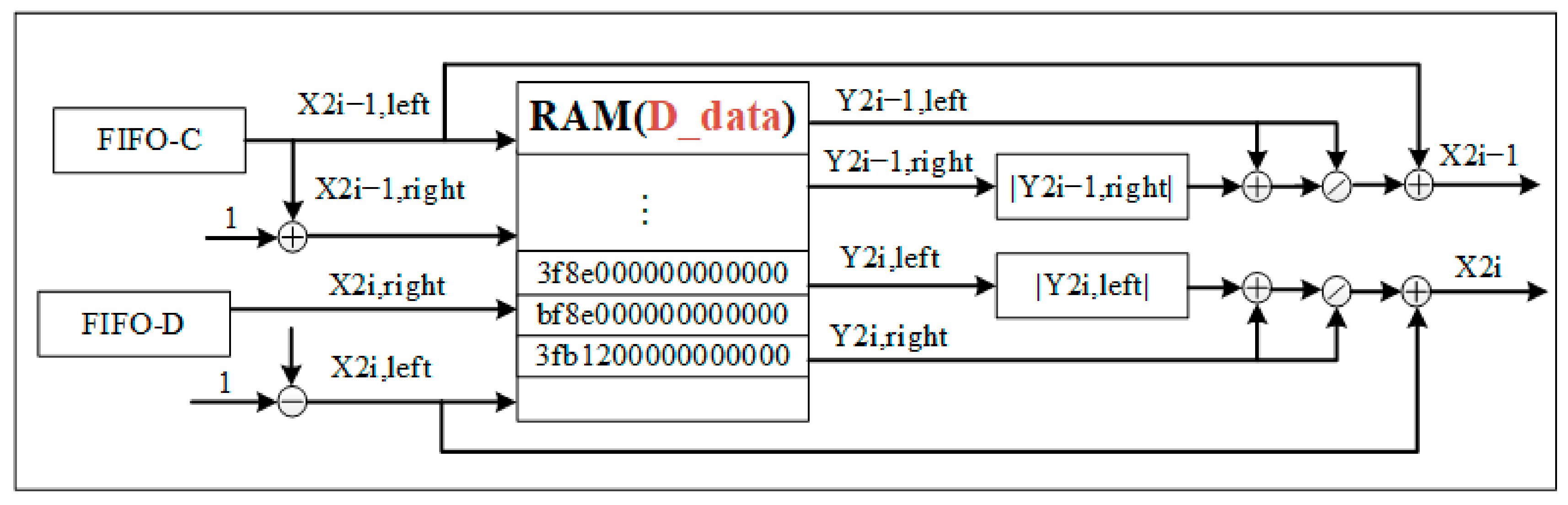
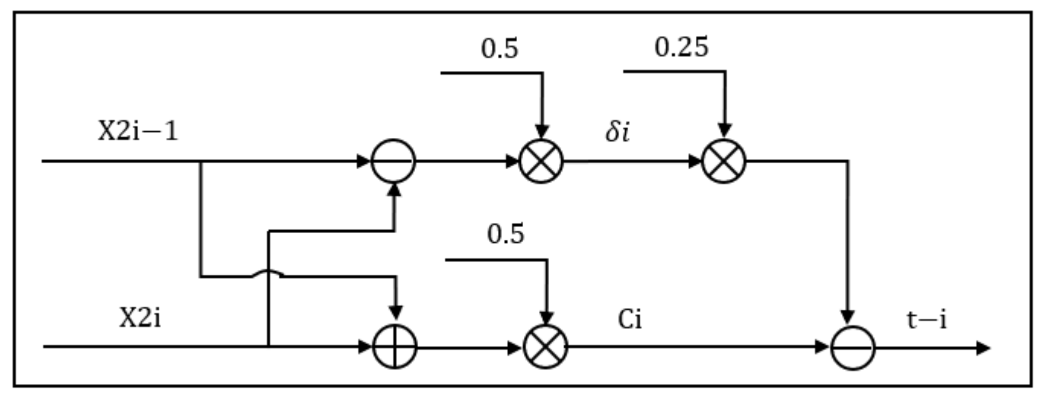
- Solving the center position ci, pulse width δi, and echo component positioning module
4. Experiments and Analysis
4.1. Data Sets
- (1)
- The Congo. The experimental data were collected from February to March 2016, and the flight area was Gabon, Africa. A Langley King Air B-200 aircraft was fitted with an LVIS installation for data collection, flying at an average ground elevation of 24 km. The nominal LVIS strip width was 1.5 km (200 mrad), and the nominal LVIS footprint diameter was 18 m (2.5 mrad). There are a total of 400,000 sets of data in each set, and the size of each data set is 1 × 1024.
- (2)
- Antarctica. The experiment was carried out in the Antarctic region is 2011. The LVIS was installed on NCAR’s G-V aircraft with an average ground altitude of 45 km. The nominal LVIS strip width was 2.7 km (200 mrad), and the nominal LVIS footprint diameter was 20 m (2.5 mrad). There are 700,000 sets of data in each set, and the size of each data set is 1 × 528.
- (3)
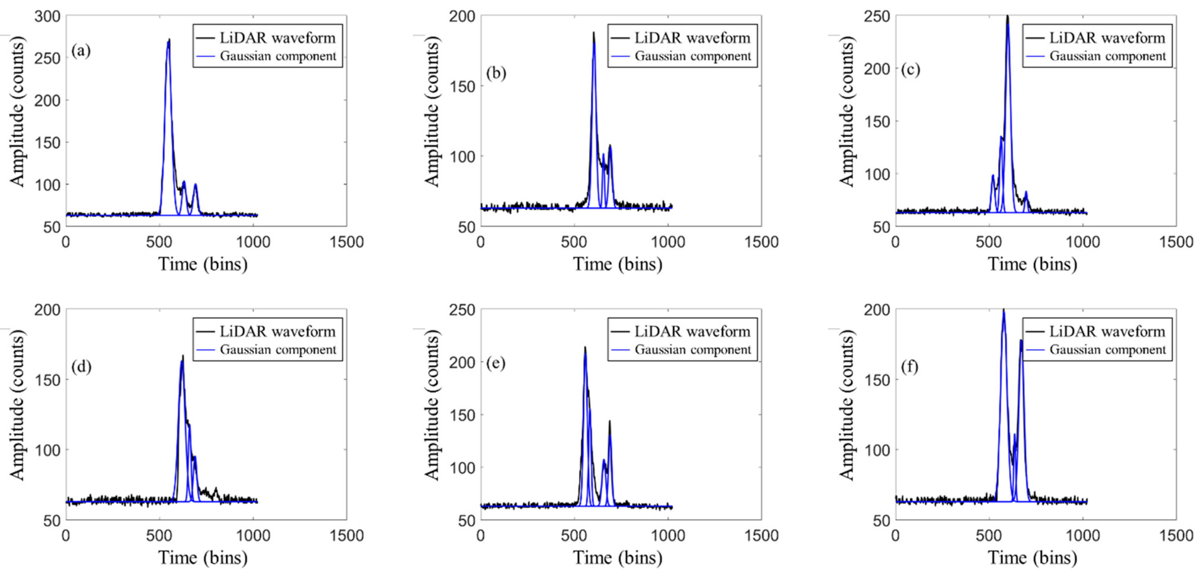
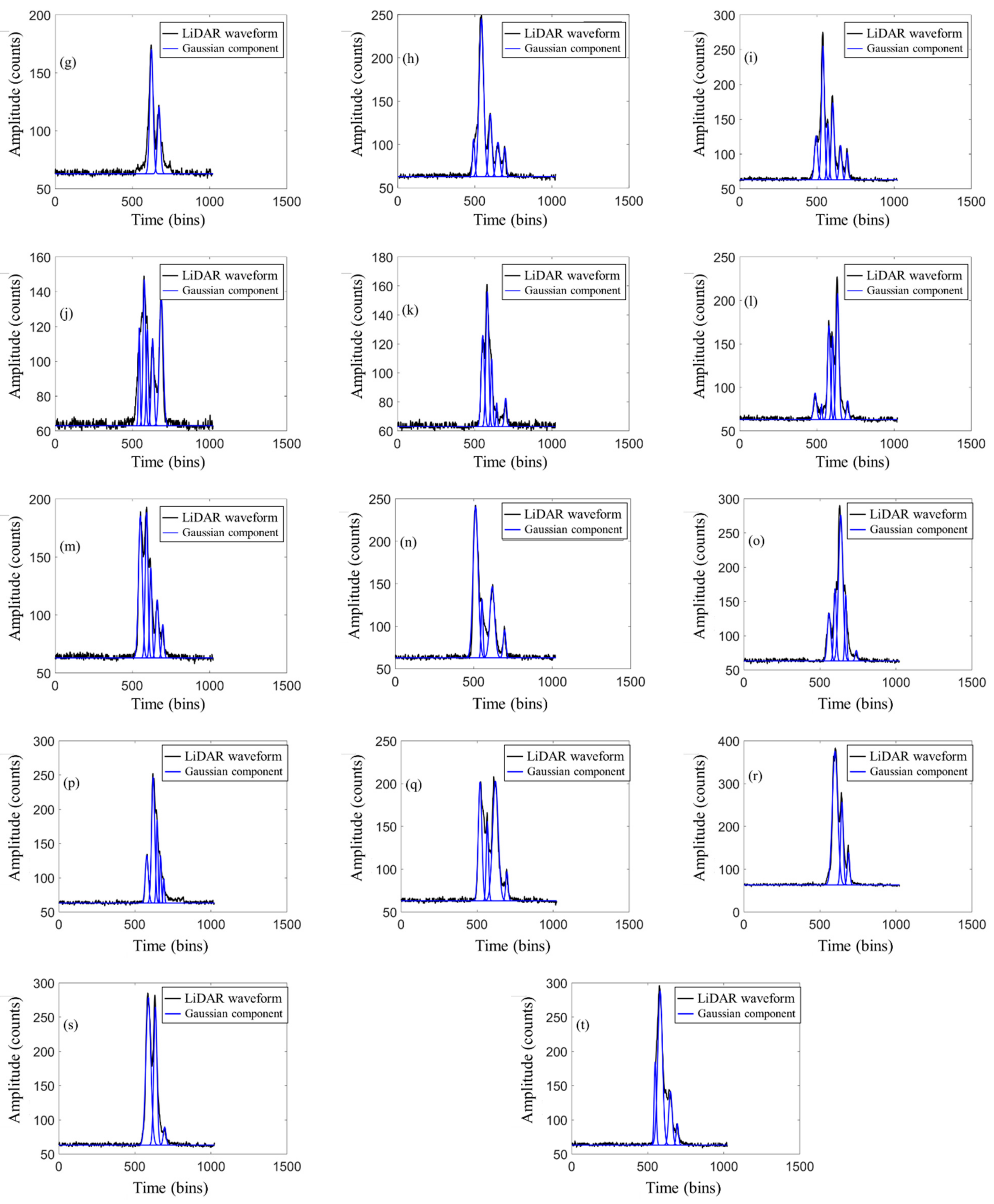
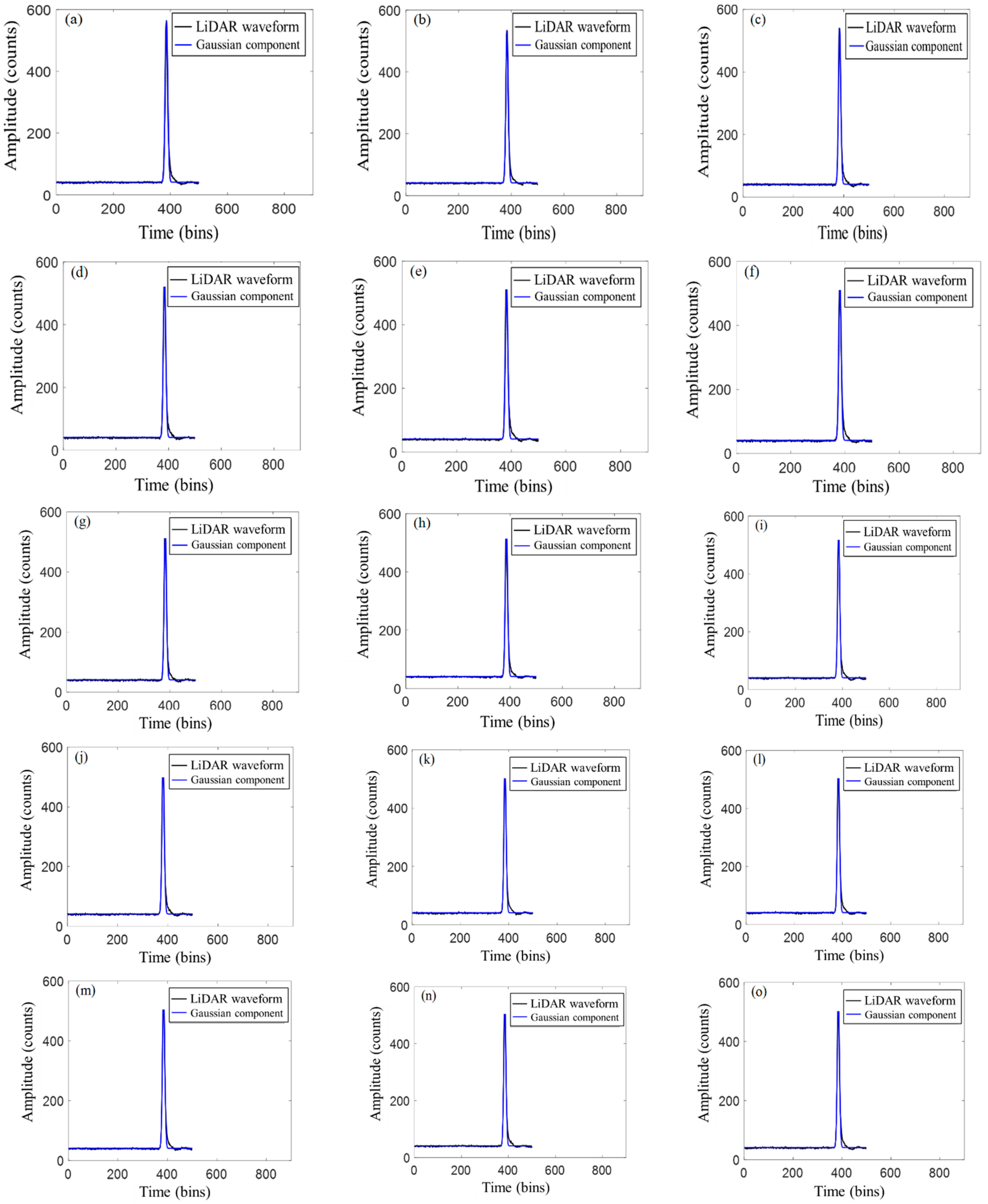
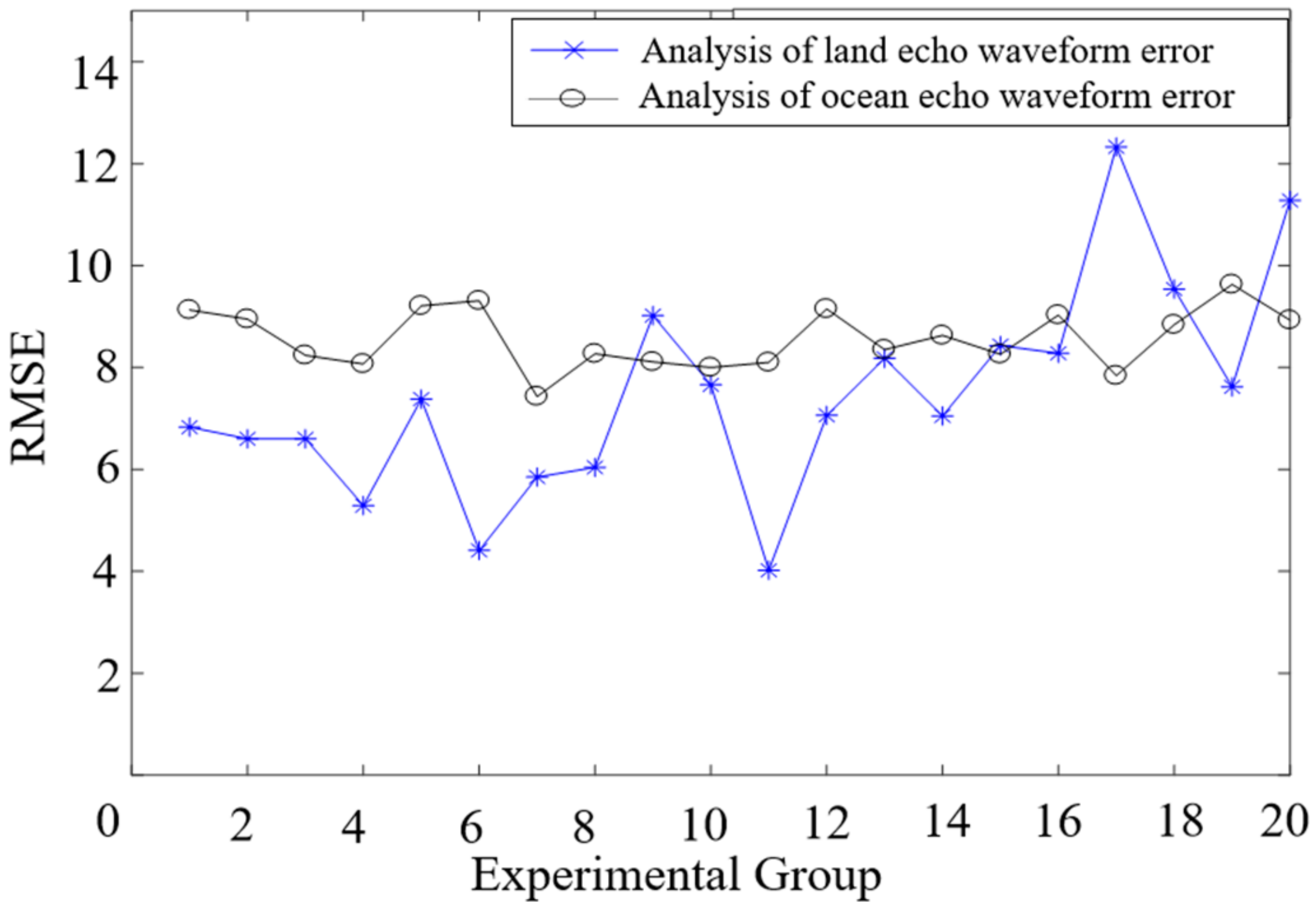
- Appendix A Figure A1 black waveform shows 20 sets of echo waveform data in the land area of Congo, while Appendix B Figure A2 black waveform shows 20 sets of echo waveform data in the ocean area of Antarctica. For the experiment, the echo waveform of the measurement area was decomposed and located, which is mainly divided into two categories: land and ocean. Vivado was used to test these 40 groups of data in order to realize the real-time reliability and accuracy of the algorithm.
- (4)
- In Appendix A Figure A1 black waveform, the abscissa is the sampling time point and the ordinate is the amplitude of the waveform. This paper includes as many various complex LiDAR echo waveforms as possible with different terrains, and the number of Gaussian components of each LiDAR echo ranged from 3 to 6.
- (5)
- In Appendix B Figure A2 black waveform, the abscissa is the sampling time point and the ordinate is the amplitude of the waveform. Due to the small influence factors, such as wind and waves, in the ocean area, the echo waveforms are simpler and have fewer Gaussian components.
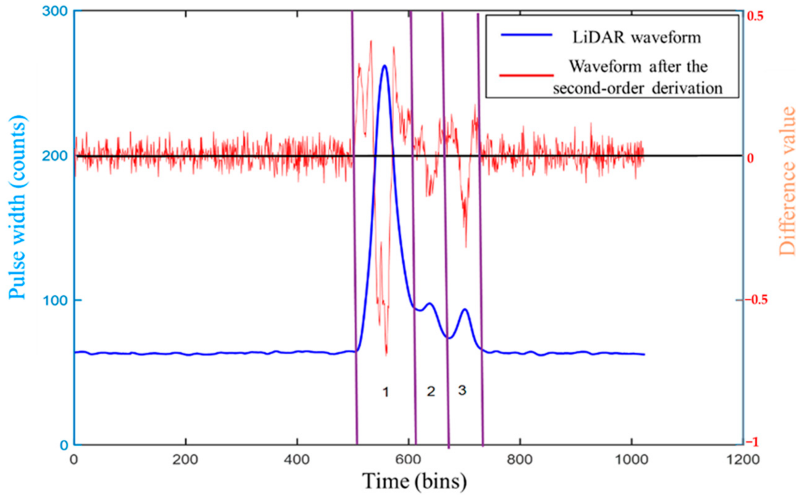
4.2. Echo Waveform Decomposition
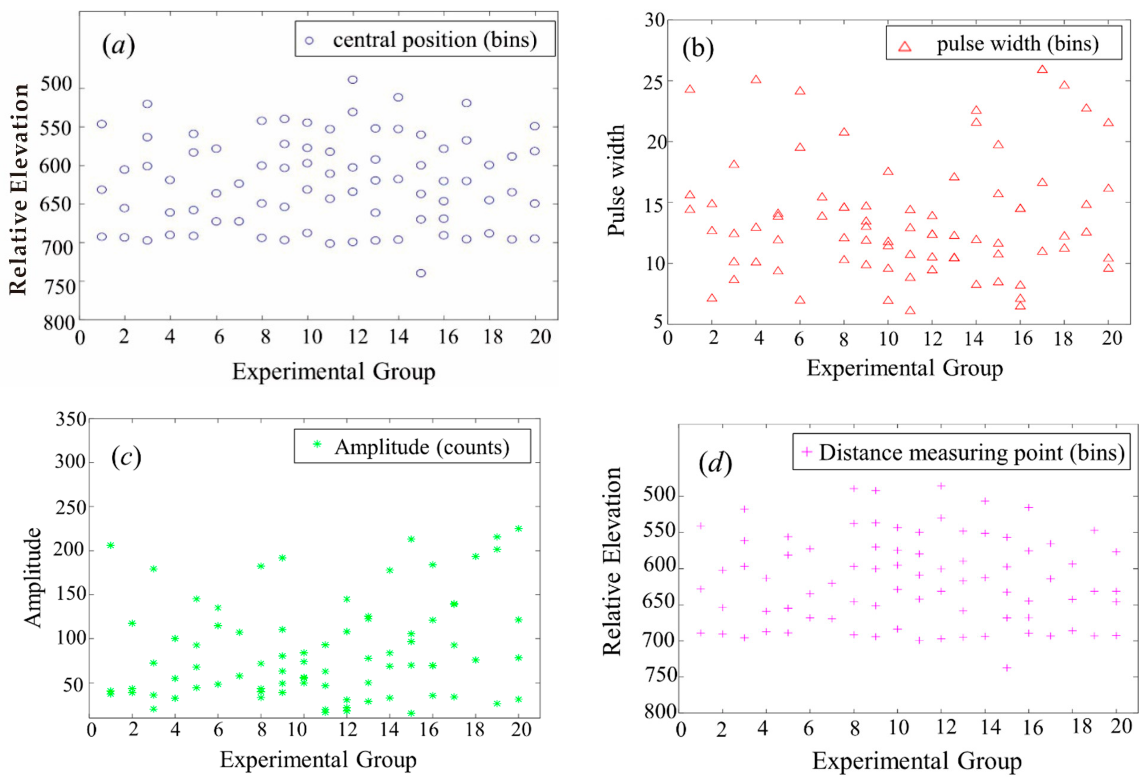
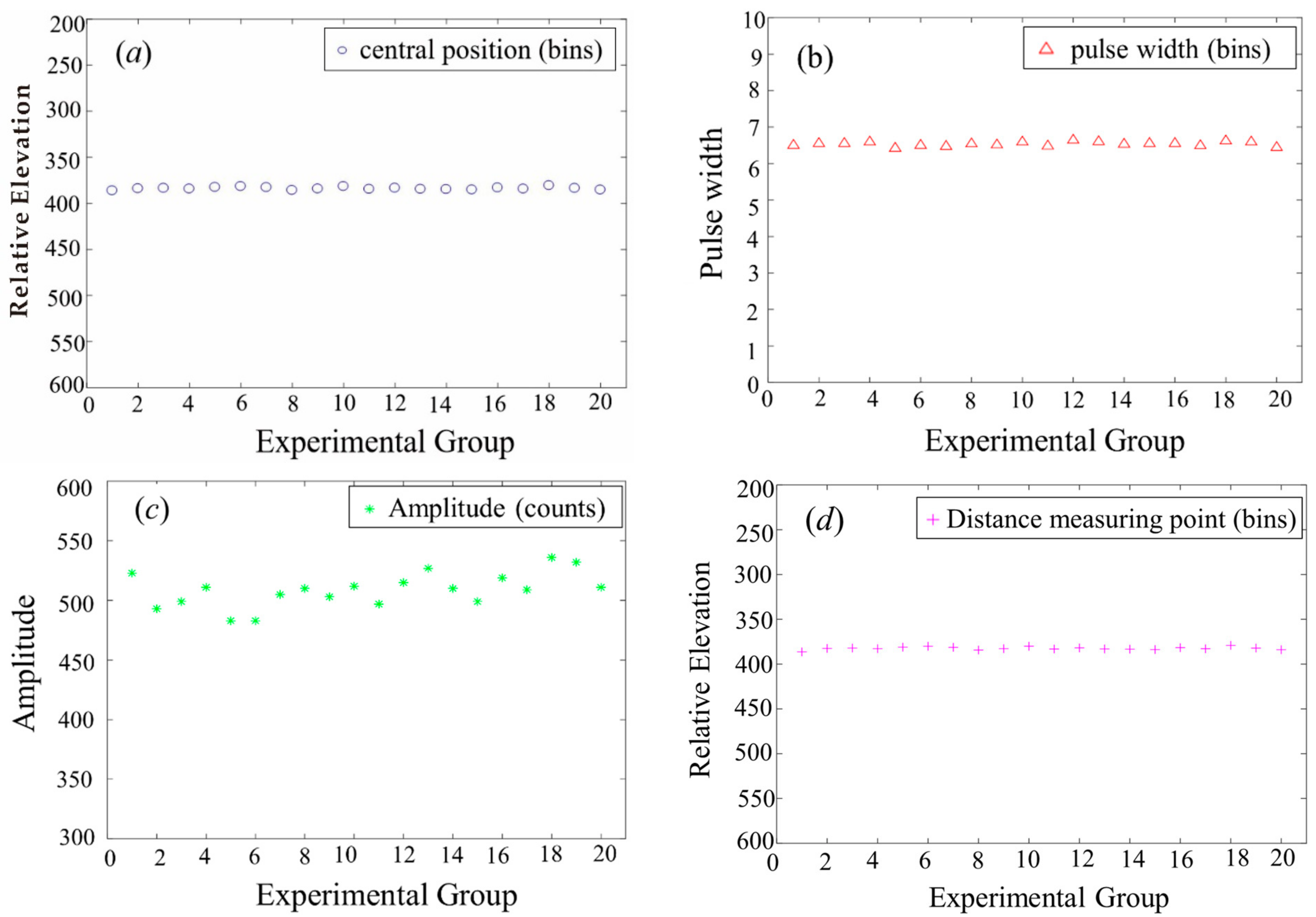
4.3. Error Analysis of Echo Waveform Decomposition
- (i)
- The deviation of the center position of the second Gaussian component in the first group of waveforms was 0.01, and the rest were the same;
- (ii)
- The pulse width error was generally 0.01;
- (iii)
- The amplitude error was relatively large, ranging from 0 to 0.16, but the amplitude value had no effect on the distance measurement point;
- (iv)
- Half of the distance measurement point had an error of 0.01—that is, the error was 0.0029 m—and the ratio of the order of magnitude to the distance measurement of this project was 10−2. Combining the above data, the result of FPGA operation basically met the requirements.
4.4. Processing Speed and Hardware Consumption Resource Situation
5. Conclusions
Author Contributions
Funding
Acknowledgments
Conflicts of Interest
Appendix A. LiDAR Waveform Data and LiDAR Echo Decomposition Waveform in the Congo Region
Appendix B. LiDAR Waveform Data and Decomposed Waveforms of Ocean LiDAR Waveforms in Antarctica

References
- Zhou, G.; Zhou, X. Imaging Principle, Technology and Application of Planar Array LiDAR; Wuhan University Press: Wuhan, China, 2018. [Google Scholar]
- Hofton, M.A.; Minster, J.B.; Blair, J.B. Decomposition of laser altimeter waveforms. IEEE Trans. Geosci. Remote Sens. 2000, 38, 1989–1996. [Google Scholar] [CrossRef]
- Abdallah, H.; Baghdadi, N.; Bailly, J.S.; Pastol, Y.; Fabre, F. Wa-LiD: A New LiDAR Simulator for Waters. IEEE Geosci. Remote Sens. Lett. 2012, 9, 744–748. [Google Scholar] [CrossRef] [Green Version]
- Cheng, F.; Wang, C.; Wang, J.; Tang, F.; Xi, X. Trend analysis of building height and total floor space in Beijing, China using ICESat/GLAS data. Int. J. Remote Sens. 2011, 32, 8823–8835. [Google Scholar] [CrossRef]
- Zhao, Q.; Li, H.; Li, Y. Gaussian Mixture Model with Variable Components for Full Waveform LiDAR Data Decomposition and RJMCM Algorithm. J. Surv. Mapp. 2015, 44, 1367–1377. [Google Scholar]
- Gong, P.; Li, Z.; Huang, H.; Sun, G.; Wang, L. ICESat GLAS Data for Urban Environment Monitoring. IEEE Trans. Geosci. Remote Sens. 2011, 49, 1158–1172. [Google Scholar] [CrossRef]
- Wang, X.; Cheng, X.; Gong, P.; Huang, H.; Li, Z.; Li, X. Earth science applications of ICESat/GLAS: A review. Int. J. Remote Sens. 2011, 32, 8837–8864. [Google Scholar] [CrossRef]
- Brodu, N.; Lague, D. 3D terrestrial lidar data classification of complex natural scenes using a multi-scale dimensionality criterion: Applications in geomorphology. ISPRS J. Photogramm. Remote Sens. 2012, 68, 121–134. [Google Scholar] [CrossRef] [Green Version]
- Kinzel, P.J.; Legleiter, C.J.; Nelson, J.M. Mapping river bathymetry with a small footprint green lidar: Applications and challenges. JAWRA J. Am. Water Resour. Assoc. 2013, 49, 183–204. [Google Scholar] [CrossRef]
- Zhuang, W.; Mountrakis, G. An accurate and computationally efficient algorithm for ground peak identification in large footprint waveform LiDAR data. ISPRS J. Photogramm. Remote Sens 2014, 95, 81–92. [Google Scholar] [CrossRef]
- Pan, Z.; Glennie, C.; Hartzell, P.; Fernandez-Diaz, J.C.; Legleiter, C.; Overstreet, B. Performance Assessment of High Resolution Airborne Full Waveform LiDAR for Shallow River Bathymetry. Remote Sens. 2015, 7, 5133–5159. [Google Scholar] [CrossRef] [Green Version]
- Li, W.; Niu, Z.; Li, J.; Chen, H.; Gao, S.; Wu, M.; Li, D. Generating pseudo large footprint waveforms from small footprint full-waveform airborne LiDAR data for the layered retrieval of LAI in orchards. Opt. Express 2016, 24, 10142–10156. [Google Scholar] [CrossRef]
- Liu, Y.; Deng, R.; Qin, Y.; Liang, Y. Data processing methods and applications of airborne LiDAR bathymetry. J. Remote Sens. 2017, 21, 982–995. [Google Scholar]
- Ma, H.; Zhou, W.; Zhang, L.; Wang, S. Decomposition of small-footprint full waveform LiDAR data based on generalized Gaussian model and grouping LM optimization. Meas. Sci. Technol. 2017, 28, 045203. [Google Scholar] [CrossRef]
- Bruggisser, M.; Roncat, A.; Schaepman, M.E.; Morsdorf, F. Retrieval of higher order statistical moments from full-waveform LiDAR data for tree species classification. Remote Sens. Environ. 2017, 196, 28–41. [Google Scholar] [CrossRef]
- Mountrakis, G.; Li, Y.A. Linearly approximated iterative Gaussian decomposition method for waveform LiDAR processing. ISPRS J. Photogramm. Remote Sens. 2017, 129, 200–211. [Google Scholar] [CrossRef]
- Budei, B.C.; St-Onge, B.; Hopkinson, C.; Audet, F.A. Identifying the genus or species of individual trees using a three-wavelength airborne lidar system. Remote Sens. Environ. 2018, 204, 632–647. [Google Scholar] [CrossRef]
- Song, S.; Gong, W.; Zhu, B.; Huang, X. Wavelength selection and spectral discrimination for paddy rice, with laboratory measurements of hyperspectral leaf reflectance. ISPRS J. Photogramm. Remote Sens. 2011, 66, 672–682. [Google Scholar] [CrossRef]
- Song, S.; Wang, B.; Gong, W.; Chen, Z.; Lin, X.; Sun, J.; Shi, S. A new waveform decomposition method for multispectral LiDAR. ISPRS J. Photogramm. Remote Sens. 2019, 149, 40–49. [Google Scholar] [CrossRef]
- Zhou, G.; Zhou, X.; Song, Y.; Xie, D.; Wang, L.; Yan, G.; Hu, M.; Liu, B.; Shang, W.; Gong, C.; et al. Design of supercontinuum laser hyperspectral light detection and ranging (LiDAR) (SCLaHS LiDAR). Int. J. Remote Sens. 2021, 42, 3731–3755. [Google Scholar] [CrossRef]
- Li, D.; Xu, L.; Li, L. Full-waveform LiDAR echo decomposition based on wavelet decomposition and particle swarm optimization. Meas. Sci. Technol. 2017, 28, 53–67. [Google Scholar] [CrossRef]
- Wagner, W.; Ullrich, A.; Ducic, V.; Melzer, T.; Studnicka, N. Gaussian decomposition and calibration of a novel small-footprint full-waveform digitising airborne laser scanner. ISPRS J. Photogramm. Remote Sens. 2006, 60, 100–112. [Google Scholar] [CrossRef]
- Heinzel, J.; Koch, B. Exploring full-waveform LiDAR parameters for tree species classification. Int. J. Appl. Earth Obs. Geoinf. 2011, 13, 152–160. [Google Scholar] [CrossRef]
- Zhang, X. Theory and Method of Airborne Lidar Measurement Technology; Wuhan University Press: Wuhan, China, 2007. [Google Scholar]
- Guo, K.; Xu, W.; Liu, Y.; He, X.; Tian, Z. Gaussian half-wavelength progressive decomposition method for waveform processing of airborne laser bathymetry. Remote Sens. 2017, 10, 35. [Google Scholar] [CrossRef] [Green Version]
- Gwenzi, D.; Lefsky, M.A. Modeling canopy height in a savanna ecosystem using spaceborne LiDAR waveforms. Remote Sens. Environ. 2014, 154, 338–344. [Google Scholar] [CrossRef]
- Muss, J.D.; Aguilar-Amuchastegui, N.; Mladenoff, D.J.; Henebry, G.M. Analysis of Waveform Lidar Data Using Shape-Based Metrics. IEEE Geosci. Remote Sens. Lett. 2013, 10, 106–110. [Google Scholar] [CrossRef] [Green Version]
- Zhou, G.; Zhang, R.; Liu, N.; Huang, J.; Zhou, X. On-board ortho-rectification for images based on an FPGA. Remote Sens. 2017, 9, 874. [Google Scholar] [CrossRef] [Green Version]
- Zhou, G. Urban High-Resolution Remote Sensing: Algorithms and Modelling; CRC Press: Boca Raton, FL, USA, 2020. [Google Scholar]
- Huang, J.; Zhou, G.; Zhou, X.; Zhang, R. A new FPGA architecture of FAST and BRIEF algorithm for on-board corner detection and matching. Sensors 2018, 18, 1014. [Google Scholar] [CrossRef] [PubMed] [Green Version]
- Zhou, G.; Deng, R.; Zhou, X.; Long, S.; Li, W.; Lin, G.; Li, X. Gaussian inflection point selection for LiDAR hidden echo signal decomposition. IEEE Geosci. Remote Sens. Lett. 2021, 19, 6502705. [Google Scholar] [CrossRef]
- Zhou, G.; Long, S.; Xu, J.; Zhou, X.; Song, B.; Deng, R.; Wang, C. Comparison analysis of five waveform decomposition algorithms for the airborne LiDAR echo signal. IEEE J. Sel. Top. Appl. Earth Obs. Remote Sens. 2021, 14, 7869–7879. [Google Scholar] [CrossRef]
- Zhou, G.; Li, C.; Liu, D.; Zhang, D. Overview of underwater transmission characteristics of oceanic LiDAR. IEEE J. Sel. Top. Appl. Earth Obs. Remote Sens. 2021, 14, 8144–8159. [Google Scholar] [CrossRef]


| Number | Echo Number | Central Location (Bins) | Pulse Width (Bins) | Amplitude (Counts) | RMSE |
|---|---|---|---|---|---|
| Figure A1a | 3 | 546.74 | 24.27 | 206.19 | 6.83 |
| 631.87 | 14.41 | 40.71 | |||
| 692.96 | 15.60 | 37.33 | |||
| Figure A1b | 3 | 605.78 | 14.87 | 117.70 | 6.60 |
| 655.82 | 7.10 | 38.72 | |||
| 693.81 | 12.64 | 43.41 |
| Number | Echo Number | Central Location (Bins) | Pulse Width (Bins) | Amplitude (Counts) | RMSE |
|---|---|---|---|---|---|
| Figure A1a | 3 | 546.74 | 24.27 | 206.03 | 6.83 |
| 631.88 | 14.40 | 40.71 | |||
| 692.96 | 15.59 | 37.34 | |||
| Figure A1b | 3 | 605.78 | 14.86 | 117.63 | 6.60 |
| 655.82 | 7.11 | 38.73 | |||
| 693.81 | 12.65 | 43.41 |
| Resources | Consumption | Percentage of Total Resources |
|---|---|---|
| FFs | 3389 | 0.9% |
| LUTs | 7215 | 60% |
| Memory LUTs | 39.5 | 7.9% |
| DSP48s | 32 | 3.5% |
Publisher’s Note: MDPI stays neutral with regard to jurisdictional claims in published maps and institutional affiliations. |
© 2022 by the authors. Licensee MDPI, Basel, Switzerland. This article is an open access article distributed under the terms and conditions of the Creative Commons Attribution (CC BY) license (https://creativecommons.org/licenses/by/4.0/).
Share and Cite
Zhou, G.; Zhou, X.; Chen, J.; Jia, G.; Zhu, Q. LiDAR Echo Gaussian Decomposition Algorithm for FPGA Implementation. Sensors 2022, 22, 4628. https://doi.org/10.3390/s22124628
Zhou G, Zhou X, Chen J, Jia G, Zhu Q. LiDAR Echo Gaussian Decomposition Algorithm for FPGA Implementation. Sensors. 2022; 22(12):4628. https://doi.org/10.3390/s22124628
Chicago/Turabian StyleZhou, Guoqing, Xiang Zhou, Jinlong Chen, Guoshuai Jia, and Qiang Zhu. 2022. "LiDAR Echo Gaussian Decomposition Algorithm for FPGA Implementation" Sensors 22, no. 12: 4628. https://doi.org/10.3390/s22124628
APA StyleZhou, G., Zhou, X., Chen, J., Jia, G., & Zhu, Q. (2022). LiDAR Echo Gaussian Decomposition Algorithm for FPGA Implementation. Sensors, 22(12), 4628. https://doi.org/10.3390/s22124628