
Comprehensive Analysis of Applied Machine Learning in Indoor Positioning Based on Wi-Fi: An Extended Systematic Review †


Abstract
:1. Introduction
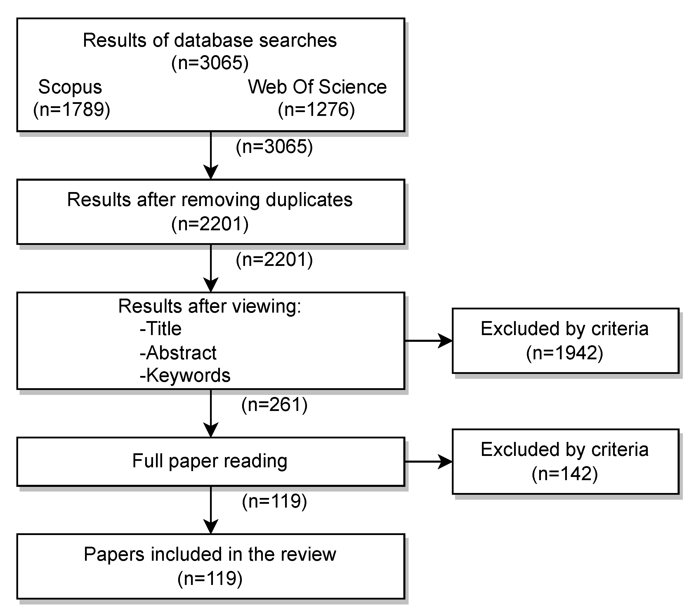
- The current work extends the analyzed period to the last five years, analysing a total of 119 published research works, 57 more than in [11];
- An analysis of solutions based on Artificial Neural Networks (ANN), Suport Vector Machines (SVM), and Random Forest (RF) is included;
- A comprehensive analysis of the most widely used public datasets (radio maps) and how they have been integrated in experiments performed by the research community;
- A discussion of the size of the operational areas considered in experiments performed in the reviewed works;
- Extended context, discussion, and conclusions.
2. Related Work
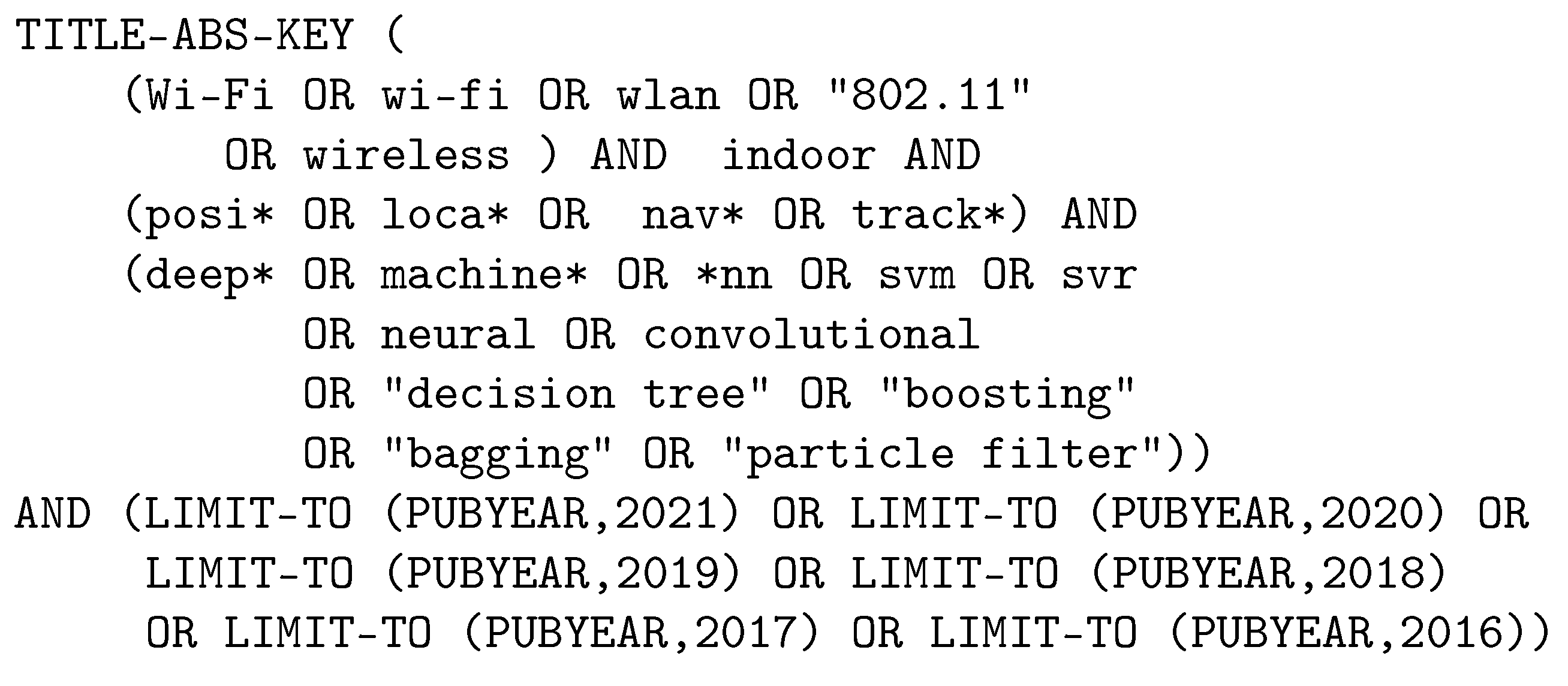
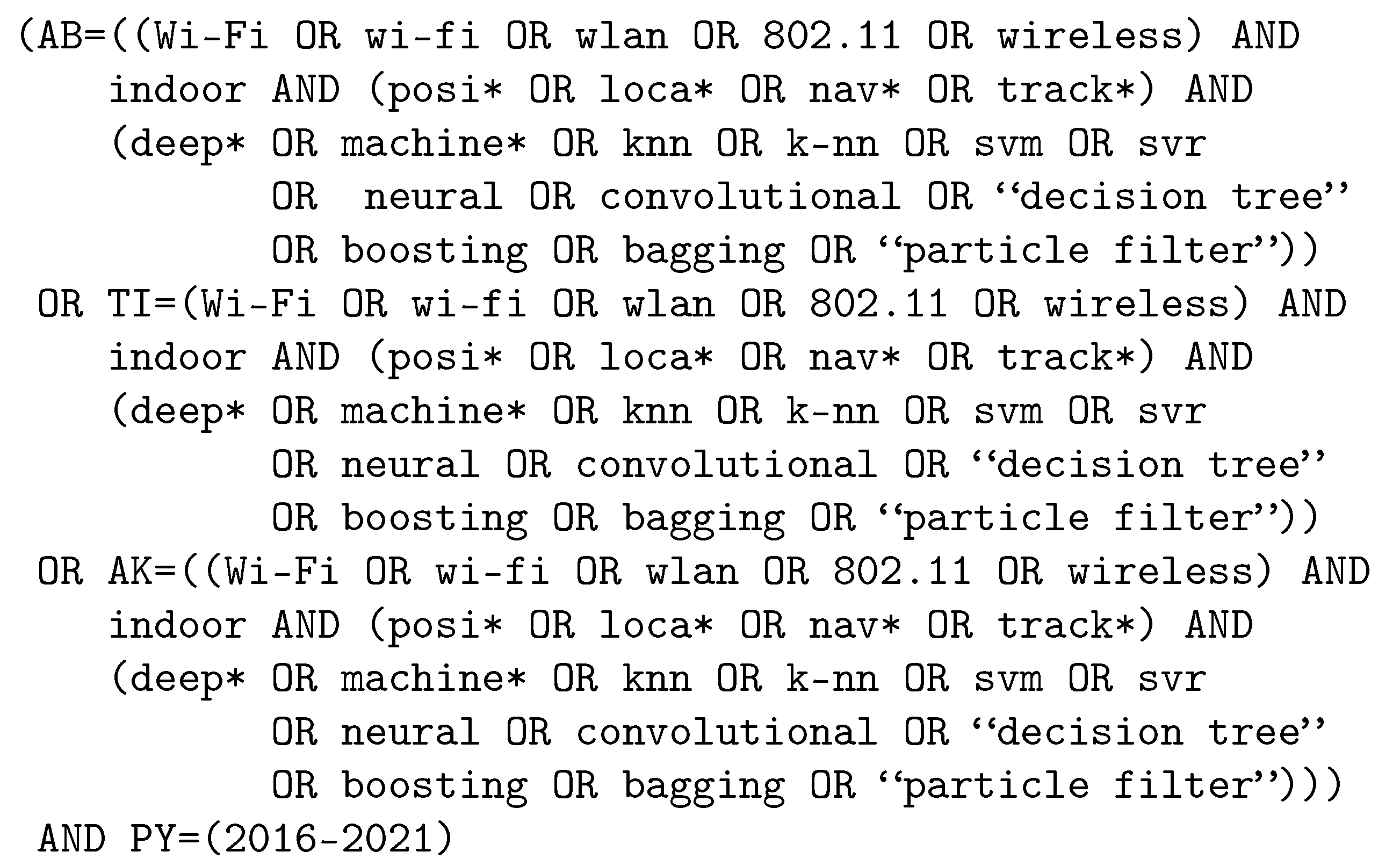
3. Methodology
- RQ1.
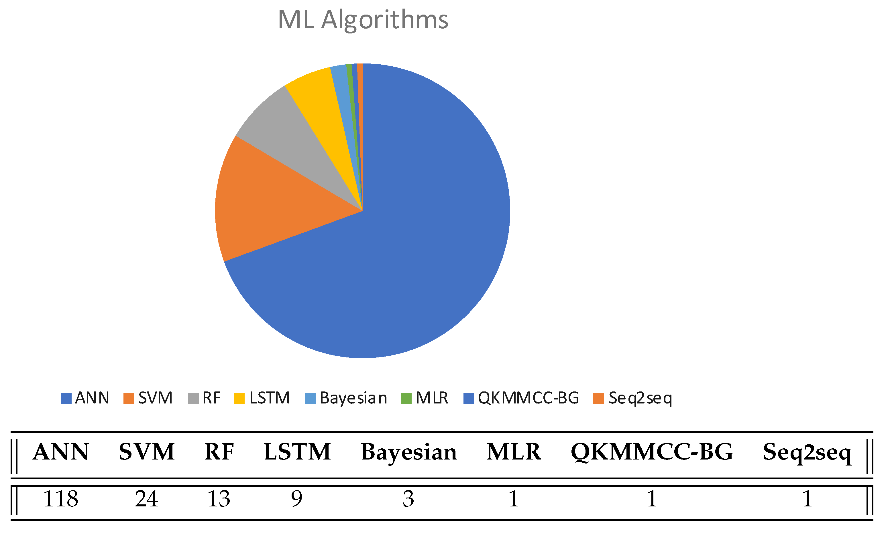
- Which machine learning algorithms provide the best results in Wi-Fi-based indoor positioning?
- RQ2.
- What kind of Wi-Fi signal parameters provide the best results?
- RQ3.
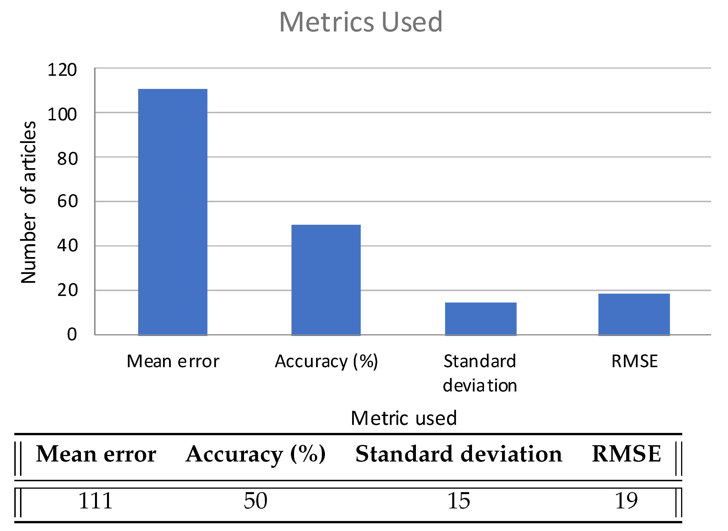
- What are the most commonly used metrics in indoor positioning studies?
- RQ4.
- Are there substantial differences between simulated and experimental studies?
- RQ5.
- Which public radio signal maps are the most commonly used in simulations?
- IC1.
- Written in English
- IC2.
- Coming from a conference or journal article
- IC3.
- Dealing with Wi-Fi-based positioning
- IC4.
- Positioning through Machine Learning algorithms
- IC5.
- Published between 2016 to 2021
- EC1.
- Workshops and book chapters
- EC2.
- Positioning that is not 100% Wi-Fi or is based on Sensor Fusion
- EC3.
- Positioning that has part of the work outdoors
- EC4.
- Positioning based on classic multilateration (TOA, AOA, etc.)
- EC5.
- Positioning that uses a KNN-based algorithm or Particle Filter, as this is not considered Machine Learning
4. Results
- Features not explained in the articles appear as .
- Articles that include different experiments and/or simulations are grouped together.
- Articles that do not display a clear metric are marked in the column oError (Other Errors).
- Articles that are based on or use algorithms different from the main one are marked in the column sAlg (Secondary Algorithm)
5. Discussion
5.1. Methods: Algorithms and Machine Learning Models
5.1.1. Neural Networks
5.1.2. Support Vector Machines
5.1.3. Random Forest
5.1.4. Comparison of Models
5.2. Types of Wi-Fi Signal Parameters Used
5.3. Evaluation Metrics
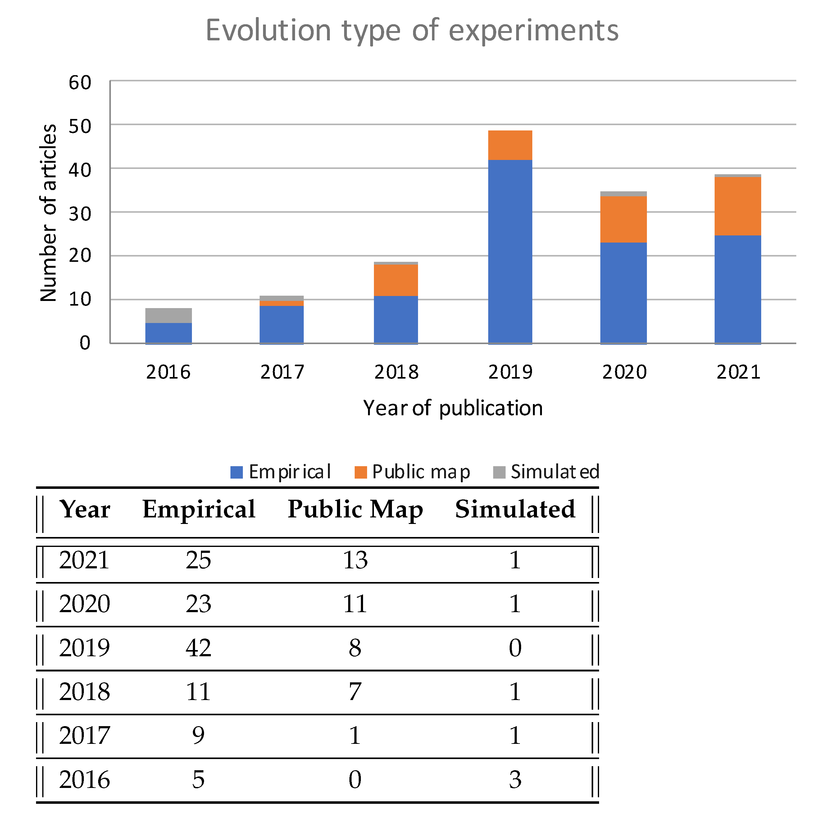
5.4. Experimental and Full Simulated Results
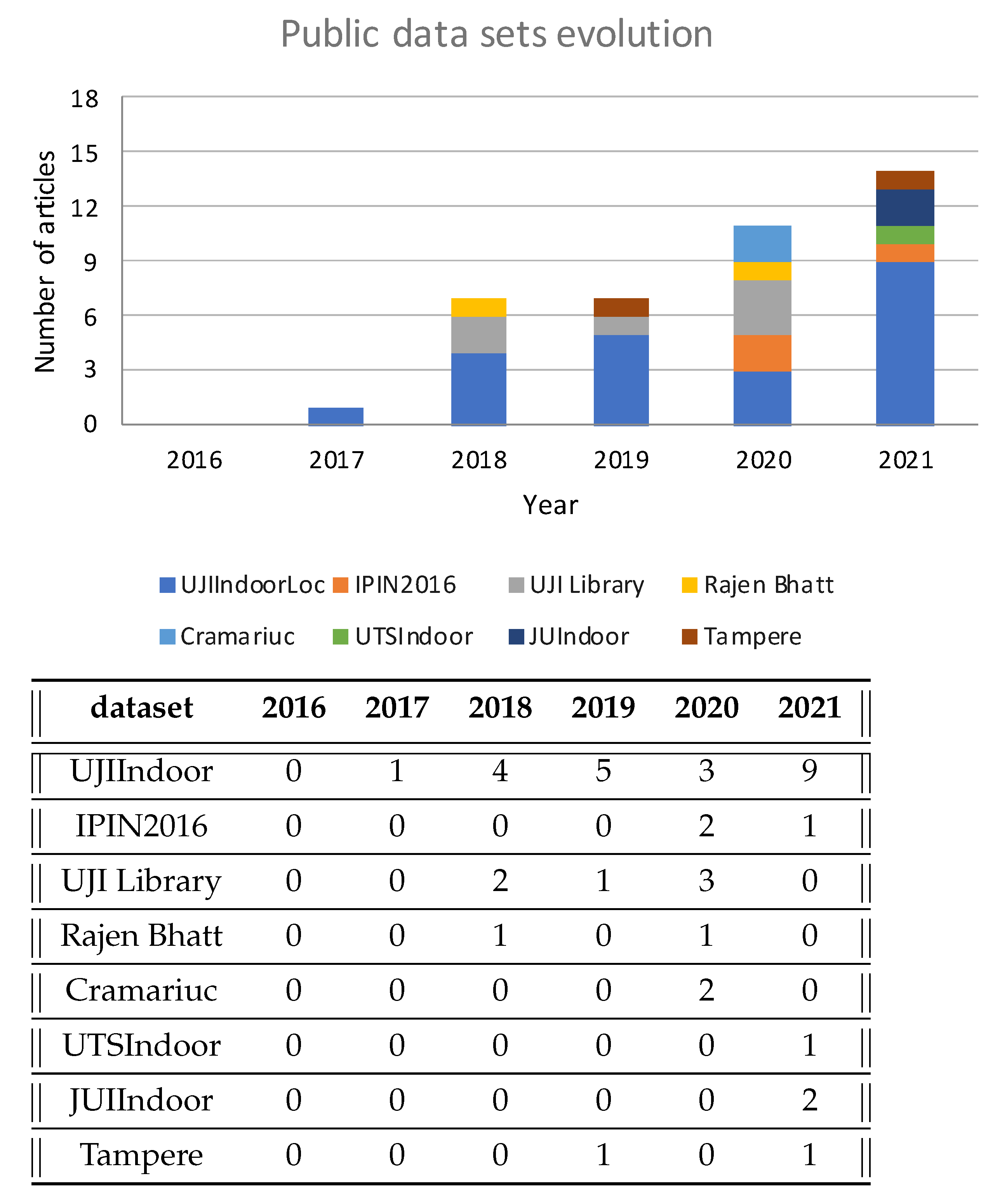
5.5. Most Widely Used Public Datasets
UJIIndoor Results Analysis
5.6. Experimental Scenarios
6. Conclusions
Author Contributions
Funding
Institutional Review Board Statement
Conflicts of Interest
Abbreviations
| ANN | Artificial Neural Networks |
| AoA | Angle of Arrival |
| AP | Access Point |
| BPNN | Back Propagation Neural Network |
| CapsNet | Capsule Neural Network |
| CNN | Convolutional Neural Networks |
| CSI | Channel State Information |
| DBN | Deep Belief Network |
| DNN | Deep Neural Networks |
| DQN | Deep Q-Networks |
| DRL | Deep reinforcement learning |
| ELM | Extreme learning machine |
| GNSS | Global Navigation Satellite Systems |
| MLP | Multilayer Perceptron |
| MSE | Mean Squared Error |
| NN | Neural Network |
| PoA | Phase of Arrival |
| RF | Random Forest |
| RMSE | Root Mean Squared Error |
| RNN | Recurrent Neural Networks |
| RSSI | Received Signal Strength Indicator |
| SDA | Stacked Denoising Autoencoders |
| SMN | Single Multiplicative Neuron |
| SNR | Signal-to-Noise Ratio |
| SVM | Suport Vector Machines |
| ToF | Time Of Flight |
| VAE | Variational Autoencoder |
Appendix A. Full Features of Reviewed Articles

| Art | Year | Est | AP | rPoint | fMap | fmRoom | mAlg | sAlg | mError | oError | sType |
|---|---|---|---|---|---|---|---|---|---|---|---|
| [41] | 2021 | pMap | 168 | 57 | IPIN2016 | N | DRL | RSSI | |||
| pMap | 589 | 1452 | UTSIndoorLoc | Y | DRL | RSSI | |||||
| pMap | 520 | 993 | UJIIndoorLoc | Y | DRL | Only Building B1 | RSSI | ||||
| [22] | 2021 | pMap | 96 | 80 | JUIndoorLoc | Y | BayesNet | Dempster–Shafer | Accuracy = 80% between 3 and 3.6 m | RSSI | |
| pMap | 520 | 993 | UJIIndoorLoc | Y | BayesNet | Accuracy = 98% in 2 m | RSSI | ||||
| [87] | 2021 | exp | 7 | 116 | 1052 | Y | SISAE (NN) | std = 1.34 m | RSSI | ||
| [44] | 2021 | exp | 1 | 32 | N | CNN | CSI | ||||
| exp | 1 | 45 | 40 | N | CNN | CSI | |||||
| exp | 1 | 66 | Y | CNN | CSI | ||||||
| exp | 1 | 15 | 32 | N | CNN | CSI | |||||
| [45] | 2021 | sim | 15 | 158 | 1160 | Y | ASDELM (ELM) | Accuracy = 85,90% in 1 m | CSI | ||
| exp | 22 | 47 | 384 | Y | ASDELM (ELM) | Accuracy = 77% in 1 m | CSI | ||||
| [88] | 2021 | pMap | 520 | 993 | UJIIndoorLoc | Y | DNNIP | Accuracy = 89% building and floor | RSSI | ||
| [80] | 2021 | pMap | 520 | 993 | UJIIndoorLoc | Y | CHISEL (CNN) | autoencoder | Accuracy = 99.6% building, 83.97% floor | RSSI | |
| [46] | 2021 | exp | 1 | 40 | 131.3 | Y | BPNN | adaptive genetic algorithm | Accuracy = 90.47% in 4 m | CSI | |
| [30] | 2021 | pMap | 520 | 993 | UJIIndoorLoc | Y | NNELILS (NN) | 67% to 78% localization accuracies | RSSI | ||
| pMap | 96 | 80 | JUIndoorLoc | Y | NNELILS (NN) | to | RSSI | ||||
| [89] | 2021 | pMap | 309 | 3951 | Tampere | Y | CMDRNN (cnn) | std = 1.31 m | RSSI | ||
| [21] | 2021 | pMap | 520 | 993 | UJIIndoorLoc | Y | CDAE i CNN | 12.4 | RSSI | ||
| pMap | 152 | 670 | Alcala Tutorial 2017 | N | CDAE-CNN | 1.05 | RSSI | ||||
| [89] | 2021 | pMap | 520 | 993 | UJIIndoorLoc | Y | CMDRNN (cnn) | std = 1.31 m | RSSI | ||
| [90] | 2021 | exp | 113 | 30 | 3600 | Y | WiFiNet (cnn) | Accuracy = 91.89% in 2 m | RSSI | ||
| [81] | 2021 | pMap | 520 | 993 | UJIIndoorLoc | Y | DeepLocBox (NN) | 9.07 | RSSI | ||
| [33] | 2021 | exp | 15 | 150 | 200 | Y | SVM | M-LS | 2.7 | RSSI | |
| [47] | 2021 | exp | 1 | 14 | N | NN | 0.18 | CSI | |||
| exp | 2 | 18 | N | NN | 0.03 | CSI | |||||
| exp | 2 | 6.7 | Y | NN | 0.08 | CSI | |||||
| [48] | 2021 | exp | 1 | 317 | 148.5 | Y | BLS(NN) | 2.54 | CSI | ||
| exp | 1 | 176 | 126 | N | BLS(NN) | 1.48 | CSI | ||||
| [82] | 2021 | exp | 6 | 132 | 460 | Y | Edgeloc(CapsNet) | 99% under 2 m | RSSI | ||
| pMap | 520 | 993 | UJIIndoorLoc | Y | Edgeloc(CapsNet) | 7.93 | RSSI | ||||
| [91] | 2021 | exp | 1 | 210 | 600 | Y | MLR | 4.03 | RSSI | ||
| [77] | 2021 | exp | 436 | 654 | WIFINE | Y | RNN | 3.05 | RSSI | ||
| [92] | 2021 | exp | 191 | 349 | 360 | N | DNN | 1.08 | RSSI | ||
| [49] | 2021 | exp | 1 | CTW 2019 challenge | N | CNN | 0.12 m | CSI | |||
| [93] | 2021 | exp | 292 | 600 | Y | CNN | 1.86 | Accuracy = 95% in 5.41 m | RSSI | ||
| exp | 262 | 1360 | Y | CNN | 1.86 | Accuracy = 95% in 5.41 m | RSSI | ||||
| [94] | 2021 | exp | 12 | 680 | 6000 | N | DNN | 3.6 | RSSI | ||
| exp | 12 | 170 | 6000 | N | DNN | 3.7 | RSSI | ||||
| exp | 12 | 40 | 6000 | N | DNN | 3.8 | RSSI | ||||
| [95] | 2021 | exp | 4 | 54 | 69.35 | Y | ANN | Accuracy = 13.84% < 0.5 m & 23.07% 0.5 < 1 m | RSSI | ||
| [50] | 2020 | exp | 3 | 21 | 45 | Y | CNN | 1.27 | std = 0.68 m | CSI | |
| [36] | 2020 | exp | 4 | 264 | 112 | N | RF | 1.68 | RSSI | ||
| [51] | 2020 | exp | 4 | 63 | 75.6 | N | CNN | 1.61 | CSI | ||
| exp | 4 | 44.8 | N | CNN | 1.11 | CSI | |||||
| exp | 4 | 16 | N | CNN | 0.98 | CSI | |||||
| [96] | 2020 | exp | 4 | 10 | 169 | Y | CNN | 0.98 | RSSI | ||
| [54] | 2020 | exp | 5 | 34 | 55 | N | MLP | Regression | 0.37 | RMSE = 0.84 m | SNR |
| Art | Year | Est | AP | rPoint | fMap | fmRoom | mAlg | sAlg | mError | oError | sType |
|---|---|---|---|---|---|---|---|---|---|---|---|
| [23] | 2020 | pMap | 520 | 993 | UJIIndoorLoc | N | KNN, LR, SVM, RF | RMSE = 1.87 m | RSSI | ||
| [55] | 2020 | exp | 6 | 112 | 460 | Y | capsnet | 0.68 | RSSI | ||
| [31] | 2020 | exp | 8 | 133 | 512 | N | Deep Fuzzy Forest | 1.36 | RMSE = 1.79 m | RSSI | |
| [52] | 2020 | exp | 1 | 32 | 50 | N | CNN | 1.77 | CSI | ||
| exp | 1 | 24 | 40 | N | CNN | 1.16 | CSI | ||||
| exp | 1 | 66 | 49 | N | CNN | 2.54 | CSI | ||||
| [97] | 2020 | exp | 6 | 50 | 60 | N | RF | Bernoulli distribution | RMSE = 2.50 m | RSSI | |
| [98] | 2020 | exp | 25 | 240 | 315 | N | RF | Co-forest | 2.44 | RSSI | |
| exp | 5 | NULL | N | RF | 4.44 | RSSI | |||||
| [24] | 2020 | pMap | 7 | 1000 | Rajen Bhatt | Y | MLP | Accuracy = 94.4% | RSSI | ||
| [25] | 2020 | pMap | 520 | 993 | UJIIndoorLoc | Y | CNN | Accuracy = 88% | RSSI | ||
| [99] | 2020 | exp | 195 | 300 | 800 | N | DNN | HMM | 1.22 | RMSE = 1.43 m | RSSI |
| [32] | 2020 | exp | 3 | 56 | 87.75 | N | DNN | LC | 0.78 | std = 1.96 m | CSI |
| [28] | 2020 | exp | 4 | 236 | 1148 | Y | BPNN | GA-PSO | 0.22 | RSSI | |
| [26] | 2020 | exp | 10 | 102 | 568.4 | Y | LSTM | LF-D | 1.48 | RSSI | |
| exp | 30 | 353 | 2750 | Y | LSTM | 1.75 | RSSI | ||||
| [27] | 2020 | pMap | Cramariuc | Y | SEQ2SEQ | LSTM | 5.5 | RSSI | |||
| pMap. | Cramariuc | Y | SEQ2SEQ | 3.08 | RSSI | ||||||
| [100] | 2020 | pMap | IPIN2016 | Y | CNN, LSTM | 4.93 | RSSI | ||||
| pMap | IPIN2016 | Y | CNN, LSTM | 5.4 | RSSI | ||||||
| pMap | 520 | 993 | UJI Library | Y | CNN, LSTM | 3.2 | RSSI | ||||
| pMap | 520 | 993 | UJI Library | Y | CNN, LSTM | 4.98 | RSSI | ||||
| [56] | 2020 | exp | 5 | 22 | 293 | Y | DNN | Accuracy = 95.45% in 3.65 × 3.65 m | RSSI | ||
| [29] | 2020 | exp | 157 | 5500 | Y | RNN | DL | 3.05 | std = 2.818 m | RSSI | |
| pMap | 520 | 993 | UJIIndoorLoc | Y | RNN | 4.92 | std = 3.719 m | RSSI | |||
| sim | 4 | 00 | 1681 | Y | RNN | DL | 2.42 –2.92 | RSSI | |||
| [101] | 2020 | sim | 54 | 54 | 10,000 m | N | MLP | 3.35 | RSSI | ||
| [9] | 2020 | exp | 3 | 7 | 25 | Y | DNN | RESNET | 0.11 | RMSE = 0.08 m | SNR |
| [102] | 2020 | pMap | 40 | UJI Library | N | CNN | SVR | 2.15 | RSSI | ||
| [66] | 2019 | exp | 3 | 30 | 540 | N | DBN | cross entropy and the mean squared | NULL | RSSI | |
| [34] | 2019 | exp | 2 | 59 | 125 | Y | SVM | 0.7 | RSSI | ||
| [57] | 2019 | exp | 206 | NULL | Y | DNN | Stacked AutoEncoder | Accuracy = 85% | RSSI | ||
| [35] | 2019 | exp | 1 | 100 | 100 | N | SVM | 1.9 | std = 0.07 m | CSI | |
| [103] | 2019 | exp | NULL | NULL | CNN | RMSE = 0.31 m | RSSI | ||||
| [104] | 2019 | exp | 1 | 63 | Y | SVM | 96.4% | RSSI | |||
| exp | 1 | 63 | Y | MLP | 96.5% | RSSI | |||||
| [53] | 2019 | exp | NULL | NULL | SVM | RMSE = 0.42 m | CSI | ||||
| [58] | 2019 | exp | 16 | 83 | 305 | Y | DNN | 2 | RSSI | ||
| [59] | 2019 | pMap | 520 | 993 | UJIIndoorLoc | Y | CNN | Accuracy = 95.92% | RSSI | ||
| pMap | 309 | 3951 | Tampere | Y | CNN | Accuracy = 94.13% | RSSI | ||||
| [105] | 2019 | exp | 6 | 300 | 300 | N | MEA-BP | 0.72 | RSSI | ||
| [67] | 2019 | exp | 50 | NULL | NULL | ELM | NULL | RSSI | |||
| [61] | 2019 | exp | 256 | 74 | 1664 | Y | CNN | Accuracy = 95.4% in 4 m | RSSI | ||
| [62] | 2019 | exp | 54 | 180 | 1209 | Y | RDF | Accuracy = 89% at room level | RSSI | ||
| [64] | 2019 | exp | 256 | 74 | 300 | Y | CNN | 1.46 | Accuracy = 94% std = 2.24 m | RSSI |
| Art | Year | Est | AP | rPoint | fMap | fmRoom | mAlg | sAlg | mError | oError | sType |
|---|---|---|---|---|---|---|---|---|---|---|---|
| [106] | 2019 | exp | 4 | 42 | 80 | N | RBF | LM | 1.42 | RMSE = 1.459 m | RSSI |
| [107] | 2019 | exp | 300 | 302 | Y | SVM | 4.6 | RSSI | |||
| [60] | 2019 | exp | 5 | 10 | NULL | N | RF | Accuracy = 97.5% in 2 m | RSSI | ||
| [108] | 2019 | exp | 8 | 107 | 512 | Y | K-ELM | RMSE = 1.7123 m std = 2.418 m | RSSI | ||
| [109] | 2019 | exp | 9 | 96 | 560 | Y | QKMMCC | average = 0.76m | RSSI | ||
| [65] | 2019 | pMap | 520 | 993 | UJIIndoorLoc | Y | RNN | Accuracy = 87.41%floor std = 0.83 m | RSSI | ||
| exp | 7 | 4 Rooms | Y | RNN | Accuracy = 95.8% std = 0.60 m | RSSI | |||||
| [83] | 2019 | pMap | 520 | 993 | UJIIndoorLoc | Y | RNN | 4.2 | std = 3.2 m | RSSI | |
| exp | 6 | 365 | 336 | Y | RNN | 0.75 | std = 0.64 m | RSSI | |||
| [110] | 2019 | exp | 9 | 261 | 300 | N | BPNN | 2.7 | Accuracy = 90% | RSSI | |
| [111] | 2019 | exp | 8 | 66 | 736 | Y | SDA | 3.7 | Accuracy = 84% | RSSI | |
| [112] | 2019 | exp | 1 | 42 | 50 | N | CNN | 0.46 | without obstacles | RSSI | |
| exp | 1 | 42 | 50 | N | CNN | 1.11 | with some obstacles | RSSI | |||
| [113] | 2019 | exp | 1 | 15 | 20 | Y | MLP | 1.42 | RSSI | ||
| exp | 1 | 15 | 20 | Y | CNN | 1.67 | RSSI | ||||
| exp | 1 | 15 | 14.4 | N | MLP | 1.43 | RSSI | ||||
| exp | 1 | 15 | 14.4 | N | CNN | 1.51 | RSSI | ||||
| [114] | 2019 | exp | 258 | 9 | 125 | Y | CNN | 3.91 | Accuracy = 84% | RSSI | |
| [63] | 2019 | pMap | NULL | Y | BPNN | ACO | Accuracy = 91.4% | RSSI | |||
| [115] | 2019 | pMap | 520 | 993 | UJI Library | Y | CNN, GRP | 3.6 | 90% less 2m | RSSI | |
| [42] | 2019 | exp | 1 | 25 | 26.4 | N | BPNN | PCA-PD | 1.42 | std = 1.1511 m | CSI |
| [84] | 2019 | exp | 20 | 1200 | Y | MLP | SDAE | 3.05 | 1day | RSSI | |
| exp | 57 | 2400 | Y | MLP | SDAE | 3.39 | 2 days | RSSI | |||
| pMap | 520 | 993 | UJIIndoorLoc | Y | MLP | SDAE | 5.64 | 10 days | RSSI | ||
| [116] | 2019 | pMap | 520 | 993 | UJIIndoorLoc | Y | VAE | RMSE = 4.65 m | RSSI | ||
| [117] | 2019 | exp | 6 | 49 | 1600 | Y | DNN | 0.95 | Open Doors | RSSI | |
| exp | 6 | 49 | 1600 | Y | DNN | 1.26 | Closed Doors | RSSI | |||
| [118] | 2019 | exp | 4 | 228 | 1200 | Y | ANN | 1.22 | RSSI | ||
| exp | Y | ANN | 1.90 | RSSI | |||||||
| [119] | 2019 | exp | 7 | 25 | 1728 | N | RNN | LSTM | 1.05 | std = 0.8856 m | RSSI |
| [120] | 2019 | exp | 15 | 71 | 4000 | Y | NN | GA | 3.47 | RSSI | |
| [121] | 2019 | exp | 4 | 50 | 1100 | Y | BGM | 2.9 | RSSI | ||
| [122] | 2019 | exp | 122 | 48 | 629 | Y | DNN | 2.64 | RSSI | ||
| exp | 59 | 139 | 65 | N | DNN | 1.21 | RSSI | ||||
| [123] | 2018 | pMap | 520 | 993 | UJIIndoorLoc | Y | CNN | 95.76% floor level | RSSI | ||
| [124] | 2018 | pMap | 7 | 1000 | Rajen Bhatt | Y | RF | 98.3% floor level | RSSI | ||
| [125] | 2018 | exp | 20 | 2100 | 8250 | Y | DNN | 3.95 | std = 2.72 m | RSSI | |
| [126] | 2018 | exp | 16 | 202 | 806 | Y | SMN | PCA | 1.85 | std = 1.04 m | RSSI |
| [127] | 2018 | pMap | 520 | 993 | UJIIndoorLoc | Y | DQN | 78.79% in 1 m | RSSI | ||
| [37] | 2018 | exp | 50 | 180 | 75 | Y | RF | 1.29 | 90% in 3 m | RSSI | |
| [128] | 2018 | exp | NULL | Y | DNN | 83.6% floor with people, 99.6% without | RSSI |
| Art | Year | Est | AP | rPoint | fMap | fmRoom | mAlg | sAlg | mError | oError | sType |
|---|---|---|---|---|---|---|---|---|---|---|---|
| [129] | 2018 | pMap | UJI Library | Y | RNN | 2.48 | 99.6% floor level | RSSI | |||
| pMap | UJI Library | Y | LSTM | 2.6 | 99.5% floor level | RSSI | |||||
| [85] | 2018 | pMap | 520 | 993 | UJIIndoorLoc | Y | RDF | 6.72 | std = 4.82 m | RSSI | |
| [130] | 2018 | exp | 7 | 101 | 404.5 | Y | FF-DNN | RMSE = 0.32 m, 53.123% in 0.5 m | RSSI | ||
| [43] | 2018 | exp | 4 | 25 | 80 | N | RF | 0.40 | CSI | ||
| [131] | 2018 | exp | 4 | 67 | 1664 | Y | SVM | 1.34 | RSSI | ||
| [86] | 2018 | pMap | 520 | 993 | UJIIndoorLoc | Y | CNN | 2.77 | 100% for floor prediction | RSSI | |
| [132] | 2018 | exp | NULL | NULL | SVR | RBF Kernel | 95% in 1.81 m | RSSI | |||
| [133] | 2018 | exp | 40 | 180 | 1209 | Y | RF | 95% accuracy 1.5 × 1.5 m | RSSI | ||
| [134] | 2018 | exp | 8 | 40 | 580 | Y | RVFL | 0.43 | RMSE = 0.5830 m | RSSI | |
| [69] | 2018 | sim | 4 | 36 | 441 | N | RVM | PLS | 0.84 | RSSI | |
| exp | 6 | 25 | 156 | Y | RVM | PLS | 41% in 1 m and 91% in 2 m | RSSI | |||
| [135] | 2017 | exp | 3 | 110 | 109.25 | N | FF-DNN | RMSE = 0.6782 m | RSSI | ||
| [136] | 2017 | exp | 4 | NULL | N | ANN | RMSE = 1.1045 m | RSSI | |||
| exp | 6 | NULL | N | ANN | RMSE = 1.2288 m | RSSI | |||||
| [137] | 2017 | exp | 16 | 126 | 304 | Y | SVM | 1.43 | RSSI | ||
| [138] | 2017 | sim | 6 | 441 | 100 | N | LS-SVM | 2.56 | RSSI | ||
| [139] | 2017 | exp | 38 | 411 | 600 | Y | ELM | 1.91 | RSSI | ||
| [140] | 2017 | exp | 28 | 67 | 30 | N | ANN | 2.2 | RSSI | ||
| [141] | 2017 | exp | 185 | 480 | NULL | Y | SVM | 100% shop level | RSSI | ||
| [142] | 2017 | pMap | 520 | 993 | UJIIndoorLoc | Y | DNN | 92% floor recognition | RSSI | ||
| [143] | 2017 | exp | 8 | 48 | 53.35 | N | SVR | 86.2% in 1.5 m and 90.4% in 2 m | RSSI | ||
| [144] | 2017 | exp | NULL | Y | SVM | 97.31% flat and 88.38% floor | RSSI | ||||
| [145] | 2016 | exp | 22 | 84 | 387.75 | Y | BPNN | 0.98 | RSSI | ||
| [146] | 2016 | sim | 4 | 25 | 400 | N | MLP-ANN | 0.27 | std = 0.36 m | RSSI | |
| [147] | 2016 | sim | NULL | NULL | EB-ANN | RMSE = 0.4991 m | RSSI | ||||
| [148] | 2016 | exp | 5 | 54 | 150 | Y | SVR | 70% in 5 m | RSSI | ||
| [149] | 2016 | exp | 16 | 188 | 1125 | Y | ANN | 1.89 | 90% in 2.971 m | RSSI | |
| [70] | 2016 | sim | 12 | 1600 | 1600 | N | SVR | RMSE = 1.42 m | RSSI | ||
| exp | 13 | 116 | 1000 | Y | SVR | RMSE = 1.8 m, 74% in 2 m | RSSI | ||||
| [150] | 2016 | exp | 112 | 460 | Y | SVM | 1.2 | RSSI |
References
- Jimenez, A.; Seco, F.; Prieto, J.; Guevara, J. Indoor Pedestrian navigation using an INS/EKF framework for yaw drift reduction and a foot-mounted IMU. In Proceedings of the 2010 7th Workshop on Positioning, Navigation and Communication, Dresden, Germany, 11 March 2010; pp. 135–143. [Google Scholar] [CrossRef]
- Faragher, R.; Harle, R. An Analysis of the Accuracy of Bluetooth Low Energy for Indoor Positioning Applications; Institute of Navigation: San Diego, CA, USA, 2014; Volume 1, pp. 201–210. [Google Scholar]
- Paredes, J.A.; Álvarez, F.J.; Aguilera, T.; Villadangos, J.M. 3D Indoor Positioning of UAVs with Spread Spectrum Ultrasound and Time-of-Flight Cameras. Sensors 2018, 18, 89. [Google Scholar] [CrossRef] [Green Version]
- Yoshino, M.; Haruyama, S.; Nakagawa, M. High-accuracy positioning system using visible LED lights and image sensor. In Proceedings of the 2008 IEEE Radio and Wireless Symposium, Orlando, FL, USA, 22–24 January 2008; pp. 439–442. [Google Scholar] [CrossRef]
- Kaemarungsi, K.; Krishnamurthy, P. Modeling of indoor positioning systems based on location fingerprinting. In Proceedings of the IEEE INFOCOM 2004, Hong Kong, China, 7–11 March 2004; Volume 2, pp. 1012–1022. [Google Scholar] [CrossRef]
- Aguilar Herrera, J.C.; Plöger, P.G.; Hinkenjann, A.; Maiero, J.; Flores, M.; Ramos, A. Pedestrian indoor positioning using smartphone multi-sensing, radio beacons, user positions probability map and IndoorOSM floor plan representation. In Proceedings of the 2014 International Conference on Indoor Positioning and Indoor Navigation (IPIN), Busan, Korea, 27–30 October 2014; pp. 636–645. [Google Scholar] [CrossRef]
- De-La-Llana-Calvo, A.; Lázaro-Galilea, J.L.; Gardel-Vicente, A.; Rodríguez-Navarro, D.; Rubiano-Muriel, B.; Bravo-Muñoz, I. Analysis of Multiple-Access Discrimination Techniques for the Development of a PSD-Based VLP System. Sensors 2020, 20, 1717. [Google Scholar] [CrossRef] [Green Version]
- Horsmanheimo, S.; Lembo, S.; Tuomimaki, L.; Huilla, S.; Honkamaa, P.; Laukkanen, M.; Kemppi, P. Indoor Positioning Platform to Support 5G Location Based Services. In Proceedings of the 2019 IEEE International Conference on Communications Workshops (ICC Workshops), Shanghai, China, 20–24 May 2019; pp. 1–6. [Google Scholar] [CrossRef]
- Koike-Akino, T.; Wang, P.; Pajovic, M.; Sun, H.; Orlik, P.P.V. Fingerprinting-Based Indoor Localization with Commercial MMWave WiFi: A Deep Learning Approach. IEEE Access 2020, 8, 84879–84892. [Google Scholar] [CrossRef]
- Page, M.J.; McKenzie, J.E.; Bossuyt, P.M.; Boutron, I.; Hoffmann, T.C.; Mulrow, C.D.; Shamseer, L.; Tetzlaff, J.M.; Akl, E.A.; Brennan, S.E.; et al. The PRISMA 2020 statement: An updated guideline for reporting systematic reviews. PLoS Med. 2021, 18, e1003583. [Google Scholar] [CrossRef]
- Bellavista-Parent, V.; Torres-Sospedra, J.; Perez-Navarro, A. New trends in indoor positioning based on WiFi and machine learning: A systematic review. In Proceedings of the 2021 International Conference on Indoor Positioning and Indoor Navigation (IPIN), Lloret de Mar, Spain, 29 November–2 December 2021; pp. 1–8. [Google Scholar] [CrossRef]
- Pascacio, P.; Casteleyn, S.; Torres-Sospedra, J.; Lohan, E.S.; Nurmi, J. Collaborative Indoor Positioning Systems: A Systematic Review. Sensors 2021, 21, 1002. [Google Scholar] [CrossRef] [PubMed]
- Kunhoth, J.; Karkar, A.; Al-ma’adeed, S.; Al-Ali, A. Indoor positioning and wayfinding systems: A survey. Hum. Centric Comput. Inf. Sci. 2020, 10, 18. [Google Scholar] [CrossRef]
- Liu, W.; Cheng, Q.; Deng, Z.; Chen, H.; Fu, X.; Zheng, X.; Zheng, S.; Chen, C.; Wang, S. Survey on CSI-based Indoor Positioning Systems and Recent Advances. In Proceedings of the 2019 International Conference on Indoor Positioning and Indoor Navigation (IPIN), Pisa, Italy, 30 September–3 October 2019; pp. 1–8. [Google Scholar] [CrossRef]
- Wang, X.; Shen, J. Machine Learning and its Applications in Visible Light Communication Based Indoor Positioning. In Proceedings of the 2019 International Conference on High Performance Big Data and Intelligent Systems (HPBD IS), Shenzhen, China, 9–11 May 2019; pp. 274–277. [Google Scholar] [CrossRef]
- Kim Geok, T.; Zar Aung, K.; Sandar Aung, M.; Thu Soe, M.; Abdaziz, A.; Pao Liew, C.; Hossain, F.; Tso, C.P.; Yong, W.H. Review of Indoor Positioning: Radio Wave Technology. Appl. Sci. 2020, 11, 279. [Google Scholar] [CrossRef]
- Obeidat, H.; Shuaieb, W.; Obeidat, O.; Abd-Alhameed, R. A Review of Indoor Localization Techniques and Wireless Technologies. Wirel. Pers. Commun. 2021, 119, 289–327. [Google Scholar] [CrossRef]
- Nessa, A.; Adhikari, B.; Hussain, F.; Fernando, X.N. A Survey of Machine Learning for Indoor Positioning. IEEE Access 2020, 8, 214945–214965. [Google Scholar] [CrossRef]
- Roy, P.; Chowdhury, C. A Survey of Machine Learning Techniques for Indoor Localization and Navigation Systems. J. Intell. Robot. Syst. 2021, 101, 63. [Google Scholar] [CrossRef]
- Alhomayani, F.; Mahoor, M.H. Deep learning methods for fingerprint-based indoor positioning: A review. J. Locat. Based Serv. 2020, 14, 129–200. [Google Scholar] [CrossRef]
- Qin, F.; Zuo, T.; Wang, X. Ccpos: Wifi fingerprint indoor positioning system based on cdae-cnn. Sensors 2021, 21, 1114. [Google Scholar] [CrossRef]
- Roy, P.; Chowdhury, C.; Kundu, M.; Ghosh, D.; Bandyopadhyay, S. Novel weighted ensemble classifier for smartphone based indoor localization. Expert Syst. Appl. 2021, 164, 113758. [Google Scholar] [CrossRef]
- Li, L.; Guo, X.; Ansari, N. SmartLoc: Smart Wireless Indoor Localization Empowered by Machine Learning. IEEE Trans. Ind. Electron. 2020, 67, 6883–6893. [Google Scholar] [CrossRef]
- Nabati, M.; Navidan, H.; Shahbazian, R.; Ghorashi, S.S.A.; Windridge, D. Using Synthetic Data to Enhance the Accuracy of Fingerprint-Based Localization: A Deep Learning Approach. IEEE Sensors Lett. 2020, 4, 6000204. [Google Scholar] [CrossRef]
- Qu, T.; Li, M.; Liang, D. Wireless indoor localization using convolutional neural network. J. Phys. Conf. Ser. 2020, 1633, 012125. [Google Scholar] [CrossRef]
- Chen, Z.; Zou, H.; Yang, J.F.; Jiang, H.; Xie, L. WiFi Fingerprinting Indoor Localization Using Local Feature-Based Deep LSTM. IEEE Syst. J. 2020, 14, 3001–3010. [Google Scholar] [CrossRef]
- Sun, H.; Zhus, X.; Liu, Y.; Liu, W. Wifi based fingerprinting positioning based on seq2seq model. Sensors 2020, 20, 3767. [Google Scholar] [CrossRef] [PubMed]
- Lv, Y.; Liu, W.; Wang, Z.; Zhang, Z. WSN Localization Technology Based on Hybrid GA-PSO-BP Algorithm for Indoor Three-Dimensional Space. Wirel. Pers. Commun. 2020, 114, 167–184. [Google Scholar] [CrossRef]
- Bai, S.; Yan, M.; Wan, Q.; He, L.; Wang, X.; Li, J. DL-RNN: An Accurate Indoor Localization Method via Double RNNs. IEEE Sens. J. 2020, 20, 286–295. [Google Scholar] [CrossRef]
- Roy, P.; Chowdhury, C. Designing an ensemble of classifiers for smartphone-based indoor localization irrespective of device configuration. Multimed. Tools Appl. 2021, 80, 20501–20525. [Google Scholar] [CrossRef]
- Zhang, L.; Chen, Z.; Cui, W.; Li, B.; Chen, C.; Cao, Z.; Gao, K. WiFi-Based Indoor Robot Positioning Using Deep Fuzzy Forests. IEEE Internet Things J. 2020, 7, 10773–10781. [Google Scholar] [CrossRef]
- Liu, W.; Chen, H.; Deng, Z.; Zheng, X.; Fu, X.; Cheng, Q. LC-DNN: Local Connection Based Deep Neural Network for Indoor Localization with CSI. IEEE Access 2020, 8, 108720–108730. [Google Scholar] [CrossRef]
- Christy Jeba Malar, A.; Deva Priya, M.; Femila, F.; Peter, S.S.; Ravi, V. Wi-Fi Fingerprint Localization Based on Multi-output Least Square Support Vector Regression. Lect. Notes Netw. Syst. 2021, 185, 561–572. [Google Scholar] [CrossRef]
- Schmidt, E.; Akopian, D. Indoor Positioning System Using WLAN Channel Estimates as Fingerprints for Mobile Devices. In Proceedings of the SPIE, San Francisco, CA, USA, 8–12 February 2015; Creutzburg, R., Akopian, D., Eds.; SPIE: Bellingham, WA, USA,, 2015; Volume 9411. [Google Scholar] [CrossRef] [Green Version]
- Yin, L.; Jiang, T.; Deng, Z.; Wang, Z. Improved fingerprint localization algorithm based on channel state information. In Proceedings of the 2019 IEEE 1st International Conference on Civil Aviation Safety and Information Technology (ICCASIT), Kunming, China, 17–19 October 2019; pp. 171–175. [Google Scholar] [CrossRef]
- Maung Maung, N.A.; Lwi, B.Y.; Thida, S. An Enhanced RSS Fingerprinting-based Wireless Indoor Positioning using Random Forest Classifier. In Proceedings of the 2020 International Conference on Advanced Information Technologies (ICAIT), Yangon, Myanmar, 4–5 November 2020; pp. 59–63. [Google Scholar] [CrossRef]
- Liu, J.; Liu, N.; Pan, Z.; You, X. AutLoc: Deep Autoencoder for Indoor Localization with RSS Fingerprinting. In Proceedings of the 2018 10th International Conference on Wireless Communications and Signal Processing (WCSP), Hangzhou, China, 18–20 October 2018. [Google Scholar] [CrossRef]
- Wang, Y.J.; Wang, Y.; Zhang, Y. Indoor Positioning Algorithm for WLAN Based on KFCM-LMC-LSSVM. Jiliang Xuebao Acta Metrol. Sin. 2018, 39, 554–558. [Google Scholar] [CrossRef]
- Prinz, A. Computational approaches to neuronal network analysis. Philos. Trans. R. Soc. Biol. Sci. 2010, 365, 2397–2405. [Google Scholar] [CrossRef]
- Obeidat, H.A.; Asif, R.; Ali, N.T.; Dama, Y.A.; Obeidat, O.A.; Jones, S.M.; Shuaieb, W.S.; Al-Sadoon, M.A.; Hameed, K.W.; Alabdullah, A.A.; et al. An Indoor Path Loss Prediction Model Using Wall Correction Factors for Wireless Local Area Network and 5G Indoor Networks. Radio Sci. 2018, 53, 544–564. [Google Scholar] [CrossRef]
- Dou, F.; Lu, J.; Xu, T.; Huang, C.H.; Bi, J. A Bisection Reinforcement Learning Approach to 3-D Indoor Localization. IEEE Internet Things J. 2021, 8, 6519–6535. [Google Scholar] [CrossRef]
- Dang, X.; Ren, J.; Hao, Z.; Hei, Y.; Tang, X.; Yan, Y. A novel indoor localization method using passive phase difference fingerprinting based on channel state information. Int. J. Distrib. Sens. Netw. 2019, 15. [Google Scholar] [CrossRef]
- Wang, Y.; Xiu, C.; Zhang, X.; Yang, D. WiFi indoor localization with CSI fingerprinting-based random forest. Sensors 2018, 18, 2869. [Google Scholar] [CrossRef] [Green Version]
- Han, C.; Xun, W.; Sun, L.; Lin, Z.; Guo, J. DSCP: Depthwise Separable Convolution-Based Passive Indoor Localization Using CSI Fingerprint. Wirel. Commun. Mob. Comput. 2021, 8821129. [Google Scholar] [CrossRef]
- Khatab, Z.E.; Gazestani, A.H.; Ghorashi, S.A.; Ghavami, M. A fingerprint technique for indoor localization using autoencoder based semi-supervised deep extreme learning machine. Signal Process. 2021, 181, 107915. [Google Scholar] [CrossRef]
- Zhou, M.; Long, Y.; Zhang, W.; Pu, Q.; Wang, Y.; Nie, W.; He, W. Adaptive Genetic Algorithm-Aided Neural Network with Channel State Information Tensor Decomposition for Indoor Localization. IEEE Trans. Evol. Comput. 2021, 25, 913–927. [Google Scholar] [CrossRef]
- Gonultas, E.; Lei, E.; Langerman, J.; Huang, H.; Studer, C. CSI-Based Multi-Antenna and Multi-Point Indoor Positioning Using Probability Fusion. IEEE Trans. Wirel. Commun. 2021, 21, 2162–2476. [Google Scholar] [CrossRef]
- Wu, C.; Qiu, T.; Zhang, C.; Qu, W.; Wu, D.O. Ensemble Strategy Utilizing a Broad Learning System for Indoor Fingerprint Localization. IEEE Internet Things J. 2021, 9, 3011–3022. [Google Scholar] [CrossRef]
- Cerar, G.; Svigelj, A.; Mohorcic, M.; Fortuna, C.; Javornik, T. Improving CSI-based Massive MIMO indoor positioning using convolutional neural network. In Proceedings of the 2021 Joint European Conference on Networks and Communications and 6G Summit, EuCNC/6G Summit 2021, Porto, Portugal, 8–11 June 2021; pp. 276–281. [Google Scholar] [CrossRef]
- Zhang, Z.; Lee, M.; Choi, S. Deep Learning-based Indoor Positioning System Using Multiple Fingerprints. Int. Conf. ICT Converg. 2020, 2020, 491–493. [Google Scholar] [CrossRef]
- Xiao, Y.; Cui, Z.; Lu, X.; Wang, H. A passive Indoor Localization with Convolutional Neural Network Approach. In Proceedings of the 2020 Chinese Automation Congress (CAC), Shanghai, China, 6–8 November 2020; pp. 1140–1145. [Google Scholar] [CrossRef]
- Xun, W.; Sun, L.; Han, C.; Lin, Z.; Guo, J. Depthwise Separable Convolution based Passive Indoor Localization using CSI Fingerprint. In Proceedings of the 2020 IEEE Wireless Communications and Networking Conference (WCNC), Seoul, Korea, 25–28 May 2020. [Google Scholar] [CrossRef]
- Ma, C.; Yang, M.; Jin, Y.; Wu, K.; Yan, J. A new indoor localization algorithm using received signal strength indicator measurements and statistical feature of the channel state information. In Proceedings of the 2019 International Conference on Computer, Information and Telecommunication Systems (CITS), Beijing, China, 28–31 August 2019. [Google Scholar] [CrossRef]
- Vashist, A.; Bhanushali, D.R.; Relyea, R.; Hochgraf, C.; Ganguly, A.; Manoj, P.S.; Ptucha, R.; Kwasinski, A.; Kuhl, M.E. Indoor wireless localization using consumer-grade 60 GHz equipment with machine learning for intelligent material handling. In Proceedings of the 2020 IEEE International Conference on Consumer Electronics (ICCE), Las Vegas, NV, USA, 4–6 January 2020. [Google Scholar] [CrossRef]
- Ye, Q.; Fan, X.; Fang, G.; Bie, H.; Song, X.; Shankaran, R. CapsLoc: A Robust Indoor Localization System with WiFi Fingerprinting Using Capsule Networks. In Proceedings of the ICC 2020-2020 IEEE International Conference on Communications (ICC), Dublin, Ireland, 7–11 June 2020. [Google Scholar] [CrossRef]
- Giney, S.; Erdogan, A.; Aktas, M.; Ergun, M. Wi-Fi Based Indoor Positioning System with Using Deep Neural Network. In Proceedings of the 2020 43rd International Conference on Telecommunications and Signal Processing (TSP), Milan, Italy, 7–9 July 2020; pp. 225–228. [Google Scholar] [CrossRef]
- Mannoubi, S.; Touati, H. Deep Neural Networks for Indoor Localization Using WiFi Fingerprints. Lect. Notes Comput. Sci. 2019, 11557, 247–258. [Google Scholar] [CrossRef]
- Malik, R.F.; Gustifa, R.; Farissi, A.; Stiawan, D.; Ubaya, H.; Ahmad, M.R.; Khirbeet, A.S. The Indoor Positioning System Using Fingerprint Method Based Deep Neural Network. In IOP Conference Series: Earth and Environmental Science; IOP Publishing: Bristol, UK, 2019; Volume 248. [Google Scholar] [CrossRef]
- Song, X.; Fan, X.; He, X.; Xiang, C.; Ye, Q.; Huang, X.; Fang, G.; Chen, L.L.; Qin, J.; Wang, Z. Cnnloc: Deep-learning based indoor localization with wifi fingerprinting. In Proceedings of the 2019 IEEE SmartWorld, Ubiquitous Intelligence & Computing, Advanced & Trusted Computing, Scalable Computing & Communications, Cloud & Big Data Computing, Internet of People and Smart City Innovation (SmartWorld/SCALCOM/UIC/ATC/CBDCom/IOP/SCI), Leicester, UK, 19–23 August 2019; pp. 589–595. [Google Scholar] [CrossRef]
- Lee, S.; Kim, J.; Moon, N. Random forest and WiFi fingerprint-based indoor location recognition system using smart watch. Hum. Centric Comput. Inf. Sci. 2019, 9, 6. [Google Scholar] [CrossRef]
- Haider, A.; Wei, Y.; Liu, S.; Hwang, S.H. Pre- and post-processing algorithms with deep learning classifier for Wi-Fi fingerprint-based indoor positioning. Electronics 2019, 8, 195. [Google Scholar] [CrossRef] [Green Version]
- Akram, B.A.; Akbar, A.H. Wi-Fi Fingerprinting Based Room Level Indoor Localization Framework Using Ensemble Classifiers. Mehran Univ. Res. J. Eng. Technol. 2019, 38, 151–174. [Google Scholar] [CrossRef]
- Chen, J.; Dong, C.; He, G.; Zhang, X. A method for indoor Wi-Fi location based on improved back propagation neural network. Turk. J. Electr. Eng. Comput. Sci. 2019, 27, 2511–2525. [Google Scholar] [CrossRef]
- Sinha, R.S.; Hwang, S.H. Comparison of CNN applications for rssi-based fingerprint indoor localization. Electronics 2019, 8, 989. [Google Scholar] [CrossRef] [Green Version]
- Turabieh, H.; Sheta, A. Cascaded layered recurrent neural network for indoor localization in wireless sensor networks. In Proceedings of the 2019 2nd International Conference on New Trends in Computing Sciences, Amman, Jordan, 9–11 October 2019; pp. 296–301. [Google Scholar] [CrossRef]
- Hsu, C.S.; Chen, Y.S.; Juang, T.Y.; Wu, Y.T. An adaptive Wi-Fi indoor localisation scheme using deep learning. In Proceedings of the 2018 IEEE Asia-Pacific Conference on Antennas and Propagation, Auckland, New Zealand, 5–8 August 2018. [Google Scholar] [CrossRef]
- Lian, L.; Xia, S.; Zhang, S.; Wu, Q.; Jing, C. Improved Indoor positioning algorithm using KPCA and ELM. In Proceedings of the 2019 11th International Conference on Wireless Communications and Signal Processing (WCSP), Xi’an, China, 23–25 October 2019. [Google Scholar] [CrossRef]
- ISO/IEC 18305:2016; Information Technology—Real Time Locating Systems—Test and Evaluation of Localization and Tracking Systems. ISO: Geneva, Switzerland, 2022. Available online: https://www.iso.org/standard/62090.html (accessed on 10 April 2022).
- Chen, C.; Wang, Y.; Zhang, Y.; Zhai, Y. Indoor positioning algorithm based on nonlinear PLS integrated with RVM. IEEE Sens. J. 2018, 18, 660–668. [Google Scholar] [CrossRef]
- Zhang, Y.; Dong, L.; Lai, L.; Hu, L. Study of Indoor Positioning Method Based on Combination of Support Vector Regression and Kalman Filtering. Int. J. Future Gener. Commun. Netw. 2016, 9, 201–214. [Google Scholar] [CrossRef]
- Torres-Sospedra, J.; Montoliu, R.; Martínez-Usó, A.; Avariento, J.P.; Arnau, T.J.; Benedito-Bordonau, M.; Huerta, J. UJIIndoorLoc: A new multi-building and multi-floor database for WLAN fingerprint-based indoor localization problems. In Proceedings of the 2014 International Conference on Indoor Positioning and Indoor Navigation (IPIN), Busan, Korea, 27–30 October 2014; pp. 261–270. [Google Scholar] [CrossRef]
- Montoliu, R.; Sansano, E.; Torres-Sospedra, J.; Belmonte, O. IndoorLoc platform: A public repository for comparing and evaluating indoor positioning systems. In Proceedings of the 2017 International Conference on Indoor Positioning and Indoor Navigation (IPIN), Sapporo, Japan, 18–21 September 2017; pp. 1–8. [Google Scholar] [CrossRef]
- Song, X.; Fan, X.; Xiang, C.; Ye, Q.; Liu, L.; Wang, Z.; He, X.; Yang, N.; Fang, G. A Novel Convolutional Neural Network Based Indoor Localization Framework With WiFi Fingerprinting. IEEE Access 2019, 7, 110698–110709. [Google Scholar] [CrossRef]
- Roy, P.; Chowdhury, C.; Ghosh, D.; Bandyopadhyay, S. JUIndoorLoc: A Ubiquitous Framework for Smartphone-Based Indoor Localization Subject to Context and Device Heterogeneity. Wirel. Pers. Commun. 2019, 106, 739–762. [Google Scholar] [CrossRef]
- Rohra, J.G.; Perumal, B.; Narayanan, S.J.; Thakur, P.; Bhatt, R.B. User Localization in an Indoor Environment Using Fuzzy Hybrid of Particle Swarm Optimization & Gravitational Search Algorithm with Neural Networks. In Proceedings of the Sixth International Conference on Soft Computing for Problem Solving, Patiala, India, 23–24 December 2016; pp. 286–295. [Google Scholar] [CrossRef]
- Cramariuc, A.; Huttunen, H.; Lohan, E.S. Clustering benefits in mobile-centric WiFi positioning in multi-floor buildings. In Proceedings of the 2016 International Conference on Localization and GNSS (ICL-GNSS), Barcelona, Spain, 28–30 June 2016; pp. 1–6. [Google Scholar] [CrossRef]
- Khassanov, Y.; Nurpeiissov, M.; Sarkytbayev, A.; Kuzdeuov, A.; Varol, H.A. Finer-level Sequential WiFi-based Indoor Localization. In Proceedings of the 2021 IEEE/SICE International Symposium on System Integration, SII 2021, Iwaki, Fukushima, Japan, 11–14 January 2021; pp. 163–169. [Google Scholar] [CrossRef]
- Mendoza-Silva, G.M.; Richter, P.; Torres-Sospedra, J.; Lohan, E.S.; Huerta, J. Long-Term WiFi Fingerprinting Dataset for Research on Robust Indoor Positioning. Data 2018, 3, 3. [Google Scholar] [CrossRef] [Green Version]
- Lohan, E.S.; Torres-Sospedra, J.; Leppäkoski, H.; Richter, P.; Peng, Z.; Huerta, J. Wi-Fi Crowdsourced Fingerprinting Dataset for Indoor Positioning. Data 2017, 2, 32. [Google Scholar] [CrossRef] [Green Version]
- Wang, L.; Tiku, S.; Pasricha, S. CHISEL: Compression-Aware High-Accuracy Embedded Indoor Localization with Deep Learning. IEEE Embed. Syst. Lett. 2021, 14, 23–26. [Google Scholar] [CrossRef]
- Laska, M.; Blankenbach, J. Deeplocbox: Reliable fingerprinting-based indoor area localization. Sensors 2021, 21, 2000. [Google Scholar] [CrossRef]
- Ye, Q.; Bie, H.; Li, K.C.; Gong, X.F.L.; He, X.; Fang, G. EdgeLoc: A Robust and Real-time Localization System Towards Heterogeneous IoT Devices. IEEE Internet Things J. 2021, 9, 3865–3876. [Google Scholar] [CrossRef]
- Hoang, M.T.; Yuen, B.; Dong, X.; Lu, T.; Westendorp, R.; Reddy, K. Recurrent Neural Networks for Accurate RSSI Indoor Localization. IEEE Internet Things J. 2019, 6, 10639–10651. [Google Scholar] [CrossRef] [Green Version]
- Wang, R.; Li, Z.; Luo, H.; Zhao, F.; Shao, W.; Wang, Q. A robust Wi-Fi fingerprint positioning algorithm using stacked denoising autoencoder and multi-layer perceptron. Remote Sens. 2019, 11, 1293. [Google Scholar] [CrossRef] [Green Version]
- Akram, B.A.; Akbar, A.H.; Shafiq, O. HybLoc: Hybrid indoor wi-fi localization using soft clustering-based random decision forest ensembles. IEEE Access 2018, 6, 38251–38272. [Google Scholar] [CrossRef]
- Ibrahim, M.; Torki, M.; Elnainay, M. CNN based Indoor Localization using RSS Time-Series. In Proceedings of the 2018 IEEE Symposium on Computers and Communications (ISCC), Natal, Brazil, 25–28 June 2018; Volume 2018, pp. 1044–1049. [Google Scholar] [CrossRef]
- Bai, J.; Sun, Y.; Meng, W.; Li, C. Wi-Fi Fingerprint-Based Indoor Mobile User Localization Using Deep Learning. Wirel. Commun. Mob. Comput. 2021, 2021, 6660990. [Google Scholar] [CrossRef]
- Zhang, J.; Su, Y. A Deep Neural Network Based on Stacked Auto-encoder and Dataset Stratification in Indoor Location. In International Conference on Computational Science; Springer: Cham, Switzerland, 2021; pp. 33–46. [Google Scholar] [CrossRef]
- Qian, W.; Lauri, F.; Gechter, F. Supervised and semi-supervised deep probabilistic models for indoor positioning problems. Neurocomputing 2021, 435, 228–238. [Google Scholar] [CrossRef]
- Hernández, N.; Parra, I.; Corrales, H.; Izquierdo, R.; Ballardini, A.L.; Salinas, C.; García, I. WiFiNet: WiFi-based indoor localisation using CNNs. Expert Syst. Appl. 2021, 177, 114906. [Google Scholar] [CrossRef]
- Sugasaki, M.; Shimosaka, M. Robustifying Wi-Fi localization by Between-Location data augmentation. IEEE Sens. J. 2021, 22, 5407–5416. [Google Scholar] [CrossRef]
- Chen, C.Y.; Lai, A.I.; Wu, R.B. Multi-Detector Deep Neural Network for High Accuracy Wi-Fi Fingerprint Positioning. In Proceedings of the 2021 IEEE Topical Conference on Wireless Sensors and Sensor Networks, WiSNeT 2021, San Diego, CA, USA, 17–20 January 2021; pp. 37–39. [Google Scholar] [CrossRef]
- Li, D.; Xu, J.; Yang, Z.; Lu, Y.; Zhang, Q.; Zhang, X. Train once, locate anytime for anyone: Adversarial learning based wireless localization. In Proceedings of the IEEE INFOCOM 2021-IEEE Conference on Computer Communications, Vancouver, BC, Canada, 10–13 May 2021. [Google Scholar] [CrossRef]
- Oh, S.H.; Kim, J.G. DNN based WiFi positioning in 3GPP indoor office environment. In Proceedings of the 3rd International Conference on Artificial Intelligence in Information and Communication, ICAIIC 2021, Jeju Island, Korea, 13–16 April 2021; pp. 302–306. [Google Scholar] [CrossRef]
- Puckdeevongs, A. Indoor Localization using RSSI and Artificial Neural Network. In Proceedings of the Proceeding of the 2021 9th International Electrical Engineering Congress, iEECON 2021, Pattaya, Thailand, 10–12 March 2021; pp. 479–482. [Google Scholar] [CrossRef]
- Abkari, S.S.E.; Jilbab, A.; Mhamdi, J.J.E.; El Abkari, S.; Jilbab, A.; El Mhamdi, J. RSS-based Indoor Positioning Using Convolutional Neural Network. Int. J. Online Biomed. Eng. 2020, 16, 82–93. [Google Scholar] [CrossRef]
- Gao, J.; Li, X.; DIng, Y.; Su, Q.; Liu, Z. WiFi-Based Indoor Positioning by Random Forest and Adjusted Cosine Similarity. In Proceedings of the 2020 Chinese Control and Decision Conference (CCDC), Hefei, China, 22–24 August 2020; pp. 1426–1431. [Google Scholar] [CrossRef]
- Zhao, M.; Qin, D.; Guo, R.; Xu, G. Research on Crowdsourcing network indoor localization based on Co-Forest and Bayesian Compressed Sensing. Ad Hoc Netw. 2020, 105, 102176. [Google Scholar] [CrossRef]
- Wang, Y.; Gao, J.; Li, Z.; Zhao, L. Robust and accurate Wi-Fi fingerprint location recognition method based on deep neural network. Appl. Sci. 2020, 10, 321. [Google Scholar] [CrossRef] [Green Version]
- Wang, R.; Luo, H.; Wang, Q.; Li, Z.; Zhao, F.; Huang, J. A Spatial-Temporal Positioning Algorithm Using Residual Network and LSTM. IEEE Trans. Instrum. Meas. 2020, 69, 9251–9261. [Google Scholar] [CrossRef]
- Sun, Z.; Zhang, Y.; Ren, Q. A Reliable Localization Algorithm Based on Grid Coding and Multi-Layer Perceptron. IEEE Access 2020, 8, 60979–60989. [Google Scholar] [CrossRef]
- Chen, H.; Wang, B.; Pei, Y.; Zhang, L. A WiFi Indoor Localization Method Based on Dilated CNN and Support Vector Regression. In Proceedings of the 2020 Chinese Automation Congress (CAC), Shanghai, China, 6–8 November 2020; pp. 165–170. [Google Scholar] [CrossRef]
- Naveed, M.; Javed, Y.; Bhatti, G.M.; Asif, S. Smart indoor Positioning Model for Deterministic Environment. In Proceedings of the 2019 Sixth HCT Information Technology Trends (ITT), Ras Al Khaimah, United Arab Emirates, 20–21 November 2019; pp. 288–291. [Google Scholar] [CrossRef]
- You, M.; Park, S.; Lee, S.H.; Yang, T. Proxy individual positioning via IEEE 802.11 monitor mode and fine-tuned analytics. In Proceedings of the 2019 IEEE 90th Vehicular Technology Conference (VTC2019-Fall), Honolulu, HI, USA, 22–25 September 2019. [Google Scholar] [CrossRef]
- Jin, X.; Xie, X.; An, K.; Wang, Q.; Guo, J. LoRa Indoor Localization Based on Improved Neural Network for Firefighting Robot. Commun. Comput. Inf. Sci. 2019, 1143 CCIS, 355–362. [Google Scholar] [CrossRef]
- Meng, H.; Yuan, F.; Yan, T.; Zeng, M. Indoor Positioning of RBF Neural Network Based on Improved Fast Clustering Algorithm Combined with LM Algorithm. IEEE Access 2019, 7, 5932–5945. [Google Scholar] [CrossRef]
- Rubiani, H.; Fitri, S.; Taufiq, M.; Mujiarto, M. Indoor localization based Wi-Fi signal strength using support vector machine. J. Phys. Conf. Ser. 2019, 1402, 077055. [Google Scholar] [CrossRef]
- Wang, H.; Li, J.; Cui, W.; Lu, X.; Zhang, Z.; Sheng, C.; Liu, Q. Mobile Robot Indoor Positioning System Based on K-ELM. J. Sens. 2019, 2019, 7547648. [Google Scholar] [CrossRef]
- Xue, N.; Luo, X.; Wu, J.; Wang, W.; Wang, L. On the improvement of positioning accuracy in WiFi-based wireless network using correntropy-based kernel learning algorithms. Trans. Emerg. Telecommun. Technol. 2019, 30, e3614. [Google Scholar] [CrossRef]
- Wang, B.; Zhu, H.; Xu, M.; Wang, Z.; Song, X. Analysis and Improvement for Fingerprinting-Based Localization Algorithm Based on Neural Network. In Proceedings of the 2019 15th International Conference on Computational Intelligence and Security, Macao, China, 13–16 December 2019; pp. 82–86. [Google Scholar] [CrossRef]
- Zhang, H.; Liu, K.; Shang, Q.; Feng, L.; Chen, C.; Wu, Z.; Guo, S. Dual-band wi-fi based indoor localization via stacked denosing autoencoder. In Proceedings of the 2019 IEEE Global Communications Conference (GLOBECOM), Waikoloa, HI, USA, 9–13 December 2019. [Google Scholar] [CrossRef]
- Zhao, B.; Zhu, D.; Xi, T.; Jia, C.; Jiang, S.; Wang, S. Convolutional neural network and dual-factor enhanced variational Bayes adaptive Kalman filter based indoor localization with Wi-Fi. Comput. Netw. 2019, 162, 106864. [Google Scholar] [CrossRef]
- Xiang, C.; Zhang, S.; Xu, S.; Chen, X.; Cao, S.; Alexandropoulos, G.C.; Lau, V.K. Robust Sub-Meter Level Indoor Localization with a Single WiFi Access Point-Regression Versus Classification. IEEE Access 2019, 7, 146309–146321. [Google Scholar] [CrossRef]
- Liu, Z.; Dai, B.; Wan, X.; Li, X. Hybrid wireless fingerprint indoor localization method based on a convolutional neural network. Sensors 2019, 19, 4597. [Google Scholar] [CrossRef] [PubMed] [Green Version]
- Zhang, G.; Wang, P.; Chen, H.; Zhang, L. Wireless indoor localization using convolutional neural network and gaussian process regression. Sensors 2019, 19, 2508. [Google Scholar] [CrossRef] [PubMed] [Green Version]
- Chidlovskii, B.; Antsfeld, L. Semi-supervised variational autoencoder for WiFi indoor localization. In Proceedings of the 2019 International Conference on Indoor Positioning and Indoor Navigation (IPIN), Pisa, Italy, 30 September–3 October 2019. [Google Scholar] [CrossRef]
- Lin, W.Y.; Huang, C.C.; Duc, N.T.; Manh, H.N. Wi-Fi Indoor Localization based on Multi-Task Deep Learning. In Proceedings of the 2018 IEEE 23rd International Conference on Digital Signal Processing (DSP), Shanghai, China, 19–21 November 2018. [Google Scholar] [CrossRef]
- Farid, Z.; Khan, I.U.; Scavino, E.; Abd Rahman, M.A. A WLAN Fingerprinting Based Indoor Localization Technique via Artificial Neural Network. Int. J. Comput. Sci. Netw. Secur. 2019, 19, 157–165. [Google Scholar]
- Elbes, M.; Almaita, E.; Alrawashdeh, T.; Kanan, T.; Alzurbi, S.; Hawashin, B. An Indoor Localization Approach Based on Deep Learning for Indoor Location-Based Services. In Proceedings of the 2019 IEEE Jordan International Joint Conference on Electrical Engineering and Information Technology, Amman, Jordan, 9–11 April 2019; pp. 437–441. [Google Scholar] [CrossRef]
- Izidio, D.M.; Do Ferreira, A.P.; Da Barros, E.N. Towards better generalization in WLAN positioning systems with genetic algorithms and neural networks. In Proceedings of the 2019 Genetic and Evolutionary Computation Conference, Prague, Czech Republic, 13–17 July 2019; pp. 1206–1213. [Google Scholar] [CrossRef] [Green Version]
- Alhammadi, A.; Alraih, S.; Hashim, F.; Rasid, M.F.A. Robust 3d indoor positioning system based on radio map using Bayesian network. In Proceedings of the 2019 IEEE 5th World Forum on Internet of Things, Limerick, Ireland, 15–18 April 2019; pp. 107–110. [Google Scholar] [CrossRef]
- Abbas, M.; Elhamshary, M.; Rizk, H.; Torki, M.; Youssef, M. WiDeep: WiFi-based accurate and robust indoor localization system using deep learning. In Proceedings of the 2019 IEEE International Conference on Pervasive Computing and Communications PerCom 2019, Kyoto, Japan, 11–15 March 2019. [Google Scholar] [CrossRef]
- Jang, J.W.; Hong, S.N. Indoor Localization with WiFi Fingerprinting Using Convolutional Neural Network. In Proceedings of the 2018 Tenth International Conference on Ubiquitous and Future Networks (ICUFN), Prague, Czech Republic, 3–6 July 2018; pp. 753–758. [Google Scholar] [CrossRef]
- Gomes, R.; Ahsan, M.; Denton, A. Random Forest Classifier in SDN Framework for User-Based Indoor Localization. In Proceedings of the 2018 IEEE International Conference on Electro/Information Technology (EIT), Rochester, MI, USA, 3–5 May 2018; pp. 537–542. [Google Scholar] [CrossRef]
- Chen, S.; Zhu, Q.; Li, Z.; Long, Y. Deep Neural Network Based on Feature Fusion for Indoor Wireless Localization. In Proceedings of the 2018 International Conference on Microwave and Millimeter Wave Technology (ICMMT), Chengdu, China, 7–11 May 2018. [Google Scholar] [CrossRef]
- Basiouny, Y.; Arafa, M.; Sarhan, A.M. Enhancing Wi-Fi fingerprinting for indoor positioning system using single multiplicative neuron and PCA algorithm. In Proceedings of the 2017 12th International Conference on Computer Engineering and Systems (ICCES), Cairo, Egypt, 19–20 December 2017; pp. 295–305. [Google Scholar] [CrossRef]
- Dou, F.; Lu, J.; Wang, Z.; Xiao, X.; Bi, J.; Huang, C.H. Top-down indoor localization with Wi-Fi fingerprints using deep Q-network. In Proceedings of the 2018 IEEE 15th International Conference on Mobile Ad Hoc and Sensor Systems (MASS), Chengdu, China, 9–12 October 2018; pp. 166–174. [Google Scholar] [CrossRef]
- De Vita, F.; Bruneo, D. A deep learning approach for indoor user localization in smart environments. In Proceedings of the 2018 IEEE International Conference on Smart Computing, Taormina, Italy, 18–20 June 2018; pp. 89–96. [Google Scholar] [CrossRef]
- Hsieh, H.Y.; Prakosa, S.W.; Leu, J.S. Towards the Implementation of Recurrent Neural Network Schemes for WiFi Fingerprint-Based Indoor Positioning. In Proceedings of the 2018 IEEE 88th Vehicular Technology Conference (VTC-Fall), Chicago, IL, USA, 27–30 August 2018. [Google Scholar] [CrossRef]
- Adege, A.A.; Yen, L.; Lin, H.P.; Yayeh, Y.; Li, Y.R.; Jeng, S.S.; Berie, G. Applying Deep Neural Network (DNN) for large-scale indoor localization using feed-forward neural network (FFNN) algorithm. In Proceedings of the 4th Ieee International Conference on Applied System Innovation 2018, Chiba, Japan, 13–17 April 2018; pp. 814–817. [Google Scholar] [CrossRef]
- Wei, Y.; Hwang, S.H.; Lee, S.M. IoT-Aided Fingerprint Indoor Positioning Using Support Vector Classification. In Proceedings of the 2018 International Conference on Information and Communication Technology Convergence (ICTC), Jeju, Korea, 17–19 October 2018; pp. 973–975. [Google Scholar] [CrossRef]
- Yan, J.; Zhao, L.; Tang, J.; Chen, Y.; Chen, R.; Chen, L. Hybrid Kernel Based Machine Learning Using Received Signal Strength Measurements for Indoor Localization. IEEE Trans. Veh. Technol. 2018, 67, 2824–2829. [Google Scholar] [CrossRef]
- Akram, B.A.; Akbar, A.H.; Kim, K.H. CEnsLoc: Infrastructure-Less Indoor Localization Methodology Using GMM Clustering-Based Classification Ensembles. Mob. Inf. Syst. 2018, 2018, 3287810. [Google Scholar] [CrossRef]
- Cui, W.; Zhang, L.; Li, B.; Guo, J.; Meng, W.; Wang, H.; Xie, L. Received Signal Strength Based Indoor Positioning Using a Random Vector Functional Link Network. IEEE Trans. Ind. Inform. 2018, 14, 1846–1855. [Google Scholar] [CrossRef]
- Belay, A.; Yen, L.; Renu, S.; Lin, H.P.; Jeng, S.S. Indoor localization at 5 GHz using dynamic machine learning approach (DMLA). In Proceedings of the 2017 International Conference on Applied System Innovation (ICASI), Sapporo, Japan, 13–17 May 2017; pp. 1763–1766. [Google Scholar] [CrossRef]
- Amirisoori, S.; Abd Aziz, S.M.D.N.S.N.; Sa’at, N.I.M.; Mohd Noor, N.Q. Enhancing Wi-Fi based indoor positioning using fingerprinting methods by implementing neural networks algorithm in real environment. J. Eng. Appl. Sci. 2017, 12, 4144–4149. [Google Scholar] [CrossRef]
- Zhang, L.; Li, Y.; Gu, Y.; Yang, W. An efficient machine learning approach for indoor localization. China Commun. 2017, 14, 141–150. [Google Scholar] [CrossRef]
- Ezzati Khatab, Z.; Moghtadaiee, V.; Ghorashi, S.A. A fingerprint-based technique for indoor localization using fuzzy Least Squares Support Vector Machine. In Proceedings of the 2017 Iranian Conference on Electrical Engineering (ICEE), Tehran, Iran, 2–4 May 2017; pp. 1944–1949. [Google Scholar] [CrossRef]
- Zhang, J.; Sun, J.; Wang, H.; Xiao, W.; Tan, L. Large-scale WiFi indoor localization via extreme learning machine. In Proceedings of the 2017 36th Chinese Control Conference (CCC), Dalian, China, 26–28 July 2017; pp. 4115–4120. [Google Scholar] [CrossRef]
- Pahlavani, P.; Gholami, A.; Azimi, S. An indoor positioning technique based on a feed-forward artificial neural network using Levenberg-Marquardt learning method. Int. Arch. Photogramm. Remote Sens. Spat. Inf. Sci. 2017, 42, 435–440. [Google Scholar] [CrossRef] [Green Version]
- Rezgui, Y.; Pei, L.; Chen, X.; Wen, F.; Han, C. An Efficient Normalized Rank Based SVM for Room Level Indoor WiFi Localization with Diverse Devices. Mob. Inf. Syst. 2017, 2017, 6268797. [Google Scholar] [CrossRef] [Green Version]
- Nowicki, M.; Wietrzykowski, J. Low-effort place recognition with WiFi fingerprints using deep learning. In International Conference Automation; Springer: Cham, Switzerland, 2017. [Google Scholar] [CrossRef] [Green Version]
- Zhao, J.; Wang, J. WiFi indoor positioning algorithm based on machine learning. In Proceedings of the 2017 7th IEEE International Conference on Electronics Information and Emergency Communication (ICEIEC), Macau, China, 21–23 July 2017; pp. 279–283. [Google Scholar] [CrossRef]
- Chriki, A.; Touati, H.; Snoussi, H. SVM-based indoor localization in Wireless Sensor Networks. In Proceedings of the 2017 13th International Wireless Communications and Mobile Computing Conference (IWCMC), Valencia, Spain, 26–30 June 2017; pp. 1144–1149. [Google Scholar] [CrossRef]
- Abdullah, O.; Abdel-Qader, I. A PNN- Jensen-Bregman Divergence symmetrization for a WLAN Indoor Positioning System. IEEE Int. Conf. Electro Inf. Technol. IEEE Comput. Soc. 2016, 2016, 362–367. [Google Scholar] [CrossRef]
- Saleem, F.; Wyne, S. Wlan–Based Indoor Localization Using Neural Networks. J. Electr. Eng. 2016, 67, 299–306. [Google Scholar] [CrossRef] [Green Version]
- Ibrahim, A.; Rahim, S.K.A.; Mohamad, H. Performance evaluation of RSS-based WSN indoor localization scheme using artificial neural network schemes. In Proceedings of the 2015 IEEE 12th Malaysia International Conference on Communications, Kuching, Malaysia, 23–25 November 2015; pp. 300–305. [Google Scholar] [CrossRef]
- Li, L.; Xiang, M.; Zhou, M.; Tian, Z.; Tang, Y. PCA based hybrid hyperplane margin clustering and regression for indoor WLAN localization. In Proceedings of the 2015 10th International Conference on Communications and Networking in China Chinacom, Shanghai, China, 15–17 August 2015; pp. 377–381. [Google Scholar] [CrossRef]
- Li, N.; Chen, J.; Yuan, Y.; Tian, X.; Han, Y.; Xia, M. A Wi-Fi Indoor Localization Strategy Using Particle Swarm Optimization Based Artificial Neural Networks. Int. J. Distrib. Sens. Netw. 2016, 2016, 12. [Google Scholar] [CrossRef] [Green Version]
- Wu, Z.; Fu, K.; Jedari, E.; Shuvra, S.R.; Rashidzadeh, R.; Saif, M. A Fast and Resource Efficient Method for Indoor Positioning Using Received Signal Strength. IEEE Trans. Veh. Technol. 2016, 65, 9747–9758. [Google Scholar] [CrossRef]


| Public Radio Map | Year | Size | APs | rPoints | Others |
|---|---|---|---|---|---|
| UJIIndoorLoc | 2014 | 110,000 | 520 | 993 | three buildings with four or five floors depending on the building. |
| IPIN2016 | 2016 | 150 | 168 | 57 | a university corridor |
| UTSIndoorLoc | 2019 | 44,000 | 589 | 1452 | a building with sixteen floors, including three basement levels |
| JUIndoorLoc | 2019 | 2646 | 172 | 2646 | faculty rooms, classrooms, seminar rooms, research labs, and corridor |
| Rajen Bhatt | 2019 | 4 rooms | 7 | 1000 | conference room, kitchen, or indoor sports room |
| Cramariuc | 2016 | 2 university building | 663 | 2651 | data divided into two different University buildings. |
| WiFine | 2020 | 9000 | 436 | 26,418 | based on 260 trajectories |
| UJI Library | 2020 | 308.4 | 448 | 212 | data taken across fifteen months at the same positions and directions |
| Tampere | 2017 | 22,570 | 992 | 4648 | 882 rooms on six floors |
Publisher’s Note: MDPI stays neutral with regard to jurisdictional claims in published maps and institutional affiliations. |
© 2022 by the authors. Licensee MDPI, Basel, Switzerland. This article is an open access article distributed under the terms and conditions of the Creative Commons Attribution (CC BY) license (https://creativecommons.org/licenses/by/4.0/).
Share and Cite
Bellavista-Parent, V.; Torres-Sospedra, J.; Pérez-Navarro, A. Comprehensive Analysis of Applied Machine Learning in Indoor Positioning Based on Wi-Fi: An Extended Systematic Review. Sensors 2022, 22, 4622. https://doi.org/10.3390/s22124622
Bellavista-Parent V, Torres-Sospedra J, Pérez-Navarro A. Comprehensive Analysis of Applied Machine Learning in Indoor Positioning Based on Wi-Fi: An Extended Systematic Review. Sensors. 2022; 22(12):4622. https://doi.org/10.3390/s22124622
Chicago/Turabian StyleBellavista-Parent, Vladimir, Joaquín Torres-Sospedra, and Antoni Pérez-Navarro. 2022. "Comprehensive Analysis of Applied Machine Learning in Indoor Positioning Based on Wi-Fi: An Extended Systematic Review" Sensors 22, no. 12: 4622. https://doi.org/10.3390/s22124622
APA StyleBellavista-Parent, V., Torres-Sospedra, J., & Pérez-Navarro, A. (2022). Comprehensive Analysis of Applied Machine Learning in Indoor Positioning Based on Wi-Fi: An Extended Systematic Review. Sensors, 22(12), 4622. https://doi.org/10.3390/s22124622