
Sensing Range Extension for Short-Baseline Stereo Camera Using Monocular Depth Estimation


Abstract
:1. Introduction
2. Convolutional Neural Network-Based Monocular Image Estimation
3. Sensing Range Extension
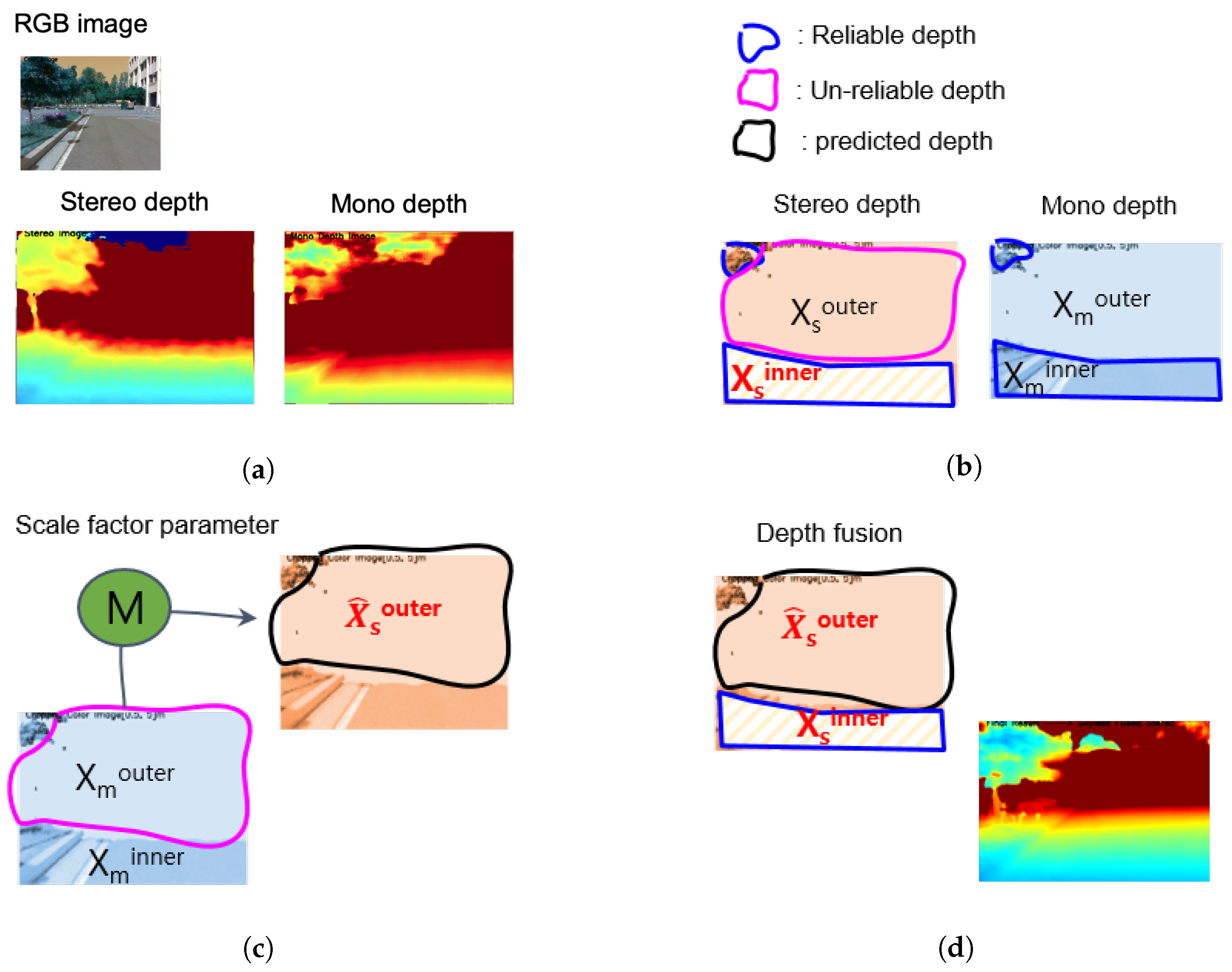
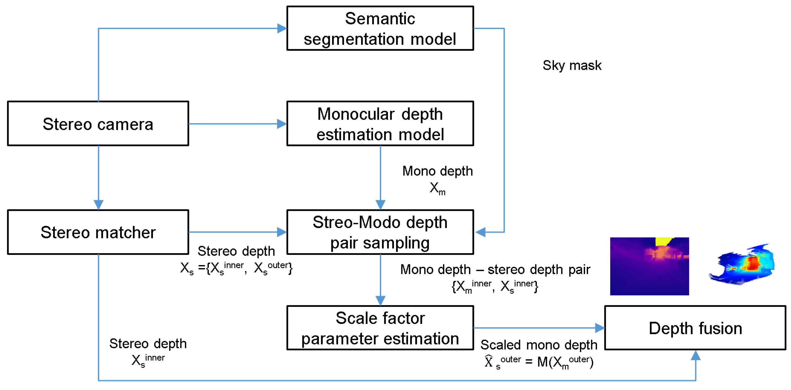
3.1. Overview
- The SD depth () is estimated from the stereo camera.
- MD () is estimated using the MDE model.
- SD and MD pairs {, } are sampled in a reliable depth range.
- The scale factor’s parameter (M) is estimated.
- The scale of the MD outside of the reliable depth () is estimated using the scale factor.
- The SD depth and the scale factor-considered MD are combined to create the expanded depth (FD).
3.2. Stereo-Mono Depth Pairing
| Algorithm 1: Stereo-Mono Depth Pairing |
| Input: , , , , Output: P return P |
3.3. Scale Factor Parameter Estimation
| Algorithm 2: Bucketing |
| Input: , , , , fori from 0 to do , end for return |
3.4. Scale Factor Parameter Update
4. Experimental Results
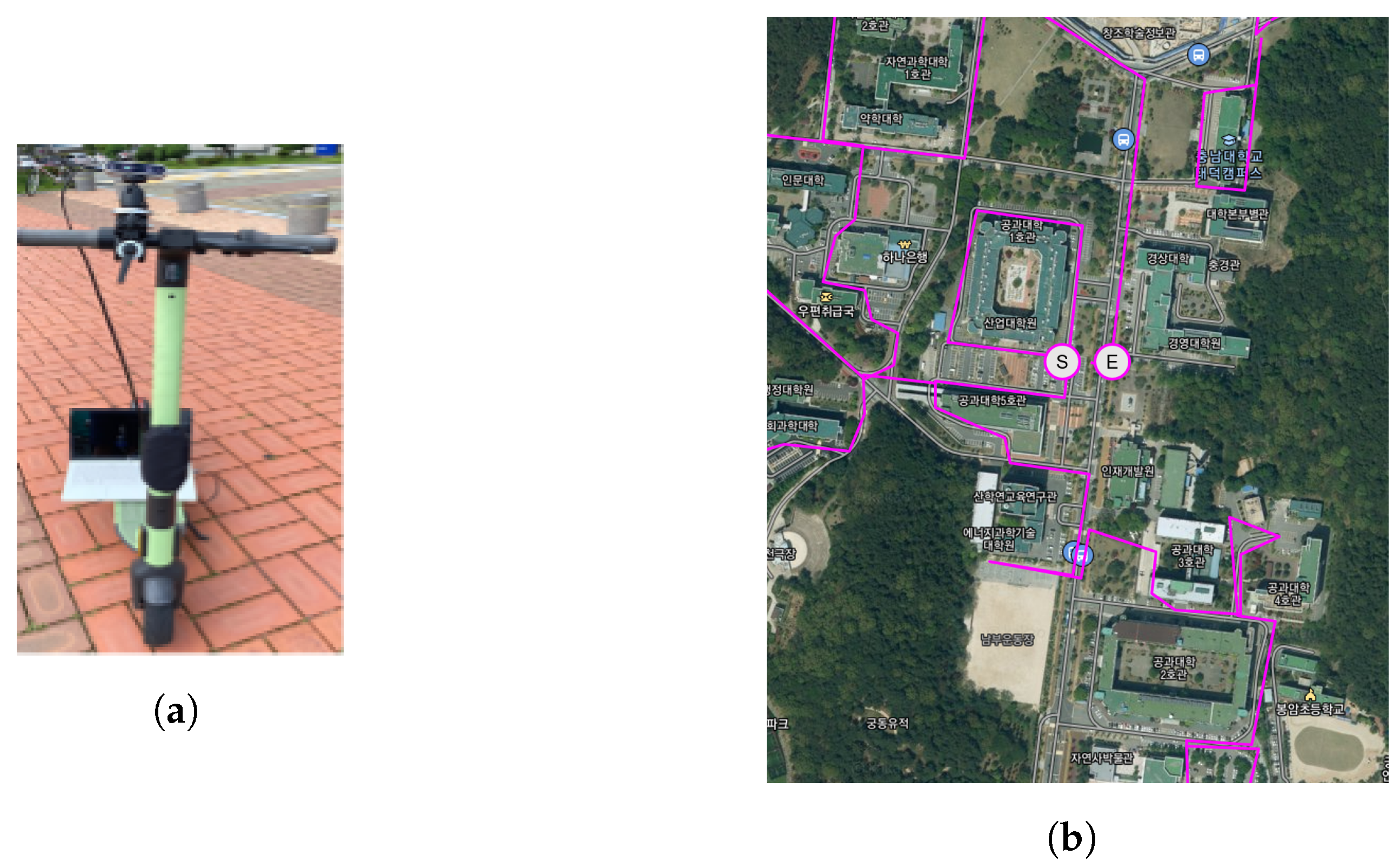
4.1. Datasets and Experimental Setup
4.2. Performance Evaluation
4.3. Computational Performance
5. Conclusions and Future Works
Author Contributions
Funding
Institutional Review Board Statement
Informed Consent Statement
Data Availability Statement
Conflicts of Interest
References
- Kim, J.; Cho, Y.; Kim, A. Exposure Control using Bayesian Optimization based on Entropy Weighted Image Gradient. In Proceedings of the IEEE International Conference on Robotics and Automation, Brisbane, Australia, 21–25 May 2018. [Google Scholar]
- Chang, J.-R.; Chen, Y.-S. Pyramid Stereo Matching Network. In Proceedings of the IEEE Conference on Computer Vision and Pattern Recognition, Salt Lake City, UT, USA, 18–22 January 2018; pp. 5410–5418. [Google Scholar]
- Eigen, D.; Puhrsch, P.; Fergus, R. Depth Map Prediction from a Single Image using a Multi-Scale Deep Network. arXiv 2014, arXiv:1406.2283. [Google Scholar]
- McCraith, R.; Neumann, L.; Vedaldi, A. Calibrating Self-supervised Monocular Depth Estimation. arXiv 2020, arXiv:2009.07714. [Google Scholar]
- Lee, J.H.; Han, M.-K.; Ko, D.W.; Suh, I.H. From big to small: Multi-Scale Local Planar Guidance for Monocular Depth Estimation. arXiv 2019, arXiv:1907.10326. [Google Scholar]
- Song, M.; Lim, S.; Kim, W. Monocular Depth Estimation Using Laplacian Pyramid-Based Depth Residuals. IEEE Trans. Circuits Syst. Video Technol. 2021, 31, 4381–4393. [Google Scholar] [CrossRef]
- Bhat, S.F.; Alhashim, I.; Wonka, P. AdaBins: Depth Estimation Using Adaptive Bins. arXiv 2021, arXiv:2011.14141. [Google Scholar]
- Guizilini, V.; Ambrus, R.; Pillaim, S.; Raventos, A.; Gaidon, A. 3D Packing for Self-Supervised Monocular Depth Estimation. arXiv 2019, arXiv:1905.02693. [Google Scholar]
- Li, Z.; Wang, X.; Liu, X.; Jiang, J. BinsFormer: Revisiting Adaptive Bins for Monocular Depth Estimation. arXiv 2022, arXiv:2204.00987. [Google Scholar]
- Li, Z.; Wang, X.; Liu, X.; Jiang, J. DepthFormer: Exploiting Long-Range Correlation and Local Information for Accurate Monocular Depth Estimation. arXiv 2022, arXiv:2203.14211. [Google Scholar]
- Ranftl, R.; Bochkovskiy, A.; Koltun, V. Vision Transformers for Dense Prediction. arXiv 2021, arXiv:2103.13413. [Google Scholar]
- Geiger, A.; Lenz, P.; Stiller, C.; Urtasun, R. Vision Meets Robotics: The Kitti Dataset. Int. J. Rob. Res. 2013, 32, 1231–1237. [Google Scholar] [CrossRef] [Green Version]
- Bauer, Z.; Gomez-Donoso, F.; Cruz, E.; Orts-Escolano, S.; Cazorla, M. UASOL, A Large-Scale High-Resolution Outdoor Stereo Dataset. Sci. Data 2019, 6, 162. [Google Scholar] [CrossRef] [PubMed] [Green Version]
- Sheeny, M.; Pellegrin, E.D.; Saptarshi, M.; Ahrabian, A.; Wang, S.; Wallace, A. RADIATE: A Radar Dataset for Automotive Perception. arXiv 2020, arXiv:2010.09076. [Google Scholar]
- Ahn, M.S.; Chae, H.; Noh, D.; Nam, H.; Hong, D. Analysis and Noise Modeling of the Intel RealSense D435 for Mobile Robots. In Proceedings of the International Conference on Ubiquitous Robots, Jeju, Korea, 24–27 June 2019. [Google Scholar]
- Halmetschlager-Funek, G.; Suchi, M.; Kampel, M.; Vincze, M. An Empirical Evaluation of Ten Depth Cameras: Bias, Precision, Lateral Noise, Different Lighting Conditions and Materials, and Multiple Sensor Setups in Indoor Environments. IEEE Robot. Autom. Mag. 2019, 26, 67–77. [Google Scholar] [CrossRef]
- Chen, L.-C.; Papandreou, G.; Schroff, F.; Adam, H. Rethinking Atrous Convolution for Semantic Image Segmentation. arXiv 2017, arXiv:1706.05587. [Google Scholar]
- Cordts, M.; Omran, M.; Ramos, S.; Rehfeld, T.; Enzweiler, M.; Benenson, R.; Franke, U.; Roth, S.; Schiele, B. The Cityscapes Dataset for Semantic Urban Scene Understanding. In Proceedings of the IEEE Conference on Computer Vision and Pattern Recognition, Las Vegas, NV, USA, 26 June–1 July 2017. [Google Scholar]
- Howard, A.G.; Zhu, M.; Chen, B.; Kalenichenko, D.; Wang, W.; Weyand, T.; Andreetto, M.; Adam, H. MobileNets: Efficient Convolutional Neural Networks for Mobile Vision Applications. arXiv 2016, arXiv:1704.04861. [Google Scholar]
- Wofk, D.; Ma, F.; Yang, T.J.; Karaman, S.; Sze, V. Fastdepth: Fast monocular depth estimation on embedded systems. In Proceedings of the 2019 International Conference on Robotics and Automation (ICRA), Montreal, QC, Canada, 20–24 May 2019; pp. 6101–6108. [Google Scholar]


| Errors | Equations |
|---|---|
| Average relative error (AR) | |
| Squared relative difference (SR) | |
| Root mean squared error (RS) | |
| Average Log 10 error (L10) |
| DB | Network | GT vs. | Evaluation Results | |||||||||||
|---|---|---|---|---|---|---|---|---|---|---|---|---|---|---|
| AR | SR | RS | L10 | |||||||||||
| D10 1 | D15 2 | D20 3 | D10 | D15 | D20 | D10 | D15 | D20 | D10 | D15 | D20 | |||
| UASOL | BTS | MD | 0.35 | 0.45 | 0.56 | 1.39 | 4.54 | 7.66 | 2.97 | 6.64 | 10.49 | 0.17 | 0.25 | 0.29 |
| FD | 0.14 | 0.33 | 0.47 | 0.32 | 2.31 | 5.61 | 1.31 | 4.67 | 8.76 | 0.05 | 0.16 | 0.26 | ||
| AdaBins | MD | 0.30 | 0.43 | 0.47 | 1.11 | 3.02 | 4.91 | 2.57 | 5.74 | 8.78 | 0.12 | 0.21 | 0.26 | |
| FD | 0.13 | 0.32 | 0.44 | 0.31 | 1.82 | 4.28 | 1.26 | 4.40 | 8.04 | 0.04 | 0.16 | 0.24 | ||
| RADIATE | BTS | MD | 0.56 | 0.59 | 0.55 | 2.76 | 5.50 | 7.35 | 4.45 | 8.25 | 11.01 | 0.19 | 0.19 | 0.17 |
| FD | 0.09 | 0.19 | 0.27 | 0.12 | 0.68 | 1.68 | 0.89 | 2.89 | 5.19 | 0.03 | 0.08 | 0.12 | ||
| AdaBins | MD | 0.44 | 0.506 | 0.46 | 1.88 | 4.06 | 4.92 | 3.64 | 7.04 | 8.99 | 0.16 | 0.16 | 0.13 | |
| FD | 0.1 | 0.14 | 0.21 | 0.16 | 0.53 | 1.27 | 1.01 | 2.50 | 4.56 | 0.022 | 0.04 | 0.07 | ||
| DB | Network | ST vs. | Evaluation Metrics | |||
|---|---|---|---|---|---|---|
| AR (D10) 2 | SR (D10) | RS: (D10) | L10 (D01) | |||
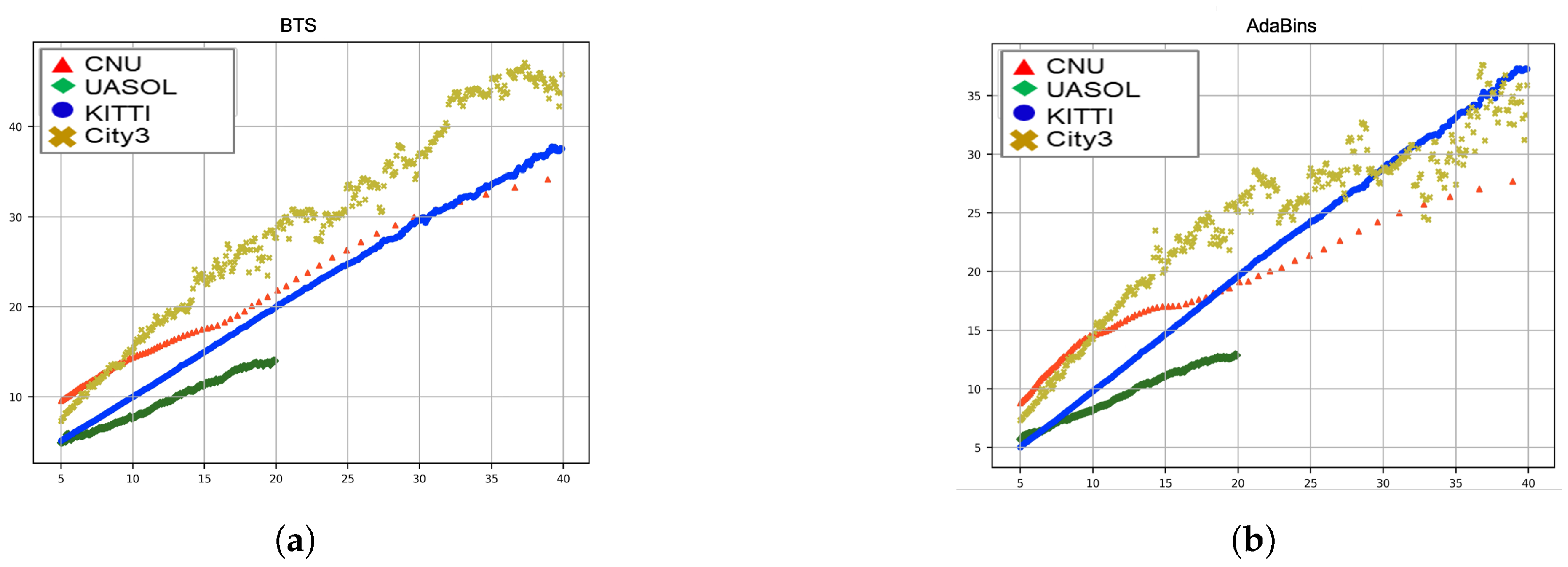
| CNU | BTS | MD | 0.653 | 3.85 | 5.186 | 0.206 |
| FD | 0.153 | 0.37 | 1.481 | 0.043 | ||
| AdaBins | MD | 0.653 | 4.106 | 5.302 | 0.202 | |
| FD | 0.147 | 0.294 | 1.013 | 0.042 | ||
| Network | Measure | CNU (640 × 480) | UASOL (1216 × 352) | RADIATE (640 × 480) | KITTI (1216 × 352) |
|---|---|---|---|---|---|
| BTS | # of SFPE 1/sample | 4/1760 | 74/205 | 7/719 | 0/433 |
| SFPE time (/) (s) | 0.014/0.004 | 0.061/0.055 | 0.013/0.009 | 0.020/0.004 | |
| MDE time (/) (s) | 0.159/0.004 | 0.432/0.010 | 0.160/0.007 | 0.215/0.007 | |
| Total (s) | 0.173 | 0.493 | 0.173 | 0.235 | |
| AdaBins | # of SFPE/sample | 9/1760 | 66/205 | 0/719 | 0/433 |
| SFPE time (/) (s) | 0.014/0.005 | 0.057/0.057 | 0.012/0.003 | 0.019/0004 | |
| MDE time (/) (s) | 0.201/0.002 | 0.230/0.004 | 0.203/0.002 | 0.227/0.002 | |
| Total time (s) | 0.215 | 0.287 | 0.215 | 0.246 |
| Depth Methods | Pros | Cons |
|---|---|---|
| LiDAR | accurate | sparse, high cost and energy, relatively more mounting space |
| Stereo 1 | dense, relatively low cost and energy, less mounting space | accurate only within short distance 3 |
| Monocular 2 | same with stereo depth | require data manipulation 4 and retraining of CNNs if not like with train environments |
| Proposed Method | same with stereo depth, no manipulation, and retraining | relatively inaccurate if used in the train environments compared with MDE |
Publisher’s Note: MDPI stays neutral with regard to jurisdictional claims in published maps and institutional affiliations. |
© 2022 by the authors. Licensee MDPI, Basel, Switzerland. This article is an open access article distributed under the terms and conditions of the Creative Commons Attribution (CC BY) license (https://creativecommons.org/licenses/by/4.0/).
Share and Cite
Seo, B.-S.; Park, B.; Choi, H. Sensing Range Extension for Short-Baseline Stereo Camera Using Monocular Depth Estimation. Sensors 2022, 22, 4605. https://doi.org/10.3390/s22124605
Seo B-S, Park B, Choi H. Sensing Range Extension for Short-Baseline Stereo Camera Using Monocular Depth Estimation. Sensors. 2022; 22(12):4605. https://doi.org/10.3390/s22124605
Chicago/Turabian StyleSeo, Beom-Su, Byungjae Park, and Hoon Choi. 2022. "Sensing Range Extension for Short-Baseline Stereo Camera Using Monocular Depth Estimation" Sensors 22, no. 12: 4605. https://doi.org/10.3390/s22124605
APA StyleSeo, B.-S., Park, B., & Choi, H. (2022). Sensing Range Extension for Short-Baseline Stereo Camera Using Monocular Depth Estimation. Sensors, 22(12), 4605. https://doi.org/10.3390/s22124605