
Classification of Plank Techniques Using Wearable Sensors


Abstract
:1. Introduction
2. Materials and Methods
2.1. Subjects
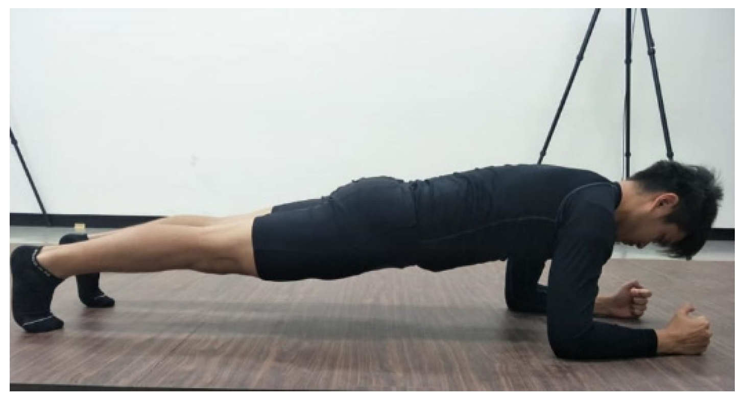
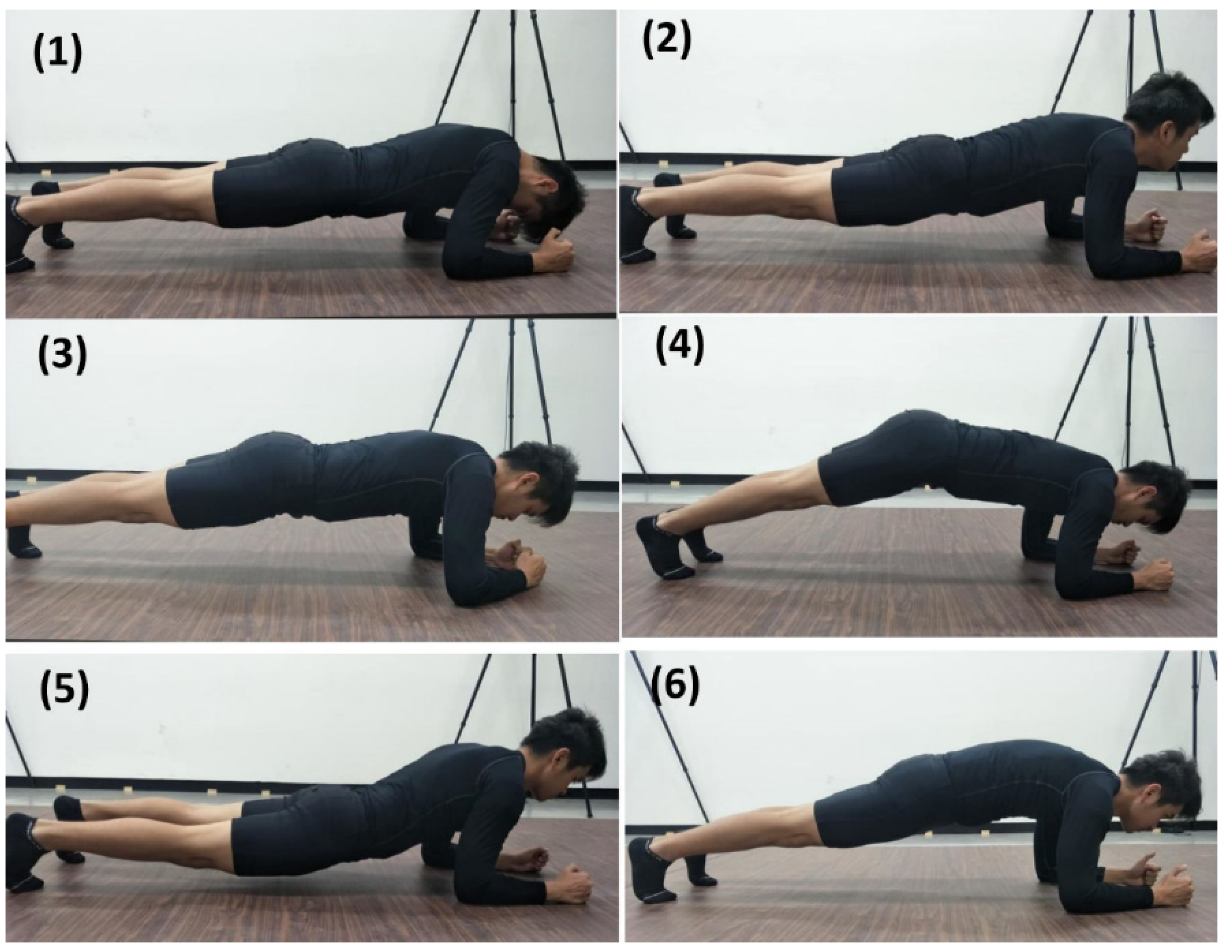
2.2. Procedures
2.3. Data Collection
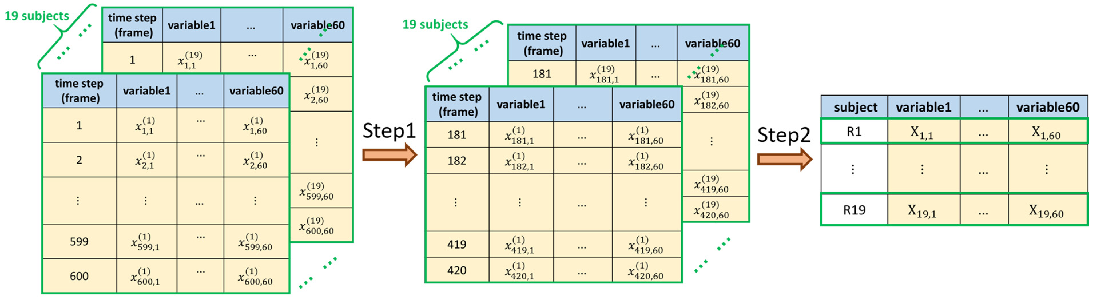
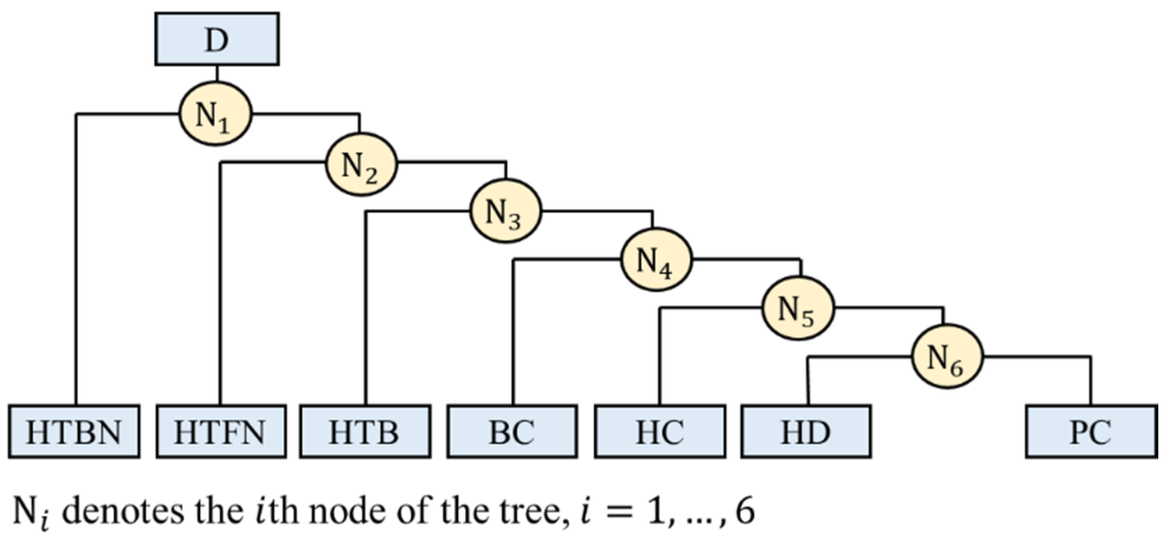
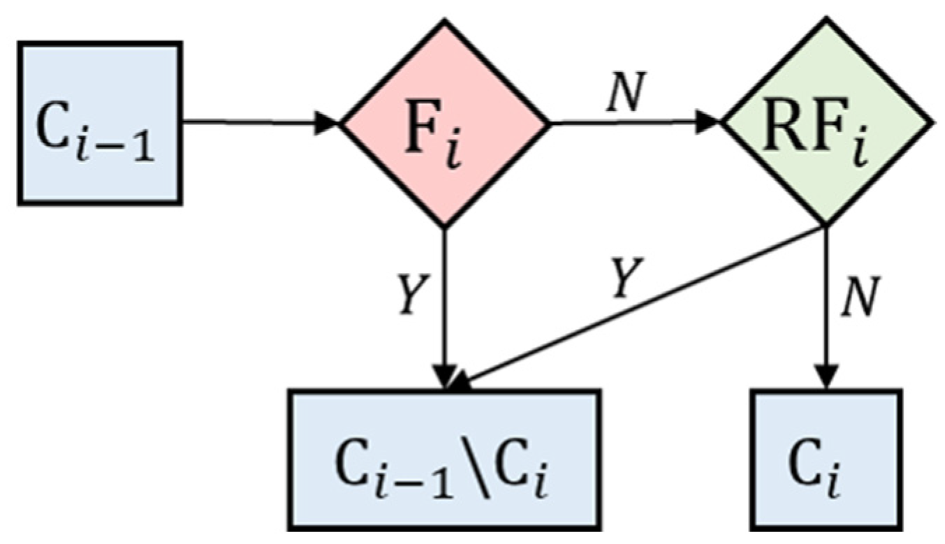
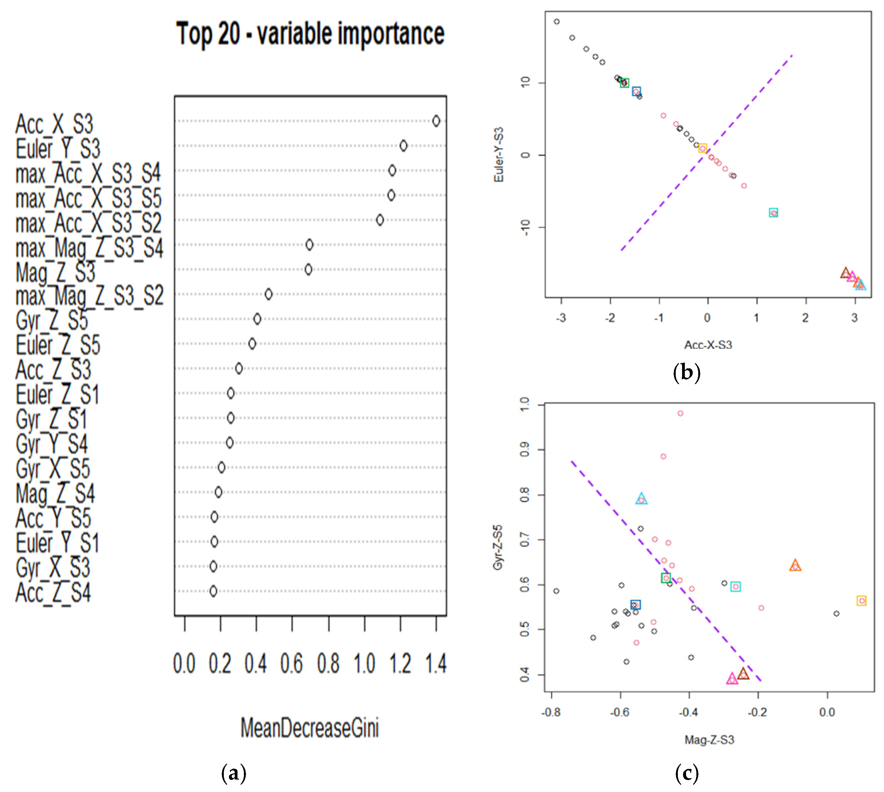
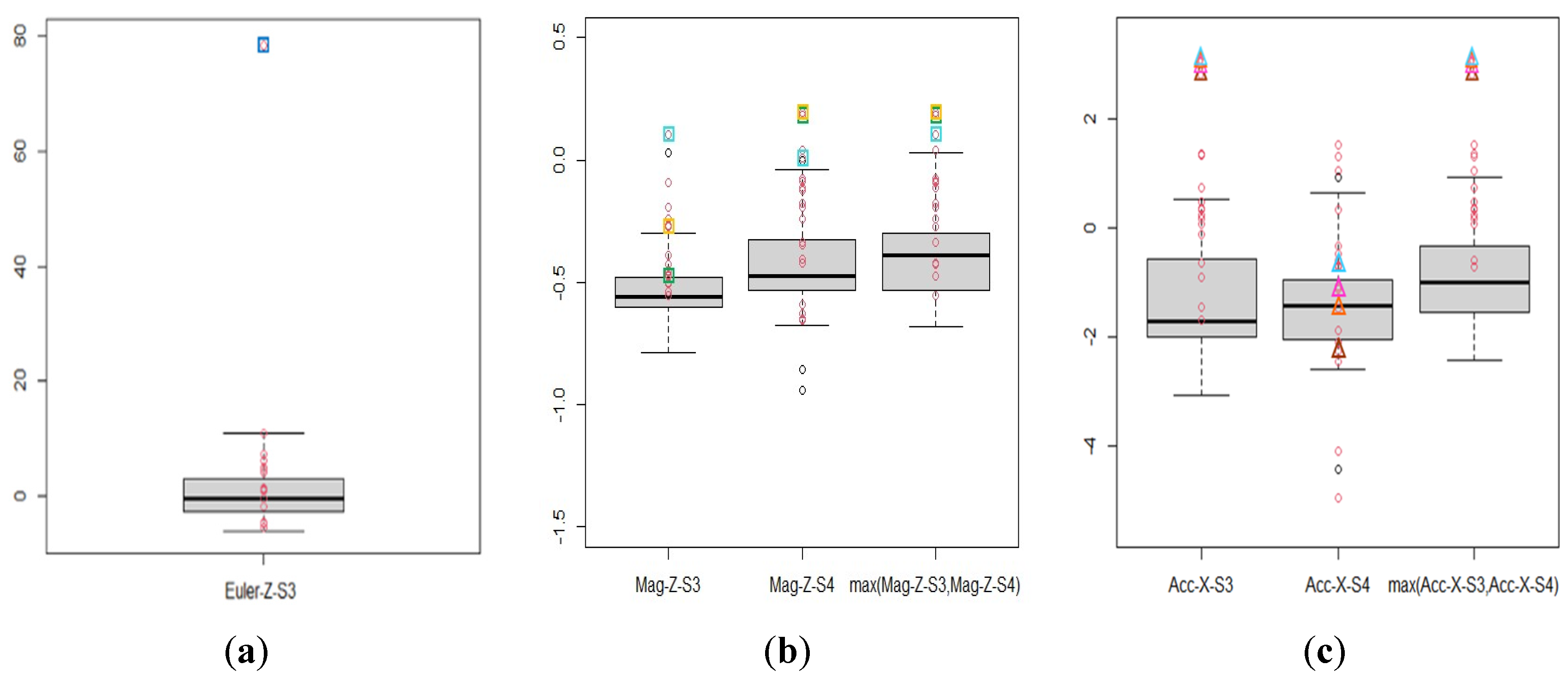
2.4. Data Analysis
- For a fixed filtered variable in each replication, we used the values in set of the training data to establish an empirical distribution.
- For each observation in the test set, we computed the p-value of the filtered variable based on the empirical distribution above.
3. Results
4. Discussion
5. Conclusions
Author Contributions
Funding
Institutional Review Board Statement
Informed Consent Statement
Data Availability Statement
Acknowledgments
Conflicts of Interest
References
- Adesida, Y.; Papi, E.; McGregor, A.H. Exploring the role of wearable technology in sport kinematics and kinetics: A systematic review. Sensors 2019, 19, 1597. [Google Scholar] [CrossRef] [Green Version]
- Camomilla, V.; Bergamini, E.; Fantozzi, S.; Vannozzi, G. Trends supporting the in-field use of wearable inertial sensors for sport performance evaluation: A systematic review. Sensors 2018, 18, 873. [Google Scholar]
- O’Reilly, M.A.; Caulfield, B.; Ward, T.; Johnston, W.; Doherty, C. Wearable inertial sensor systems for lower limb exercise detection and evaluation: A systematic review. Sports Med. 2018, 48, 1221–1246. [Google Scholar] [CrossRef] [Green Version]
- O’Reilly, M.A.; Whelan, D.F.; Ward, T.E.; Delahunt, E.; Caulfield, B.M. Technology in strength and conditioning: Assessing bodyweight squat technique with wearable sensors. J. Strength Cond. Res. 2017, 31, 2303–2312. [Google Scholar] [CrossRef]
- O’Reilly, M.A.; Whelan, D.F.; Ward, T.E.; Delahunt, E.; Caulfield, B. Classification of lunge biomechanics with multiple and individual inertial measurement units. Sports Biomech. 2017, 16, 342–360. [Google Scholar]
- Giggins, O.M.; Sweeney, K.T.; Caulfield, B. Rehabilitation exercise assessment using inertial sensors: A cross-sectional analytical study. J. Neuroeng. Rehabil. 2014, 11, 158–168. [Google Scholar] [CrossRef] [Green Version]
- Whelan, D.F.; O’Reilly, M.A.; Ward, T.E.; Delahunt, E.; Caulfield, B. Technology in rehabilitation: Evaluating the single leg squat exercise with wearable inertial measurement units. Methods Inf. Med. 2017, 56, 88–94. [Google Scholar]
- Wang, Q.; Markopoulos, P.; Yu, B.; Chen, W.; Timmermans, A. Interactive wearable systems for upper body rehabilitation: A systematic review. J. Neuroeng. Rehabil. 2017, 14, 20. [Google Scholar] [CrossRef] [Green Version]
- Johnston, W.; O’Reilly, M.A.; Argent, R.; Caulfield, B. Reliability, validity and utility of inertial sensor systems for postural control assessment in sport science and medicine applications: A systematic review. Sports Med. 2019, 49, 783–818. [Google Scholar] [CrossRef] [Green Version]
- Kibler, W.B.; Press, J.; Sciascia, A. The role of core stability in athletic function. Sports Med. 2006, 36, 189–198. [Google Scholar] [CrossRef]
- Willardson, J.M. Core stability training: Applications to sports conditioning programs. J. Strength Cond. Res. 2007, 21, 979–985. [Google Scholar] [CrossRef]
- Frizziero, A.; Pellizzon, G.; Vittadini, F.; Bigliardi, D.; Costantino, C. Efficacy of core stability in non-specific chronic low back pain. J. Funct. Morphol. Kinesiol. 2021, 6, 37. [Google Scholar] [CrossRef]
- Ekstrom, R.A.; Donatelli, R.A.; Carp, K.C. Electromyographic analysis of core trunk, hip, and thigh muscles during 9 rehabilitation exercises. J. Orthop. Sports Phys. Ther. 2007, 37, 754–762. [Google Scholar] [CrossRef] [Green Version]
- Snarr, R.L.; Esco, M.R. Electromyographical comparison of plank variations performed with and without instability devices. J. Strength Cond. Res. 2014, 28, 3298–3305. [Google Scholar] [CrossRef]
- Tong, T.K.; Wu, S.; Nie, J. Sport-specific endurance plank test for evaluation of global core muscle function. Phys. Ther. Sport 2014, 15, 58–63. [Google Scholar] [CrossRef]
- Strand, S.L.; Hjelm, J.; Shoepe, T.C.; Fajardo, M.A. Norms for an isometric muscle endurance test. J. Hum. Kinet. 2014, 40, 93–102. [Google Scholar] [CrossRef] [Green Version]
- Bös, K.; Brehm, W.; Klemm, K.; Schreck, M.; Pauly, P. European Fitness Badge: Handbook for Instructors; Deutscher Turner-Bund eV (DTB): Frankfurt, Germany, 2017. [Google Scholar]
- Ross, G.B.; Dowling, B.; Troje, N.F.; Fischer, S.L.; Graham, R.B. Objectively differentiating movement patterns between elite and novice athletes. Med. Sci. Sports Exerc. 2018, 50, 1457–1464. [Google Scholar] [CrossRef]
- NSCA—National Strength & Conditioning Association. Developing the Core; Human Kinetics: Champaign, IL, USA, 2014. [Google Scholar]
- Breiman, L. Random forests. Mach. Learn. 2001, 45, 5–32. [Google Scholar] [CrossRef] [Green Version]
- Ahmad, I.; Basheri, M.; Iqbal, M.J.; Rahim, A. Performance comparison of support vector machine, random forest, and extreme learning machine for intrusion detection. IEEE Access 2018, 6, 33789–33795. [Google Scholar] [CrossRef]
- Jonathan, B.; Sihotang, J.I.; Martin, S. Sentiment Analysis of Customer Reviews in Zomato Bangalore Restaurants Using Random Forest Classifier. In Proceedings of the 7th International Scholars Conference, Jawa Barat, Indonesia, 28–29 October 2019; pp. 1719–1728. [Google Scholar]
- Huang, S.F.; Wen, Y.H.; Chu, C.H.; Hsu, C.C. A shape approximation for medical imaging data. Sensors 2020, 20, 5879. [Google Scholar] [CrossRef]
- Huang, S.F.; Guo, M.; Chen, M.R. Stock market trend prediction using a functional time series approach. Quant. Financ. 2020, 20, 69–79. [Google Scholar] [CrossRef]
- Huang, S.F.; Lin, Y.W. A feature fusion approach for multiple signal classification. In Proceedings of the 2020 International Computer Symposium, Tainan, Taiwan, 17–19 December 2020; pp. 37–42. [Google Scholar]
- Yoon, C.; Lee, J.; Kim, K.; Kim, H.C.; Chung, S.G. Quantification of lumbar stability during wall plank-and-roll activity using inertial sensors. PM R 2015, 7, 803–813. [Google Scholar] [CrossRef]
- Panjabi, M.M. The stabilizing system of the spine. Part II. Neutral zone and instability hypothesis. J. Spinal Disord. 1992, 5, 390–396. [Google Scholar] [CrossRef]
- Cortell-Tormo, J.M.; García-Jaén, M.; Chulvi-Medrano, I.; Hernández-Sánchez, S.; Lucas-Cuevas, Á.G.; Tortosa-Martínez, J. Influence of scapular position on the core musculature activation in the prone plank exercise. J. Strength Cond. Res. 2017, 31, 2255–2262. [Google Scholar] [CrossRef]


| Training Set | ||||
|---|---|---|---|---|
| Accuracy | ||||
| HTBN | 15 | 90 | 100% (0.00) | |
| HTFN | 15 | 75 | 100% (0.00) | |
| HTB | 15 | 60 | 100% (0.00) | |
| BC | 15 | 45 | 100% (0.00) | |
| HC | 15 | 30 | 100% (0.00) | |
| HD | 15 | 15 | 100% (0.00) | |
| Test Set | ||||||
|---|---|---|---|---|---|---|
| Accuracy | Sensitivity | Specificity | ||||
| HTBN | 4 | 24 | 100% (0.00) | 100% (0.00) | 100% (0.00) | |
| HTFN | 4 | 20 | 97% (0.02) | 91% (0.13) | 98% (0.03) | |
| HTB | 4 | 16 | 93% (0.06) | 92% (0.14) | 93% (0.07) | |
| BC | 4 | 12 | 91% (0.08) | 92% (0.12) | 91% (0.09) | |
| HC | 4 | 8 | 93% (0.06) | 94% (0.12) | 93% (0.09) | |
| HD | 4 | 4 | 86% (0.11) | 90% (0.15) | 83% (0.19) | |
| Gyr-Z-S3 | Euler-Z-S3 | max(Euler-Z-S5, Euler-Z-S1) | Euler-Z-S3 |
| Acc-X-S4 | max(Euler-Z-S5, Euler-Z-S2) | max(Acc-X-S3, Acc-X-S2) | |
| max(Euler-Z-S5, Euler-Z-S3) | max(Acc-X-S3, Acc-X-S4) | ||
| max(Euler-Z-S5, Euler-Z-S4) | max(Acc-X-S3, Acc-X-S5) | ||
| max(Mag-Z-S3, Mag-Z-S2) | |||
| max(Mag-Z-S3, Mag-Z-S4) |
Publisher’s Note: MDPI stays neutral with regard to jurisdictional claims in published maps and institutional affiliations. |
© 2022 by the authors. Licensee MDPI, Basel, Switzerland. This article is an open access article distributed under the terms and conditions of the Creative Commons Attribution (CC BY) license (https://creativecommons.org/licenses/by/4.0/).
Share and Cite
Chen, Z.-R.; Tsai, W.-C.; Huang, S.-F.; Li, T.-Y.; Song, C.-Y. Classification of Plank Techniques Using Wearable Sensors. Sensors 2022, 22, 4510. https://doi.org/10.3390/s22124510
Chen Z-R, Tsai W-C, Huang S-F, Li T-Y, Song C-Y. Classification of Plank Techniques Using Wearable Sensors. Sensors. 2022; 22(12):4510. https://doi.org/10.3390/s22124510
Chicago/Turabian StyleChen, Zong-Rong, Wei-Chi Tsai, Shih-Feng Huang, Tzu-Yi Li, and Chen-Yi Song. 2022. "Classification of Plank Techniques Using Wearable Sensors" Sensors 22, no. 12: 4510. https://doi.org/10.3390/s22124510
APA StyleChen, Z.-R., Tsai, W.-C., Huang, S.-F., Li, T.-Y., & Song, C.-Y. (2022). Classification of Plank Techniques Using Wearable Sensors. Sensors, 22(12), 4510. https://doi.org/10.3390/s22124510