
RT-ViT: Real-Time Monocular Depth Estimation Using Lightweight Vision Transformers


Abstract
:1. Introduction
- We propose efficient architectures for accurate depth estimation based on a ViT encoder and convolutional decoder architectures;
- We show that the proposed model can attain a high speed of frame processing (∼20 fps) which is convenient for real-time depth estimation;
- We propose architectures with different combinations composed of four ViT-based encoder architectures and four different CNN-based decoder architectures;
- We show that the ViT encoder can extract much more representative features and so a better depth estimation accuracy than the fully convolutional-based architectures and even some ViT-based architectures by comparison.
2. Related Work
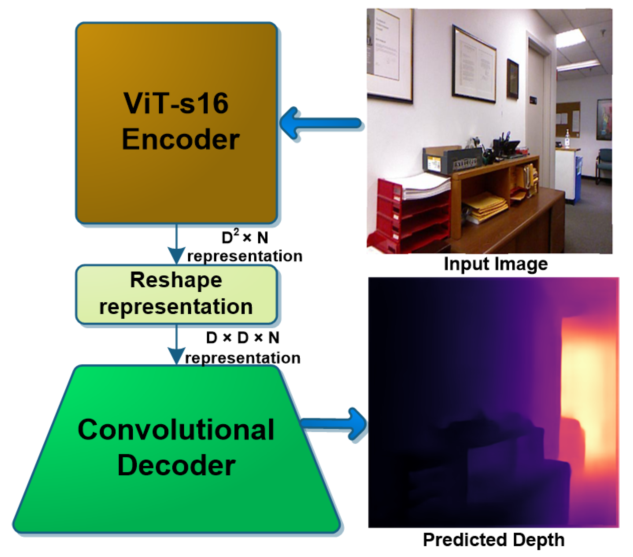
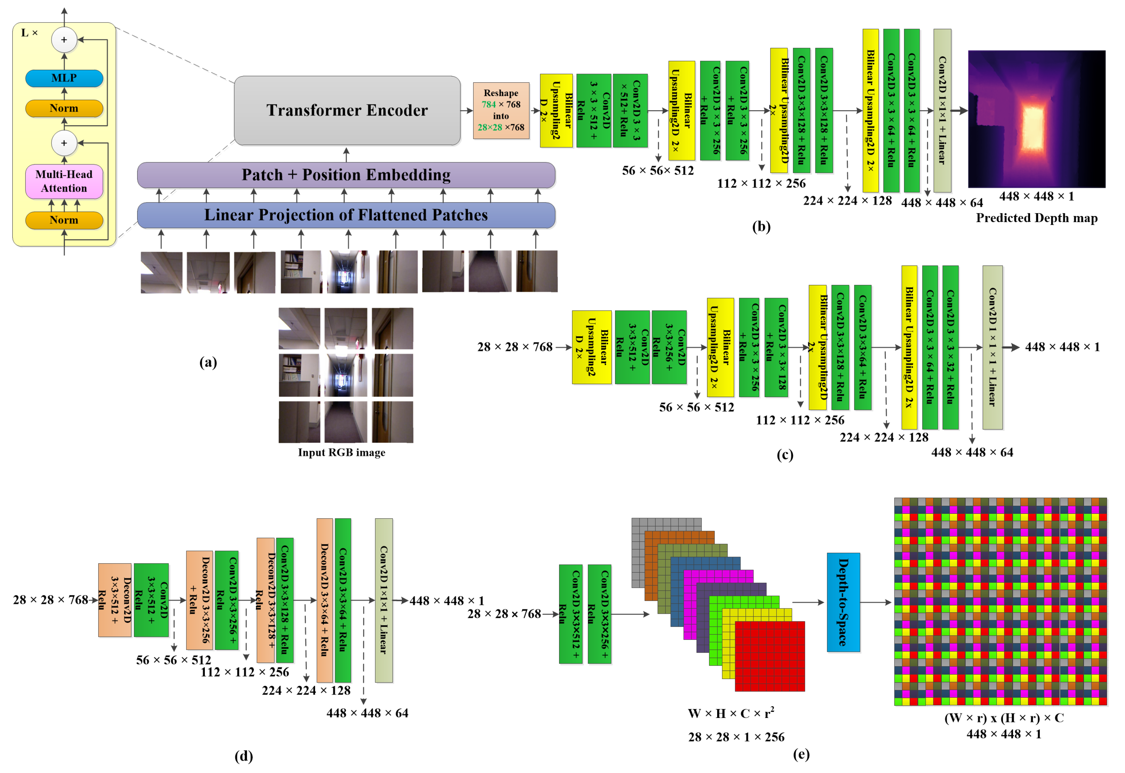
3. Proposed Method
3.1. ViT Encoder Architectures
3.2. CNN Decoder Architectures
4. Benchmarks for Training and Validation
5. Experiments
6. Evaluation Metrics
- The delta accuracy of : for threshold values ;
- The absolute relative error (Abs_Rel): ;
- The squared relative error (Sq_Rel): ;
- The root mean squared error (): ,
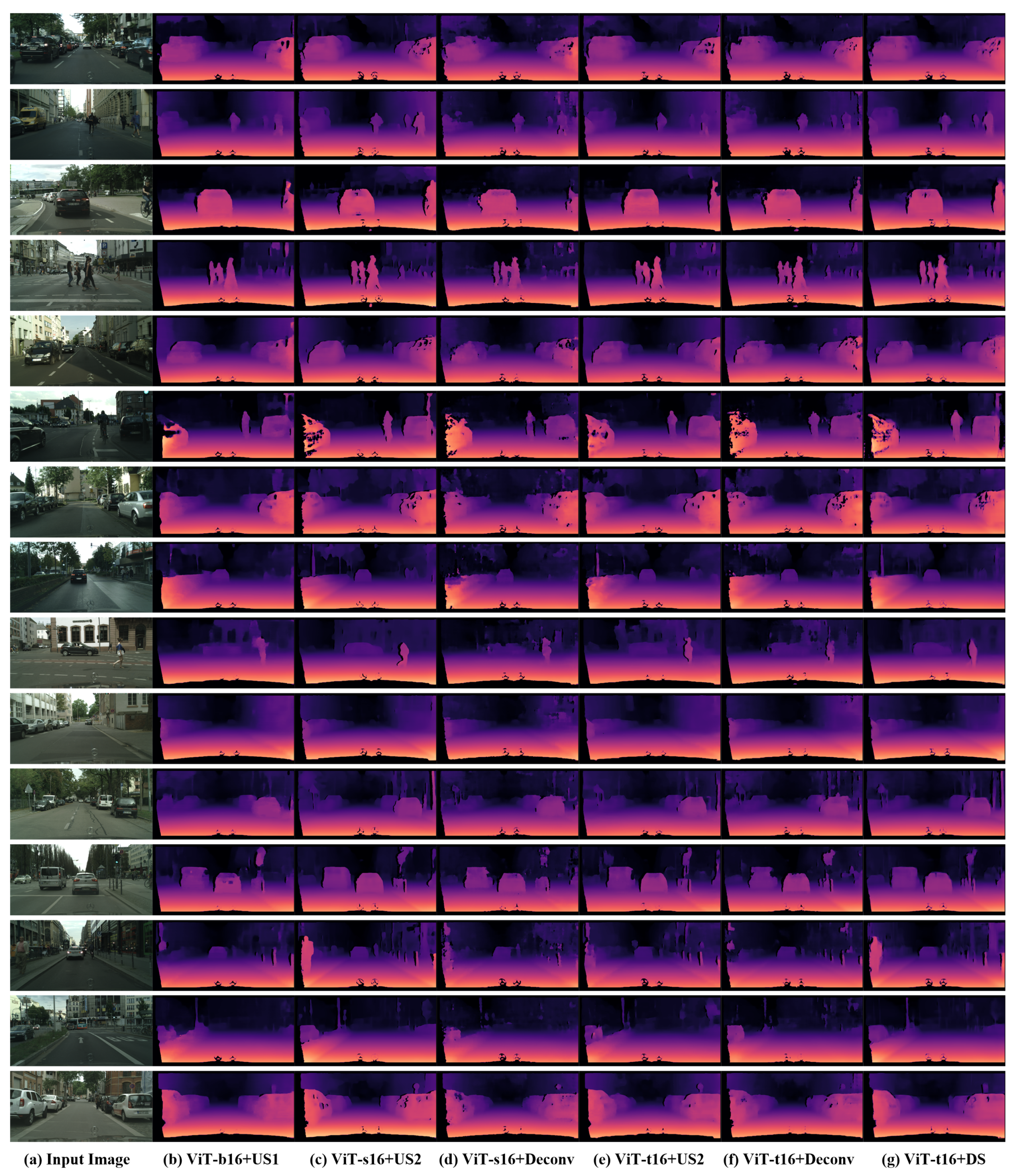
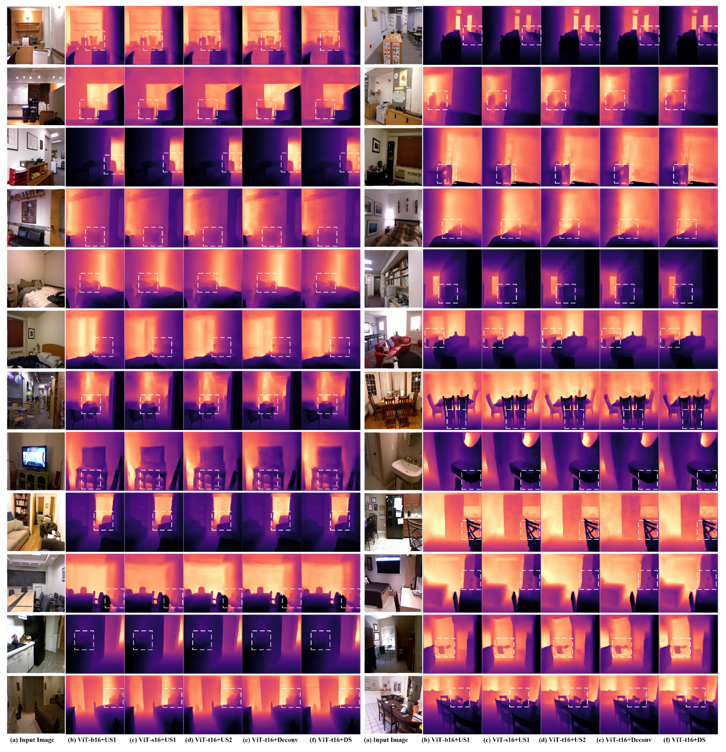
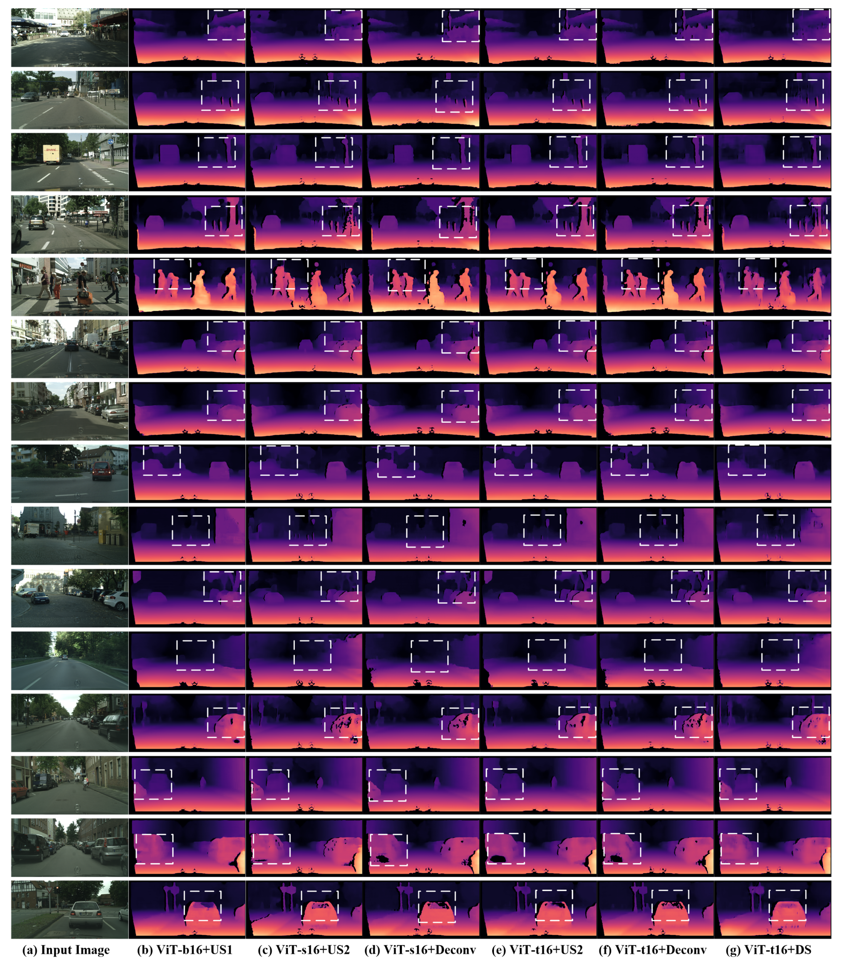
7. Results
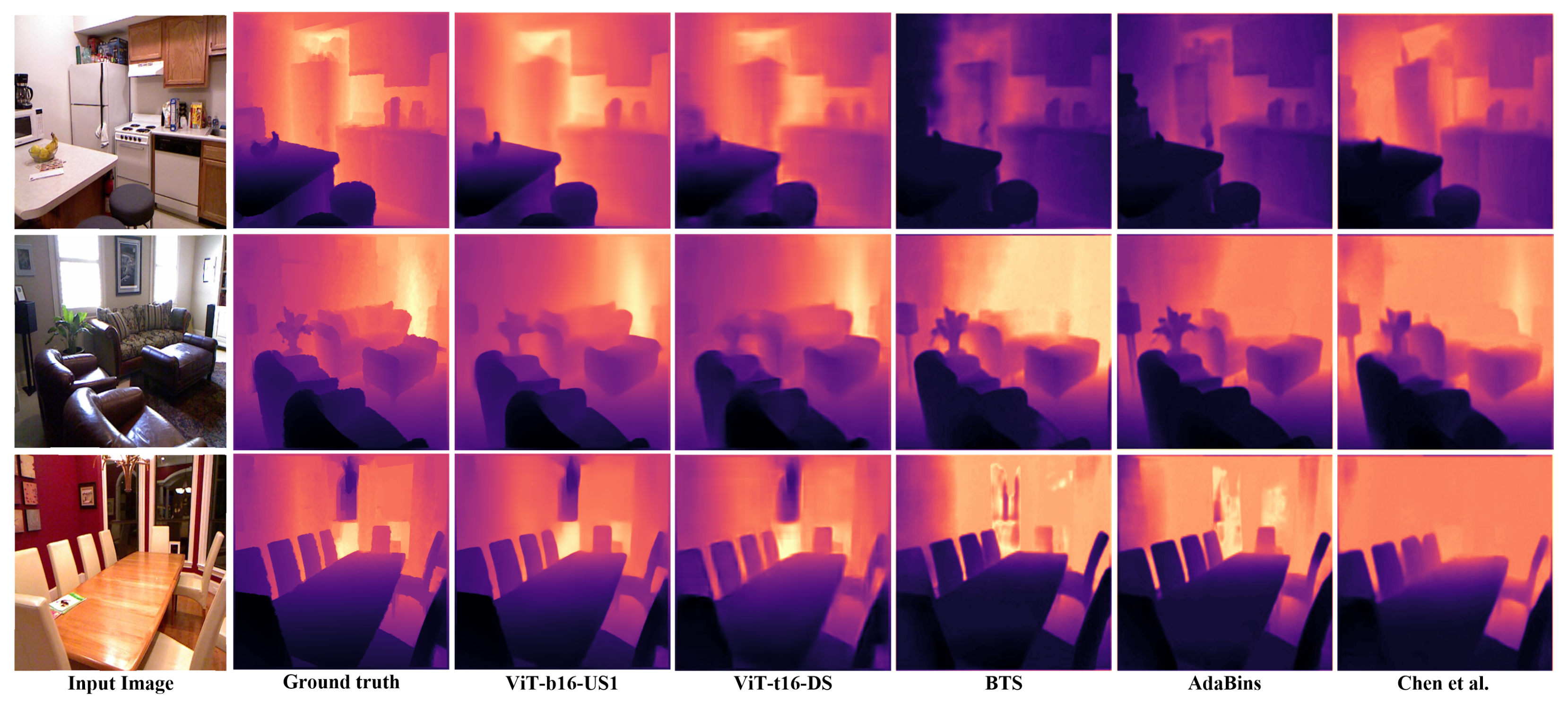
8. Comparison with the SOTA Methods
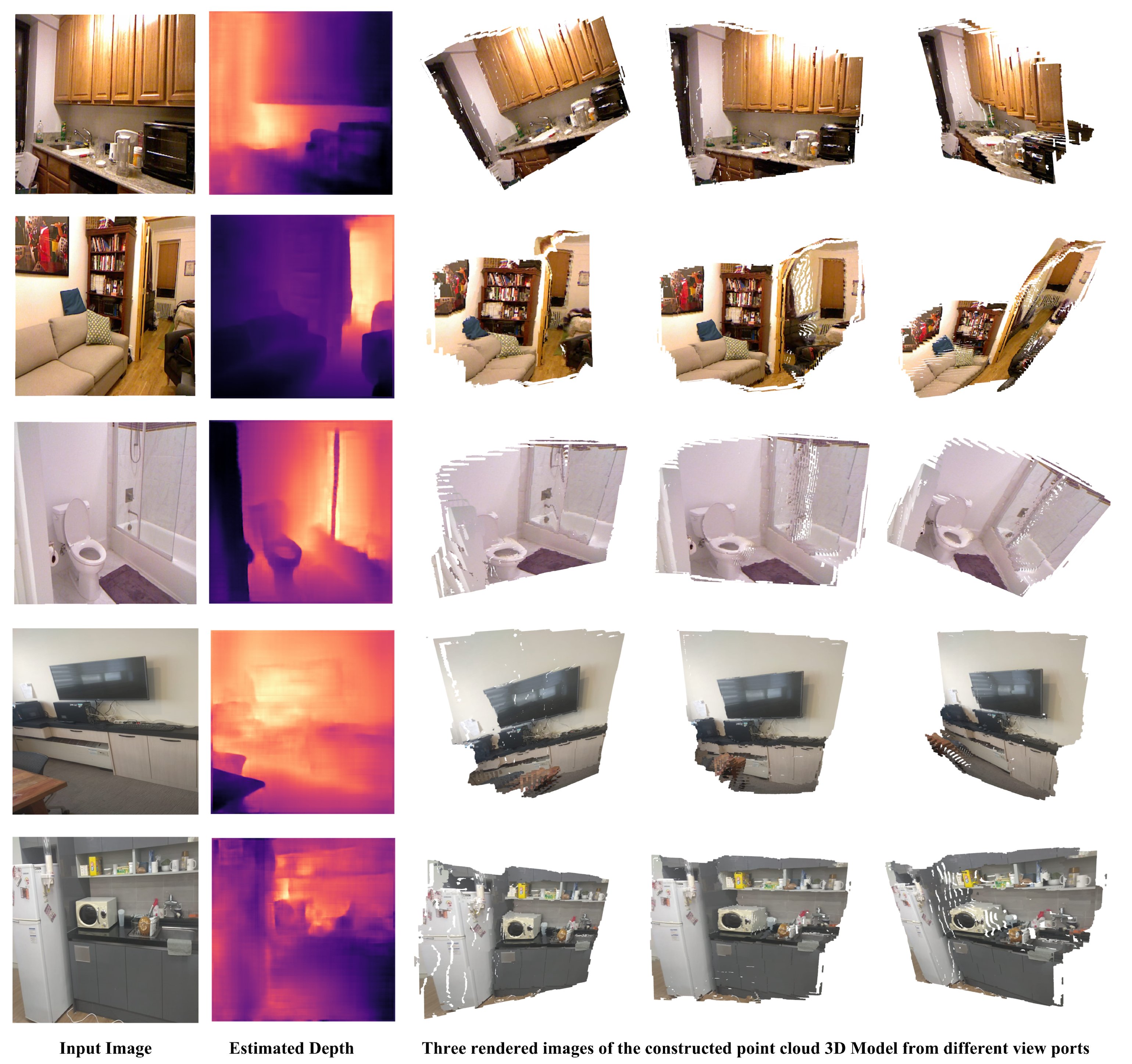
9. Fast 3D Reconstruction as an Application of the Proposed Method
10. Conclusions
11. Future Work
Author Contributions
Funding
Institutional Review Board Statement
Informed Consent Statement
Data Availability Statement
Conflicts of Interest
Appendix A
References
- Eigen, D.; Puhrsch, C.; Fergus, R. Depth Map Prediction from a Single Image using a Multi-Scale Deep Network. In Proceedings of the Advances in Neural Information Processing Systems (NeurIPs), Montréal, QC, Canada, 8–13 December 2014. [Google Scholar]
- Li, J.; Klein, R.; Yao, A. A Two-Streamed Network for Estimating Fine-Scaled Depth Maps from Single RGB Images. In Proceedings of the IEEE International Conference on Computer Vision (ICCV), Venice, Italy, 22–29 October 2017; pp. 3392–3400. [Google Scholar]
- Liu, F.; Shen, C.; Lin, G. Deep convolutional neural fields for depth estimation from a single image. In Proceedings of the IEEE Conference on Computer Vision and Pattern Recognition (CVPR), Boston, MA, USA, 7–12 June 2015; pp. 5162–5170. [Google Scholar]
- Gan, Y.; Xu, X.; Sun, W.; Lin, L. Monocular Depth Estimation with Affinity, Vertical Pooling, and Label Enhancement. In Proceedings of the IEEE European Conference on Computer Vision (ECCV), Munich, Germany, 8–14 September 2018; pp. 224–239. [Google Scholar]
- Xu, D.; Ricci, E.; Ouyang, W.; Wang, X.; Sebe, N. Multi-scale Continuous CRFs as Sequential Deep Networks for Monocular Depth Estimation. In Proceedings of the IEEE Conference on Computer Vision and Pattern Recognition (CVPR), Honolulu, HI, USA, 21–26 July 2017; pp. 161–169. [Google Scholar]
- Kuznietsov, Y.; Stückler, J.; Leibe, B. Semi-Supervised Deep Learning for Monocular Depth Map Prediction. In Proceedings of the IEEE Conference on Computer Vision and Pattern Recognition (CVPR), Honolulu, HI, USA, 21–26 July 2017; pp. 2215–2223. [Google Scholar]
- Fu, H.; Gong, M.; Wang, C.; Batmanghelich, K.; Tao, D. Deep Ordinal Regression Network for Monocular Depth Estimation. In Proceedings of the IEEE/CVF Conference on Computer Vision and Pattern Recognition, Salt Lake City, UT, USA, 18–22 June 2018; pp. 2002–2011. [Google Scholar]
- Cao, Y.; Wu, Z.; Shen, C. Estimating Depth From Monocular Images as Classification Using Deep Fully Convolutional Residual Networks. IEEE Trans. Circuits Syst. Video Technol. 2017, 28, 3174–3182. [Google Scholar] [CrossRef] [Green Version]
- Cao, Y.; Zhao, T.; Xian, K.; Shen, C.; Cao, Z.; Xu, S. Monocular Depth Estimation With Augmented Ordinal Depth Relationships. IEEE Trans. Circuits Syst. Video Technol. 2020, 30, 2674–2682. [Google Scholar] [CrossRef]
- Niklaus, S.; Mai, L.; Yang, J.; Liu, F. 3D Ken Burns Effect from a Single Image. ACM Trans. Graph. 2019, 38, 1–15. [Google Scholar] [CrossRef] [Green Version]
- Zuo, Y.; Fang, Y.; Yang, Y.; Shang, X.; Wu, Q. Depth Map Enhancement by Revisiting Multi-Scale Intensity Guidance Within Coarse-to-Fine Stages. IEEE Trans. Circuits Syst. Video Technol. 2019, 30, 4676–4687. [Google Scholar] [CrossRef]
- Wu, Y.; Boominathan, V.; Chen, H.; Sankaranarayanan, A.; Veeraraghavan, A. PhaseCam3D—Learning Phase Masks for Passive Single View Depth Estimation. In Proceedings of the 2019 IEEE International Conference on Computational Photography (ICCP), Tokyo, Japan, 15–17 May 2019; pp. 1–12. [Google Scholar] [CrossRef]
- Lee, J.H.; Han, M.; Ko, D.W.; Suh, I.H. From Big to Small: Multi-Scale Local Planar Guidance for Monocular Depth Estimation. arXiv 2019, arXiv:1907.10326. [Google Scholar]
- Ibrahem, H.; Salem, A.; Kang, H.-S. DTS-Depth: Real-Time Single-Image Depth Estimation Using Depth-to-Space Image Construction. Sensors 2022, 22, 1914. [Google Scholar] [CrossRef] [PubMed]
- Ibrahem, H.; Salem, A.; Kang, H.-S. DTS-Net: Depth-to-Space Networks for Fast and Accurate Semantic Object Segmentation. Sensors 2022, 22, 337. [Google Scholar] [CrossRef] [PubMed]
- Bahdanau, D.; Cho, K.; Bengio, Y. Neural Machine Translation by Jointly Learning to Align and Translate. In Proceedings of the 3rd International Conference on Learning Representations (ICLR 2015), San Diego, CA, USA, 7–9 May 2015. [Google Scholar]
- Sak, H.; Senior, A.W.; Beaufays, F. Long short-term memory recurrent neural network architectures for large scale acoustic modeling. In Proceedings of the the 15th Annual Conference of the International Speech Communication Association (INTERSPEECH 2014), Singapore, 14–18 September 2014. [Google Scholar]
- Vaswani, A.; Shazeer, N.; Parmar, N.; Uszkoreit, J.; Jones, L.; Gomez, A.N.; Kaiser, Ł; Polosukhin, I. Attention is All you Need. In Proceedings of the Advances in Neural Information Processing Systems (NeurIPS), Long Beach, CA, USA, 4–9 December 2017.
- Dosovitskiy, A.; Beyer, L.; Kolesnikov, A.; Weissenborn, D.; Zhai, X.; Unterthiner, T.; Dehghani, M.; Minderer, M.; Heigold, G.; Gelly, S.; et al. An Image is Worth 16 × 16 Words: Transformers for Image Recognition at Scale. In Proceedings of the International Conference on Learning Representations, Online, 3–7 May 2021; 2021. [Google Scholar]
- Russakovsky, O.; Deng, J.; Su, H.; Krause, J.; Satheesh, S.; M, S.; Huang, Z.; Karpathy, A.; Khosla, A.; Bernstein, M.; et al. ImageNet Large Scale Visual Recognition Challenge. Int. J. Comput. Vis. (IJCV) 2015, 115, 211–252. [Google Scholar] [CrossRef] [Green Version]
- Sun, C.; Shrivastava, A.; Singh, S.; Gupta, A. Revisiting Unreasonable Effectiveness of Data in Deep Learning Era. In Proceedings of the IEEE International Conference on Computer Vision (ICCV), Venice, Italy, 22–29 October 2017; pp. 843–852. [Google Scholar]
- Bhat, S.; Alhashim, I.; Wonka, P. AdaBins: Depth Estimation Using Adaptive Bins. In Proceedings of the IEEE Conference on Computer Vision and Pattern Recognition (CVPR), Nashville, TN, USA, 19–25 June 2021; pp. 4008–4017. [Google Scholar]
- Yang, G.; Tang, H.; Ding, M.; Sebe, N.; Ricci, E. Transformer-Based Attention Networks for Continuous Pixel-Wise Prediction. In Proceedings of the IEEE International Conference on Computer Vision (ICCV), Montreal, QC, Canada, 11–17 October 2021. [Google Scholar]
- He, K.; Zhang, X.; Ren, S.; Sun, J. Deep Residual Learning for Image Recognition. In Proceedings of the IEEE Conference on Computer Vision and Pattern Recognition (CVPR), Las Vegas, NV, USA, 27–30 June 2016; pp. 770–778. [Google Scholar]
- Ranftl, R.; Bochkovskiy, A.; Koltun, V. Vision Transformers for Dense Prediction. In Proceedings of the IEEE International Conference on Computer Vision (ICCV), Montreal, QC, Canada, 11–17 October 2021. [Google Scholar]
- Shi, W.; Caballero, J.; Huszár, F.; Totz, J.; Aitken, A.P.; Bishop, R.; Rueckert, D.; Wang, Z. Real-time single image and video super-resolution using an efficient sub-pixel convolutional neural network. In Proceedings of the 2016 IEEE Conference on Computer Vision and Pattern Recognition (CVPR), Las Vegas, NV, USA, 27–30 June 2016; pp. 1874–1883. [Google Scholar]
- Silberman, N.; Hoiem, D.; Kohli, P.; Fergus, R. Indoor Segmentation and Support Inference from RGBD Images. In Proceedings of the IEEE European Conference on Computer Vision (ECCV), Firenze, Italy, 7–13 October 2012. [Google Scholar]
- Cordts, M.; Omran, M.; Ramos, S.; Rehfeld, T.; Enzweiler, M.; Benenson, R.; Franke, U.; Roth, S.; Schiele, B. The Cityscapes Dataset for Semantic Urban Scene Understanding. In Proceedings of the IEEE Conference on Computer Vision and Pattern Recognition (CVPR), Las Vegas, NV, USA, 27–30 June 2016; pp. 3213–3223. [Google Scholar]
- Wang, L.; Zhang, J.; Wang, O.; Lin, Z.; Lu, H. SDC-Depth: Semantic Divide-and-Conquer Network for Monocular Depth Estimation. In Proceedings of the 2020 IEEE/CVF Conference on Computer Vision and Pattern Recognition (CVPR), Online, 14–19 June 2020; pp. 538–547. [Google Scholar]
- Laina, I.; Rupprecht, C.; Belagiannis, V.; Tombari, F.; Navab, N. Deeper Depth Prediction with Fully Convolutional Residual Networks. In Proceedings of the Fourth International Conference on 3D Vision (3DV), Stanford, CA, USA, 25–28 October 2016; pp. 239–248. [Google Scholar]
- Ramamonjisoa, M.; Lepeti, V. SharpNet: Fast and Accurate Recovery of Occluding Contours in Monocular Depth Estimation. In Proceedings of the 2019 IEEE/CVF International Conference on Computer Vision Workshop (ICCVW), Seoul, Korea, 27 October–2 November 2019; pp. 2109–2118. [Google Scholar]
- Zhan, H.; Garg, R.; Weerasekera, C.S.; Li, K.; Agarwal, H.; Reid, I.M. Unsupervised Learning of Monocular Depth Estimation and Visual Odometry with Deep Feature Reconstruction. In Proceedings of the IEEE/CVF Conference on Computer Vision and Pattern Recognition (CVPR), Salt Lake City, UT, USA, 18–22 June 2018; pp. 340–349. [Google Scholar]


| NYUV2-test | |||||||||
|---|---|---|---|---|---|---|---|---|---|
| Encoder | Decoder | #param. | Abs_Rel | Sq_Rel | fps | ||||
| ViT-b16 | US1 | 94.47M | 0.0263 | 0.03906 | 0.0340 | 0.9986 | 0.9998 | 0.9999 | 10.97 |
| ViT-s16 | US1 | 51.94M | 0.0401 | 0.09450 | 0.0511 | 0.9940 | 0.9988 | 0.9997 | 15.87 |
| ViT-t16 | US2 | 35.42M | 0.0398 | 0.0871 | 0.0508 | 0.9930 | 0.9985 | 0.9997 | 18.18 |
| ViT-t16 | Deconv | 34.94M | 0.0308 | 0.0715 | 0.0447 | 0.9918 | 0.9984 | 0.9996 | 19.61 |
| ViT-t16 | DS | 34.26M | 0.0444 | 0.1151 | 0.0583 | 0.9893 | 0.9979 | 0.9997 | 20.83 |
| Cityscapes-val | |||||||||
| Encoder | Decoder | #param. | Abs_Rel | Sq_Rel | fps | ||||
| ViT-b16 | US1 | 94.48M | 0.0932 | 1.2722 | 1.2242 | 0.9122 | 0.9543 | 0.9682 | 8.53 |
| ViT-s16 | US2 | 49.61M | 0.1811 | 1.9127 | 1.1807 | 0.7912 | 0.9120 | 0.9517 | 10.87 |
| ViT-s16 | Deconv | 49.13M | 0.0839 | 1.2222 | 0.9114 | 0.9196 | 0.9561 | 0.9679 | 11.11 |
| ViT-t16 | US2 | 35.44M | 0.0935 | 1.2682 | 1.1820 | 0.9158 | 0.9560 | 0.9681 | 11.76 |
| ViT-t16 | Deconv | 34.95M | 0.0755 | 1.1487 | 0.9378 | 0.9278 | 0.9589 | 0.9694 | 12.05 |
| ViT-t16 | DS | 34.27M | 0.1594 | 1.0894 | 0.8511 | 0.7960 | 0.9243 | 0.9685 | 12.50 |
| Cityscapes-test | |||||||||
| Encoder | Decoder | #param. | REL | Sq Rel | fps | ||||
| ViT-b16 | US1 | 94.48M | 0.2074 | 2.2867 | 1.2081 | 0.7287 | 0.8698 | 0.9305 | 8.53 |
| ViT-s16 | US2 | 49.61M | 0.1811 | 1.9127 | 1.2400 | 0.7912 | 0.9119 | 0.9517 | 10.87 |
| ViT-s16 | Deconv | 49.13M | 0.2302 | 2.6908 | 0.9466 | 0.6970 | 0.8428 | 0.9118 | 11.11 |
| ViT-t16 | US2 | 35.44M | 0.2154 | 2.3763 | 1.2551 | 0.7376 | 0.8774 | 0.9338 | 11.76 |
| ViT-t16 | Deconv | 34.95M | 0.2156 | 2.4953 | 1.0759 | 0.7181 | 0.8601 | 0.9232 | 12.05 |
| ViT-t16 | DS | 34.27M | 0.1657 | 1.2547 | 0.8721 | 0.7900 | 0.9205 | 0.9646 | 12.50 |
| Method | Abs_Rel | ||||
|---|---|---|---|---|---|
| Eigen et al. [1] | 0.158 | 0.641 | 0.769 | 0.950 | 0.988 |
| Laina et al. [30] | 0.127 | 0.573 | 0.811 | 0.953 | 0.988 |
| Xu et al. [5] | 0.121 | 0.586 | 0.811 | 0.954 | 0.987 |
| Liu et al. [3] | 0.127 | 0.506 | 0.836 | 0.966 | 0.991 |
| Fu et al. [7] | 0.115 | 0.509 | 0.828 | 0.965 | 0.992 |
| SharpNet [31] | 0.139 | 0.502 | 0.836 | 0.966 | 0.993 |
| Chen et al. [1] | 0.111 | 0.514 | 0.878 | 0.977 | 0.994 |
| BTS [13] | 0.110 | 0.392 | 0.885 | 0.978 | 0.994 |
| DPT-Hybrid [25] | 0.110 | 0.357 | 0.904 | 0.988 | 0.998 |
| Zhang et al. [32] | 0.144 | 0.501 | 0.815 | 0.962 | 0.992 |
| SDC-Depth [29] | 0.128 | 0.497 | 0.845 | 0.966 | 0.990 |
| AdaBins [22] | 0.103 | 0.364 | 0.903 | 0.984 | 0.997 |
| PhaseCam3D [12] | 0.093 | 0.382 | 0.932 | 0.989 | 0.997 |
| ViT-b16+US1 | 0.026 | 0.034 | 0.998 | 0.999 | 0.999 |
| ViT-t16+DS | 0.044 | 0.058 | 0.9893 | 0.998 | 0.999 |
| Method | Abs_Rel | ||||
|---|---|---|---|---|---|
| Laina et al. [29,30] | 0.112 | 4.771 | 0.850 | 0.938 | 0.966 |
| Xu et al. [5,29] | 0.246 | 7.117 | 0.786 | 0.905 | 0.945 |
| Zhang et al. [29,32] | 0.234 | 7.104 | 0.776 | 0.903 | 0.949 |
| SDC-Depth [29] | 0.227 | 6.917 | 0.801 | 0.913 | 0.950 |
| ViT-t16+Deconv | 0.0755 | 1.0759 | 0.9278 | 0.9589 | 0.9694 |
| ViT-t16+DS | 0.1694 | 0.8721 | 0.7900 | 0.9205 | 0.9646 |
Publisher’s Note: MDPI stays neutral with regard to jurisdictional claims in published maps and institutional affiliations. |
© 2022 by the authors. Licensee MDPI, Basel, Switzerland. This article is an open access article distributed under the terms and conditions of the Creative Commons Attribution (CC BY) license (https://creativecommons.org/licenses/by/4.0/).
Share and Cite
Ibrahem, H.; Salem, A.; Kang, H.-S. RT-ViT: Real-Time Monocular Depth Estimation Using Lightweight Vision Transformers. Sensors 2022, 22, 3849. https://doi.org/10.3390/s22103849
Ibrahem H, Salem A, Kang H-S. RT-ViT: Real-Time Monocular Depth Estimation Using Lightweight Vision Transformers. Sensors. 2022; 22(10):3849. https://doi.org/10.3390/s22103849
Chicago/Turabian StyleIbrahem, Hatem, Ahmed Salem, and Hyun-Soo Kang. 2022. "RT-ViT: Real-Time Monocular Depth Estimation Using Lightweight Vision Transformers" Sensors 22, no. 10: 3849. https://doi.org/10.3390/s22103849
APA StyleIbrahem, H., Salem, A., & Kang, H.-S. (2022). RT-ViT: Real-Time Monocular Depth Estimation Using Lightweight Vision Transformers. Sensors, 22(10), 3849. https://doi.org/10.3390/s22103849