
An Evolutionary Field Theorem: Evolutionary Field Optimization in Training of Power-Weighted Multiplicative Neurons for Nitrogen Oxides-Sensitive Electronic Nose Applications

 , , ,
, , , 
 and
and
Abstract
:1. Introduction
- (i)
- Suggestion of an evolutionary field optimization;
- (ii)
- Development of a PWM neural processor for evolutionary nonlinear programming in data-driven applications.
A Brief Review of Pathways from Additive Neurons and Multiplicative Neurons
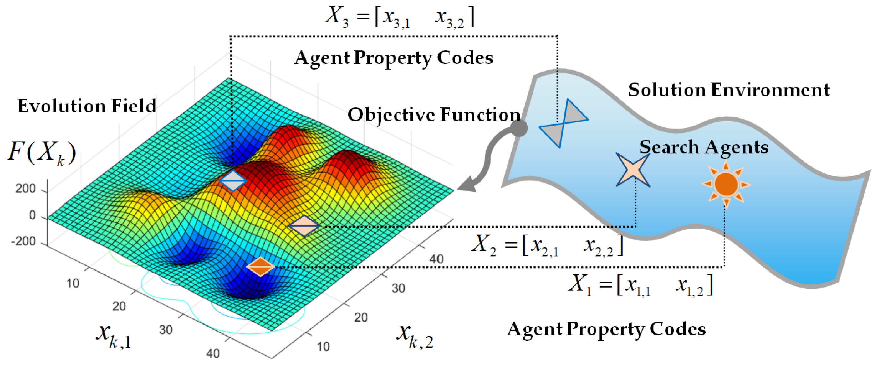
2. Evolutionary Field Search
2.1. Evolutionary Field Theorem of Search Agents
- —the metric expresses dissimilarity of agent properties in the defined metric space. The equality state implies that the agent i and the agent j are the same agent in the solution environment. Values of can express a measure for differentiation of agent properties, and it can be used to evaluate the amount of the evolution of the agent property code;
- —agent properties do not apply any priority;
- —agent properties obey the triangle inequality and it allows to define geometrical evolution strategies. The shortest evolutionary path does not involve any deflection in the code space.
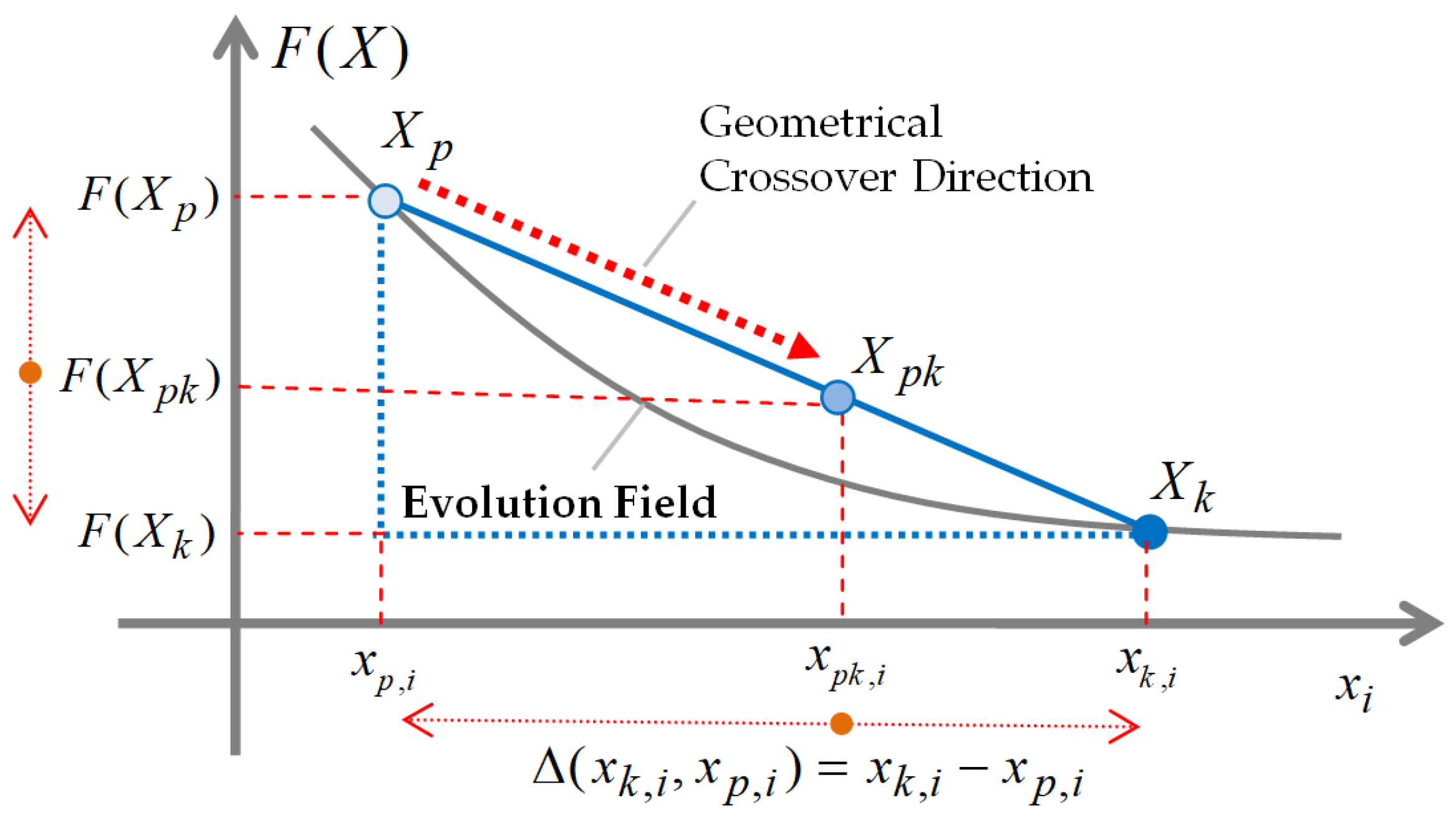
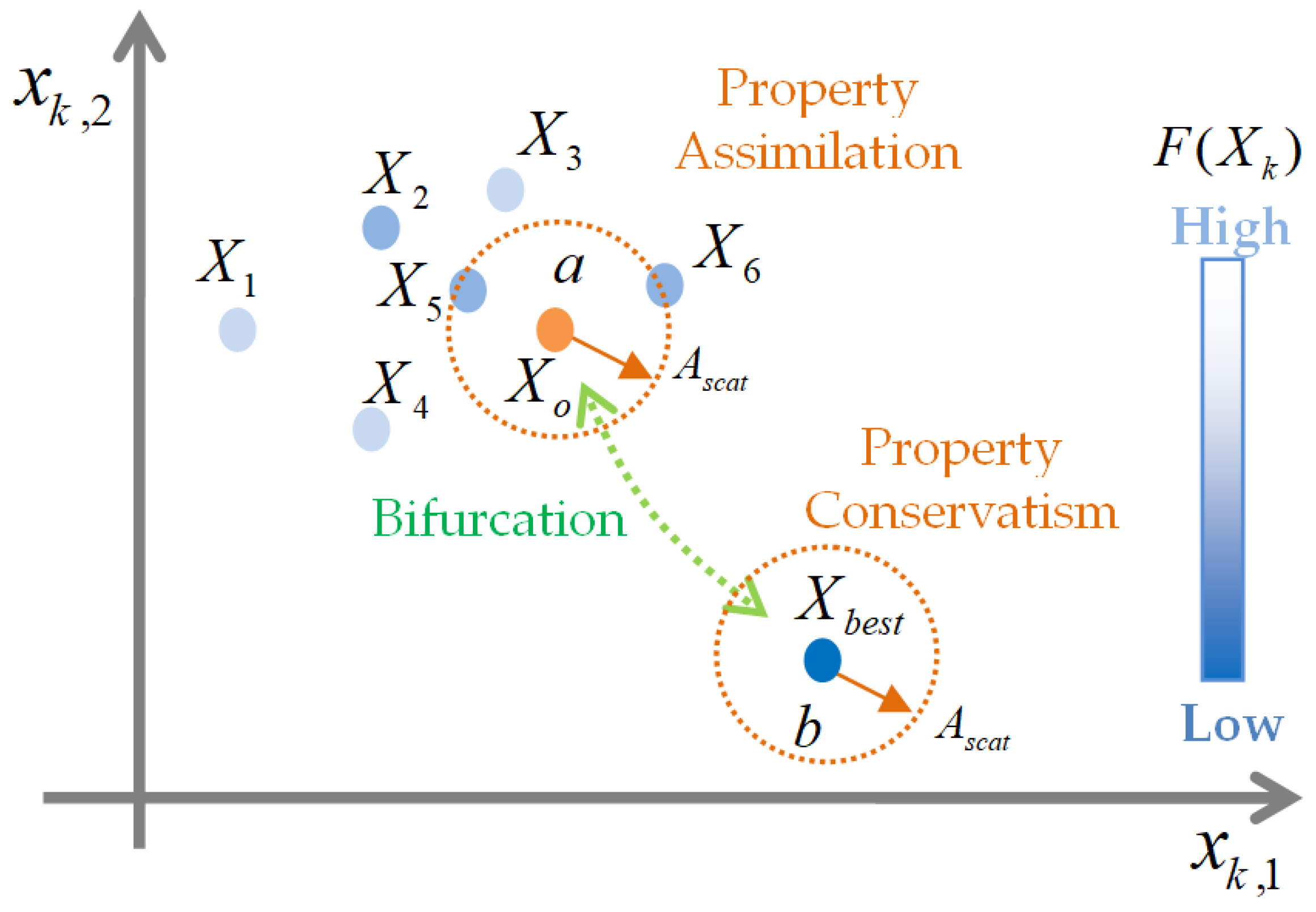
2.2. An Evolutionary Field Optimization with Geometric Strategies
- Step 1
- Randomly distribute all agent property codes within the evolution field;
- Step 2
- Calculate the field values for each property codes ;
- Step 3
- Select the seasonal best agent property code as ;
- Step 4
- Perform the field-adapted differential crossover and field-aware mutation combination for agent property codes according to Equation (15) except the seasonal best agent property code and obtain new generation candidates of the seasonal property codes, ;
- Step 5
- Perform only bifurcated metamutation for the seasonal best agent property code according to Equation (17) and obtain a new generation candidate of the seasonal property code ;
- Step 6
- Form a seasonally evolved new generation set of the seasonal property codes as , and calculate the field values for each new generation property codes from ;
- Step 7
- Select the agent property codes with lower field values from old and new property code collections and update the set of ;
- Step 8
- If a predefined stopping criteria is not met, select the best agent property code with the lowest field value as the optimal solution of the optimization problem. Otherwise, go back to step 3.
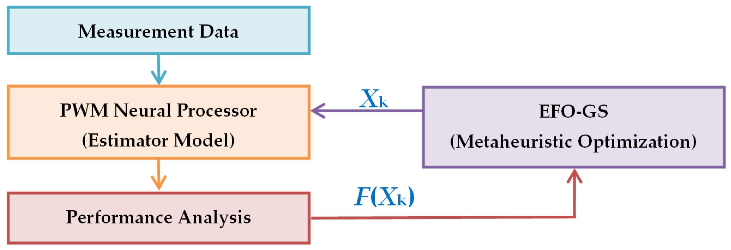
3. Evolutionary Training of Power-Weighted Multiplicative Neural Processor via Evolutionary Field Optimization Algorithm
3.1. Preliminaries for Multiplicative Unit
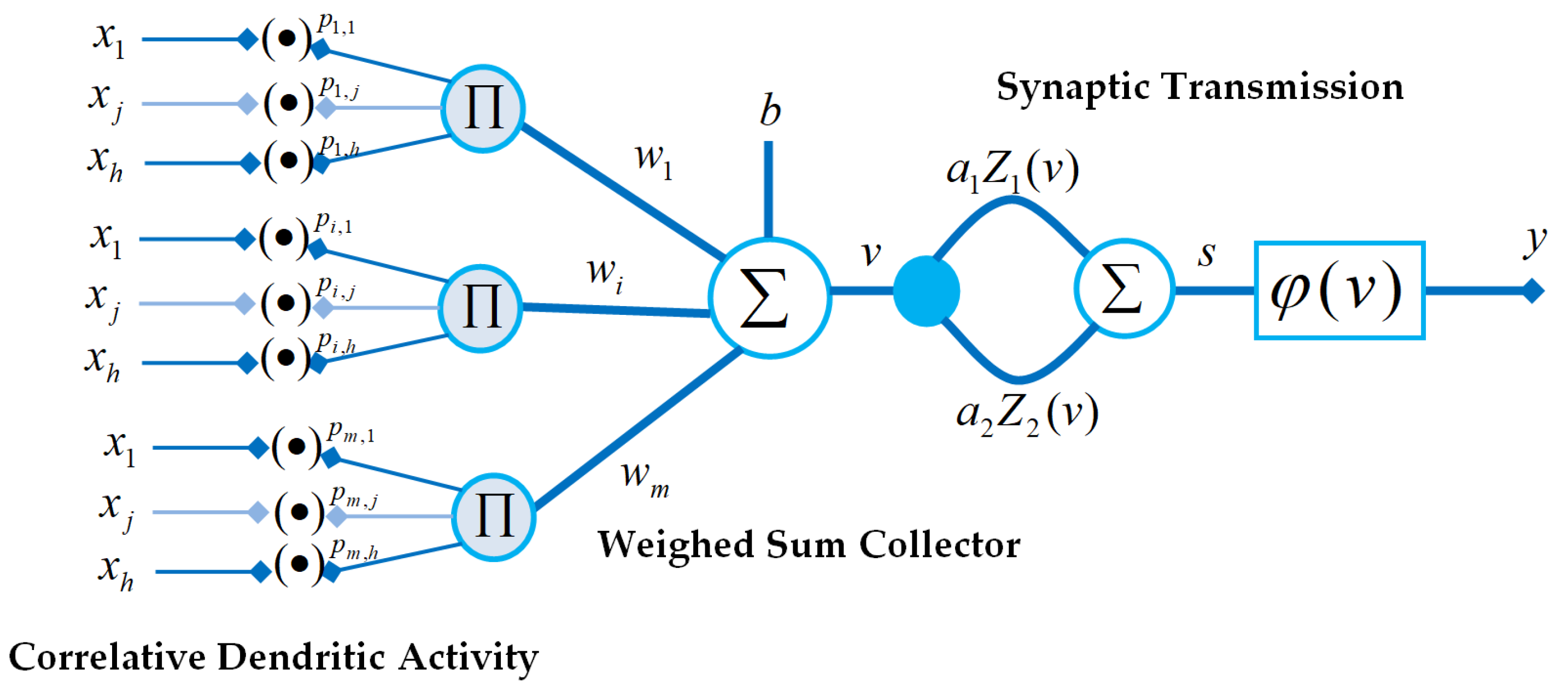
3.2. Power-Weighted Multiplicative Neural Processing
- (i)
- Cartesian () properties: real and imaginary parts of the complex number :
- (ii)
- Polar () properties: magnitude and phase properties of the complex number :
- -
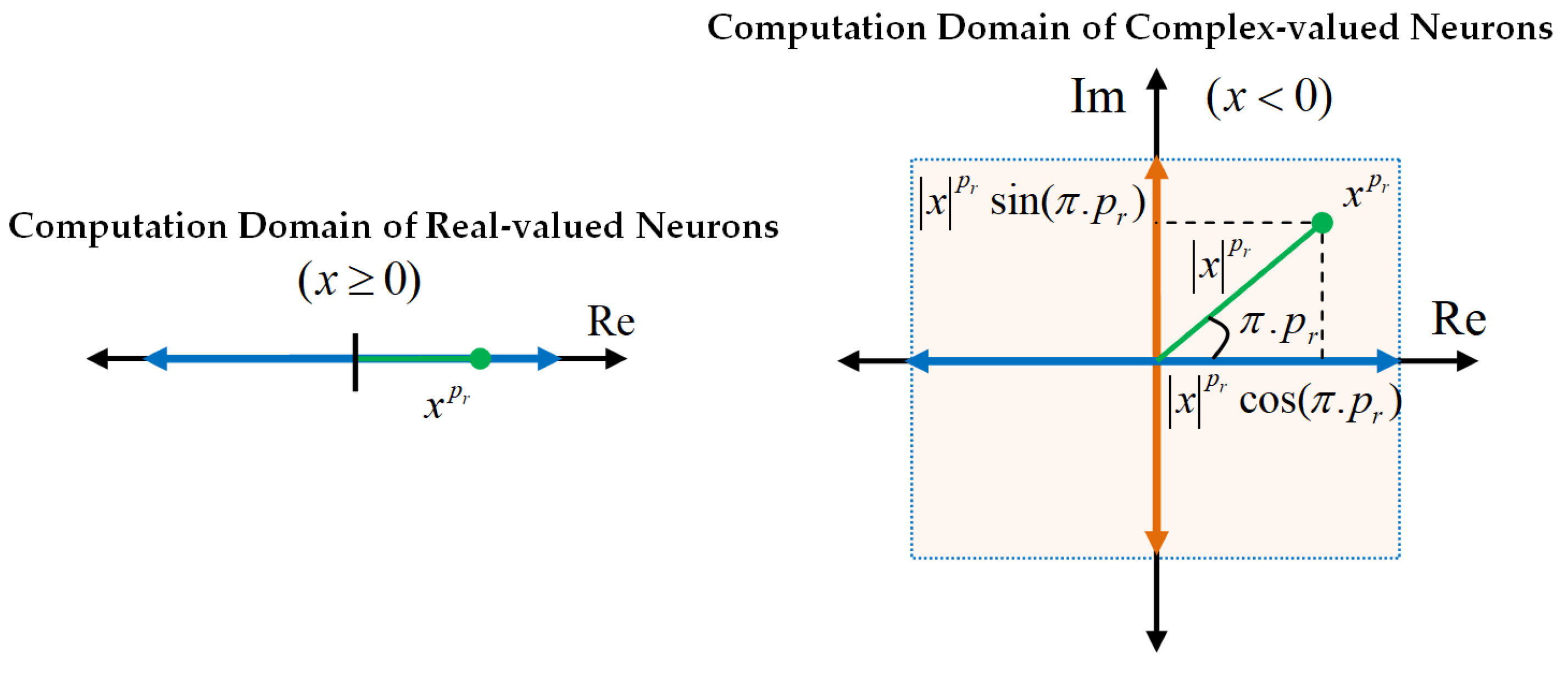
- When or , then it results in and , the PWM neuron operates in the real-valued mode, and its function can be simplified to
- -
- When or , a PWM neuron operates in the complex-valued mode as shown by Equation (28).
4. Experimental Study
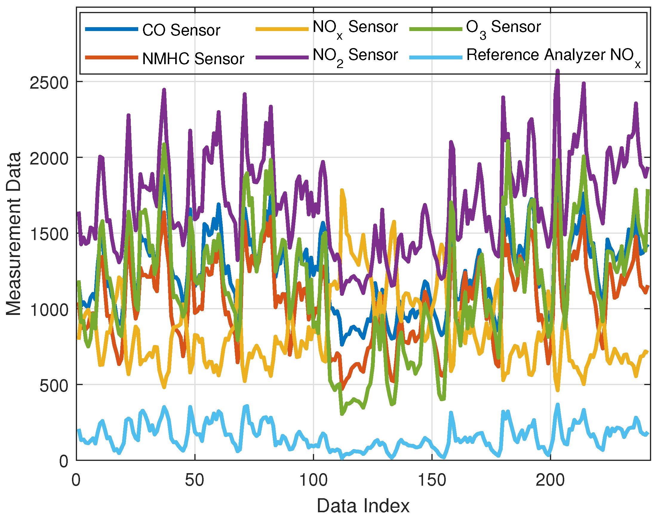
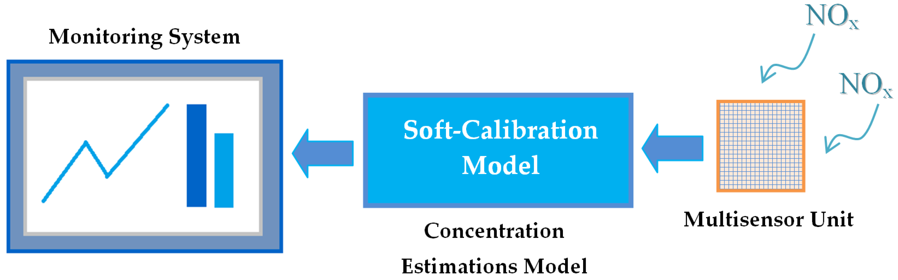
4.1. An Electronic Nose Application for Monitoring NOx Concentration by Solid-State Multisensor Array
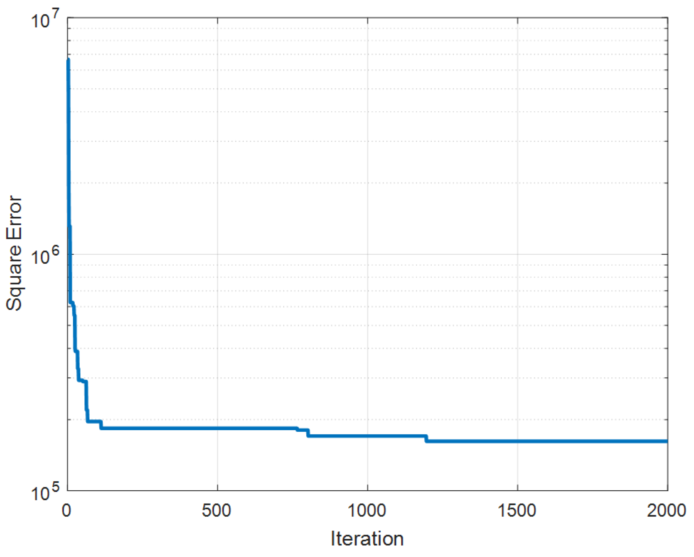
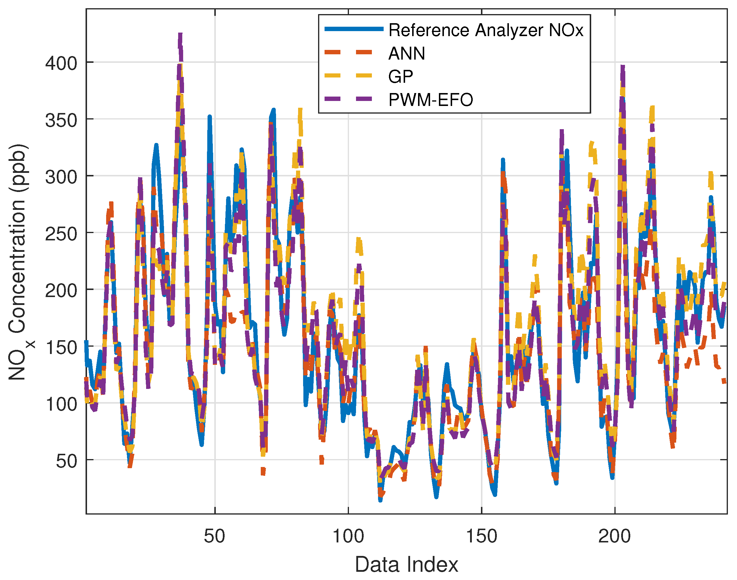
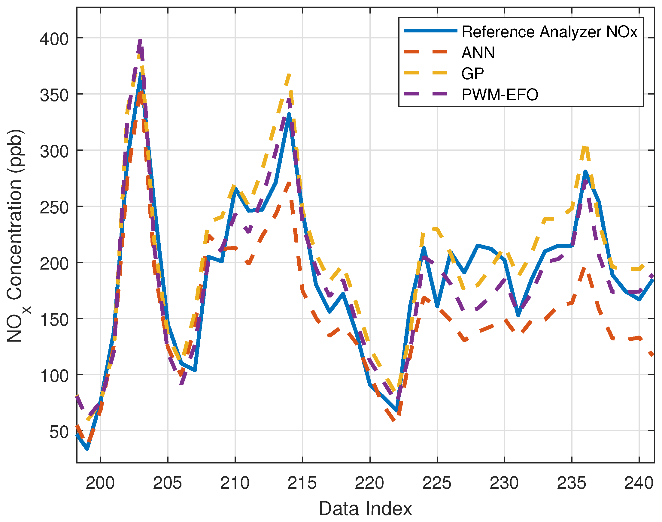
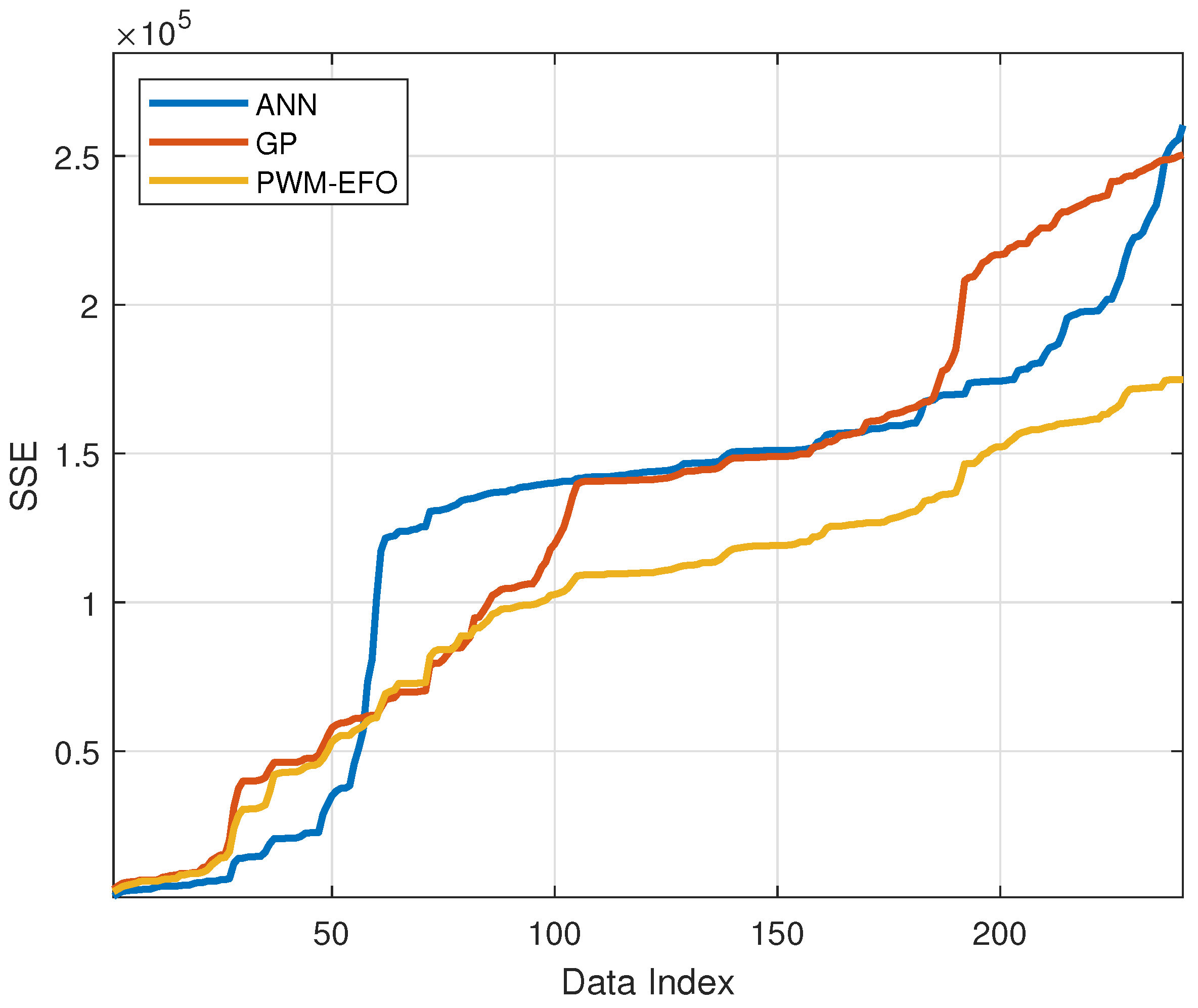
4.2. Experimental Results for Complex-Valued Mode PWM-EFO Neuron
5. Conclusions
Author Contributions
Funding
Institutional Review Board Statement
Informed Consent Statement
Data Availability Statement
Conflicts of Interest
Appendix A
References
- Dasgupta, D.; McGregor, D.R. Designing Application-Specific Neural Networks Using the Structured Genetic Algorithm. In Proceedings of the International Workshop on Combinations of Genetic Algorithms and Neural Networks, COGANN-92s, Baltimore, MD, USA, 6 June 1992; pp. 87–96. [Google Scholar]
- Fong, S.; Deb, S.; Yang, X. How Meta-Heuristic Algorithms Contribute to Deep Learning in the Hype of Big Data Analytics In Progress in Intelligent Computing Techniques: Theory, Practice, and Applications; Springer: Berlin/Heidelberg, Germany, 2008; pp. 3–25. [Google Scholar]
- Galvan, E.; Mooney, P. Neuroevolution in Deep Neural Networks: Current Trends and Future Challenges. IEEE Trans. Artif. Intell. 2021, 2, 476–493. [Google Scholar] [CrossRef]
- Kumar, J.; Singh, A.K. Workload Prediction in Cloud Using Artificial Neural Network and Adaptive Differential Evolution. Future Gener. Comput. Syst. 2018, 81, 41–52. [Google Scholar] [CrossRef]
- Mason, K.; Duggan, J.; Howley, E. A Multi-Objective Neural Network Trained with Differential Evolution for Dynamic Economic Emission Dispatch. Int. J. Electr. Power Energy Syst. 2018, 100, 201–221. [Google Scholar] [CrossRef]
- Stanley, K.O.; Clune, J.; Lehman, J.; Miikkulainen, R. A Multi-Objective Designing Neural Networks through Neuroevolution. Nat. Mach. Intell. 2019, 1, 24–35. [Google Scholar] [CrossRef]
- Ding, S.; Li, H.; Su, C.; Yu, J.; Jin, F. Evolutionary Artificial Neural Networks: A Review. Artif. Intell. Rev. 2013, 39, 251–260. [Google Scholar] [CrossRef]
- Arifovic, J.; Gençay, R. Using Genetic Algorithms to Select Architecture of a Feedforward Artificial Neural Network. Phys. A Stat. Mech. Its Appl. 2001, 289, 574–594. [Google Scholar] [CrossRef]
- Suganuma, M.; Shirakawa, S.; Nagao, T.A. Genetic Programming Approach to Designing Convolutional Neural Network Architectures. In Proceedings of the Genetic and Evolutionary Computation Conference, Berlin, Germany, 15–19 July 2017; pp. 497–504. [Google Scholar]
- Wang, H.; Jin, Y.; Sun, C.; Doherty, J. Offline Data-Driven Evolutionary Optimization Using Selective Surrogate Ensembles. IEEE Trans. Evol. Comput. 2019, 23, 203–216. [Google Scholar] [CrossRef]
- Jin, Y.; Wang, H.; Chugh, T.; Guo, D.; Miettinen, K. Data-Driven Evolutionary Optimization: An Overview and Case Studies. IEEE Trans. Evol. Comput. 2019, 23, 442–458. [Google Scholar] [CrossRef]
- Sexton, R.S.; Gupta, J.N.D. Comparative Evaluation of Genetic Algorithm and Backpropagation for Training Neural Networks. Inf. Sci. 2000, 129, 45–59. [Google Scholar] [CrossRef]
- Che, Z.G.; Chiang, T.A.; Che, Z.H. Feed-Forward Neural Networks Training: A Comparison between Genetic Algorithm and Back-Propagation Learning Algorithm. Int. J. Innov. Comput. 2011, 7, 5839–5850. [Google Scholar]
- Gudise, V.G.; Venayagamoorthy, G.K. Comparison of Particle Swarm Optimization and Backpropagation as Training Algorithms for Neural Networks. In Proceedings of the 2003 IEEE Swarm Intelligence Symposium (SIS’03), Indianapolis, IN, USA, 24–26 April 2003; Cat. No. 03EX706. pp. 110–117. [Google Scholar]
- Ince, T.; Kiranyaz, S.; Pulkkinen, J.; Gabbouj, M.F. Evaluation of Global and Local Training Techniques over Feed-Forward Neural Network Architecture Spaces for Computer-Aided Medical Diagnosis. Expert Syst. Appl. 2010, 37, 8450–8461. [Google Scholar] [CrossRef]
- Mosavi, M.R.; Khishe, M.; Ghamgosar, A. Classification Of Sonar Data Set Using Neural Network Trained By Gray Wolf Optimization. Neural Netw. World 2016, 26, 393–415. [Google Scholar] [CrossRef] [Green Version]
- Ghasemiyeh, R.; Moghdani, R.; Sana, S.S. A Hybrid Artificial Neural Network with Metaheuristic Algorithms for Predicting Stock Price. Cybern. Syst. 2017, 48, 365–392. [Google Scholar] [CrossRef]
- Abdolrasol, M.G.; Hussain, S.M.; Ustun, T.S.; Sarker, M.R.; Hannan, M.A.; Mohamed, R.; Ali, J.A.; Mekhilef, S.; Milad, A. Artificial Neural Networks Based Optimization Techniques: A Review. Electronics 2021, 10, 2689. [Google Scholar] [CrossRef]
- Li, Y.; Wang, S.; Yang, B. An Improved Differential Evolution Algorithm with Dual Mutation Strategies Collaboration. Expert Syst. Appl. 2020, 153, 113451. [Google Scholar] [CrossRef]
- Civicioglu, P.; Besdok, E. ABernstain-Search Differential Evolution Algorithm for Numerical Function Optimization. Expert Syst. Appl. 2019, 138, 112831. [Google Scholar] [CrossRef]
- Sallam, K.M.; Elsayed, S.M.; Chakrabortty, R.K.; Ryan, M.J. Improved Multi-Operator Differential Evolution Algorithm for Solving Unconstrained Problems. In Proceedings of the 2020 IEEE Congress on Evolutionary Computation (CEC), Glasgow, UK, 19–24 July 2020; pp. 1–8. [Google Scholar]
- Yildizdan, G.; Baykan, Ö.K. A Novel Modified Bat Algorithm Hybridizing by Differential Evolution Algorithm. Expert Syst. Appl. 2020, 141, 112949. [Google Scholar] [CrossRef]
- Arce, F.; Zamora, E.; Sossa, H.; Barrón, R. Differential Evolution Training Algorithm for Dendrite Morphological Neural Networks. Appl. Soft Comput. 2018, 68, 303–313. [Google Scholar] [CrossRef]
- Piotrowski, A.P. Differential Evolution Algorithms Applied to Neural Network Training Suffer from Stagnation. Appl. Soft Comput. 2014, 21, 382–406. [Google Scholar] [CrossRef]
- Peng, L.; Liu, S.; Liu, R.; Wang, L. Effective Long Short-Term Memory with Differential Evolution Algorithm for Electricity Price Prediction. Energy 2018, 162, 1301–1314. [Google Scholar] [CrossRef]
- Singh, D.; Kumar, V.; Vaishali; Kaur, M. Classification of COVID-19 Patients from Chest CT Images Using Multi-Objective Differential Evolution–based Convolutional Neural Networks. Eur. J. Clin. Microbiol. Infect. Dis. 2020, 39, 1379–1389. [Google Scholar] [CrossRef] [PubMed]
- Ilonen, J.; Kamarainen, J.K.; Lampinen, J. Differential evolution training algorithm for feed-forward neural networks. Neural Process. Lett. 2003, 17, 93–105. [Google Scholar] [CrossRef]
- Deng, W.; Shang, S.; Cai, X.; Zhao, H.; Song, Y.; Xu, J. An improved differential evolution algorithm and its application in optimization problem. Appl. Soft Comput. 2021, 25, 5277–5298. [Google Scholar] [CrossRef]
- Bäck, T. Evolutionary Algorithms in Theory and Practice; Oxford University Press: Oxford, UK, 1996; ISBN 9780195099713. [Google Scholar]
- Jong, K.D. Evolutionary Computation. Wiley Interdiscip. Rev. Comput. Stat. 2009, 1, 52–56. [Google Scholar] [CrossRef]
- Doerr, B.; Neumann, F. Theory of Evolutionary Computation Doerr; Springer International Publishing: Cham, Switzerland, 2020; ISBN 978-3-030-29413-7. [Google Scholar]
- Papadopoulos, V.; Deodatis, G. Response Variability of Stochastic Frame Structures Using Evolutionary Field Theory. Comput. Methods Appl. Mech. Eng. 2006, 195, 1050–1074. [Google Scholar] [CrossRef]
- Priestley, M.B. Non-Linear and Non-Stationary Time Series Analysis; Acad. Press: London, UK, 1989; ISBN 012564910X. [Google Scholar]
- Priestley, M.B. Evolutionary Spectra and Non-Stationary Processes. J. R. Stat. Soc. Ser. B 1965, 27, 204–229. [Google Scholar] [CrossRef]
- Sutton, R.S.; Barto, A.G. Reinforcement Learning: An Introduction; MIT Press: Cambridge, MA, USA, 2018. [Google Scholar]
- McCulloch, W.S.; Pitts, W. A Logical Calculus of the Ideas Immanent in Nervous Activity. Bull. Math. Biophys. 1943, 5, 115–133. [Google Scholar] [CrossRef]
- Widrow, B.; Lehr, M.A. 30 Years of Adaptive Neural Networks: Perceptron, Madaline, and Backpropagation. Proc. IEEE 1990, 78, 1415–1442. [Google Scholar] [CrossRef]
- Aminian, J.; Shahhosseini, S. Evaluation of ANN Modeling for Prediction of Crude Oil Fouling Behavior. Appl. Therm. Eng. 2008, 28, 668–674. [Google Scholar] [CrossRef]
- Hasanien, H.M. FPGA Implementation of Adaptive ANN Controller for Speed Regulation of Permanent Magnet Stepper Motor Drives. Energy Convers. Manag. 2011, 52, 1252–1257. [Google Scholar] [CrossRef]
- Vijaya, G.; Kumar, V.; Verma, H.K. ANN-Based QRS-Complex Analysis of ECG. J. Med. Eng. Technol. 1998, 22, 160–167. [Google Scholar] [CrossRef] [PubMed]
- Egmont-Petersen, M.; de Ridder, D.; Handels, H. Image Processing with Neural Networks—A Review. Pattern Recognit. 2002, 35, 2279–2301. [Google Scholar] [CrossRef]
- Wilamowski, B.M.; Yu, H. Improved Computation for Levenberg–Marquardt Training. IEEE Trans. Neural Netw. 2010, 21, 930–937. [Google Scholar] [CrossRef] [PubMed]
- Nawi, N.M.; Khan, A.; Rehman, M.Z. A New Levenberg Marquardt Based Back Propagation Algorithm Trained with Cuckoo Search. Procedia Technol. 2013, 11, 18–23. [Google Scholar] [CrossRef] [Green Version]
- Hagan, M.T.; Menhaj, M.B. Training Feedforward Networks with the Marquardt Algorithm. IEEE Trans. Neural Netw. 1994, 5, 989–993. [Google Scholar] [CrossRef]
- Bingham, G.; Miikkulainen, R. Discovering Parametric Activation Functions. Neural Netw. 2022, 148, 48–65. [Google Scholar] [CrossRef]
- Giles, C.L.; Maxwell, T. Learning, Invariance, and Generalization in High-Order Neural Networks. Appl. Opt. 1987, 26, 4972. [Google Scholar] [CrossRef]
- Durbin, R.; Rumelhart, D.E. Product Units: A Computationally Powerful and Biologically Plausible Extension to Backpropagation Networks. Neural Comput. 1989, 1, 133–142. [Google Scholar] [CrossRef]
- Leerink, L.; Giles, C.; Horne, B.; Jabri, M.A. Learning with Product Units. Adv. Neural Inf. Process. Syst. 1994, 7, 537–544. [Google Scholar]
- Schmitt, M. On the Complexity of Computing and Learning with Multiplicative Neural Networks. Neural Comput. 2002, 14, 241–301. [Google Scholar] [CrossRef]
- Salinas, E.; Abbott, L.F. A Model of Multiplicative Neural Responses in Parietal Cortex. Proc. Natl. Acad. Sci. USA 1996, 93, 11956–11961. [Google Scholar] [CrossRef] [PubMed] [Green Version]
- Simon, J. Multiplicative Neural Networks. Available online: https://james-simon.github.io/deeplearning/2020/08/31/multiplicative-neural-nets (accessed on 18 March 2022).
- Oh, S.-K.; Pedrycz, W.; Park, B.-J. Polynomial Neural Networks Architecture: Analysis and Design. Comput. Electr. Eng. 2003, 29, 703–725. [Google Scholar] [CrossRef]
- Chrysos, G.G.; Moschoglou, S.; Bouritsas, G.; Panagakis, Y.; Deng, J.; Zafeiriou, S. Deep Polynomial Neural Networks. In Proceedings of the 2020 IEEE/CVF Conference on Computer Vision and Pattern Recognition (CVPR), Seattle, WA, USA, 13–19 June 2020; pp. 7323–7333. [Google Scholar]
- Morala, P.; Cifuentes, J.A.; Lillo, R.E.; Ucar, I. Towards a Mathematical Framework to Inform Neural Network Modelling via Polynomial Regression. Neural Netw. 2021, 142, 57–72. [Google Scholar] [CrossRef] [PubMed]
- Neri, F.; Cotta, C. Memetic algorithms and memetic computing optimization: A literature review. Swarm Evol. Comput. 2012, 2, 1–14. [Google Scholar] [CrossRef]
- Doğan, B. A modified vortex search algorithm for numerical function optimization. arXiv 2016, arXiv:1606.02710. [Google Scholar]
- Bergou, E.H.; Gorbunov, E.; Richtárik, P. Stochastic three points method for unconstrained smooth minimization. SIAM J. Optim. 2019, 30, 2726–2749. [Google Scholar] [CrossRef]
- Bagattini, F.; Schoen, F.; Tigli, L. Clustering methods for large scale geometrical global optimization. Optim. Methods Softw. 2019, 34, 1099–1122. [Google Scholar] [CrossRef]
- Dunning, T. Recorded Step Directional Mutation for Faster Convergence. In Proceedings of the International Conference on Evolutionary Programming, San Diego, CA, USA, 25–27 March 1998; pp. 569–578. [Google Scholar]
- Bedau, M.A.; Seymour, R. Adaptation of Mutation Rates in a Simple Model of Evolution. In Complex Systems: Mechanism of Adaptation; IOS Press: Amsterdam, The Netherlands, 1995; pp. 37–44. [Google Scholar]
- Tokumoto, S.; Yoshida, H.; Sakamoto, K.; Honiden, S. MuVM: Higher Order Mutation Analysis Virtual Machine for C. In Proceedings of the 2016 IEEE International Conference on Software Testing, Verification and Validation (ICST), Chicago, IL, USA, 11–15 April 2016; pp. 320–329. [Google Scholar]
- Whitley, D.; Starkweather, T.; Bogart, C. Genetic Algorithms and Neural Networks: Optimizing Connections and Connectivity. Parallel Comput. 1990, 14, 347–361. [Google Scholar] [CrossRef]
- Zbigniew, M. Genetic Algorithms + Data Structures = Evolution Programs; Springer: Berlin/Heidelberg, Germany, 1992. [Google Scholar]
- Ren, Z.; San, Y. Improvement of Real-Valued Genetic Algorithm and Performance Study. Acta Electron. Sin. 2007, 35, 269–274. [Google Scholar]
- Meng, X.; Zhang, H.; Tan, W. A Hybrid Method of GA and BP for Short-Term Economic Dispatch of Hydrothermal Power Systems. Math. Comput. Simul. 2000, 51, 341–348. [Google Scholar] [CrossRef]
- Whitley, D. An Overview of Evolutionary Algorithms: Practical Issues and Common Pitfalls. Inf. Softw. Technol. 2001, 43, 817–831. [Google Scholar] [CrossRef]
- Yao, X.; Liu, Y. A New Evolutionary System for Evolving Artificial Neural Networks. IEEE Trans. Neural Netw. 1997, 8, 694–713. [Google Scholar] [CrossRef] [PubMed] [Green Version]
- Yan, J.; Guo, X.; Duan, S.; Jia, P.; Wang, L.; Peng, C.; Zhang, S. Electronic Nose Feature Extraction Methods. Sensors 2015, 15, 27804–27831. [Google Scholar] [CrossRef] [PubMed]
- Benedetti, S.; Mannino, S.; Sabatini, A.G.; Marcazzan, G.L. Electronic nose and neural network use for the classification of honey. Apidologie 2004, 35, 397–402. [Google Scholar] [CrossRef] [Green Version]
- De Vito, S.; Piga, M.; Martinotto, L.; Di Francia, G. CO, NO2 and NOx Urban Pollution Monitoring with on-Field Calibrated Electronic Nose by Automatic Bayesian Regularization. Sens. Actuators B Chem. 2009, 143, 182–191. [Google Scholar] [CrossRef]
- De Vito, S.; Massera, E.; Piga, M.; Martinotto, L.; Di Francia, G. On Field Calibration of an Electronic Nose for Benzene Estimation in an Urban Pollution Monitoring Scenario. Sens. Actuators B Chem. 2008, 129, 750–757. [Google Scholar] [CrossRef]
- Zhang, L.; Tian, F.; Liu, S.; Guo, J.; Hu, B.; Ye, Q.; Dang, L.; Peng, X.; Kadri, C.; Feng, J. Chaos based neural network optimization for concentration estimation of indoor air contaminants by an electronic nose. Sens. Actuators A Phys. 2013, 189, 161–167. [Google Scholar] [CrossRef]
- Seesaard, T.; Goel, N.; Kumar, M.; Wongchoosuk, C. Advances in gas sensors and electronic nose technologies for agricultural cycle applications. Comput. Electron. Agric. 2022, 193, 106673. [Google Scholar] [CrossRef]
- Seesaard, T.; Thippakorn, C.; Kerdcharoen, T.; Kladsomboon, S. A hybrid electronic nose system for discrimination of pathogenic bacterial volatile compounds. Anal. Methods 2020, 12, 5671–5683. [Google Scholar] [CrossRef]
- Forman, E.; Peniwati, K. Aggregating Individual Judgments and Priorities with the Analytic Hierarchy Process. Eur. J. Oper. Res. 1998, 108, 165–169. [Google Scholar] [CrossRef]
- Chiclana, F.; Herrera, F.; Herrera-Viedma, E. Integrating Multiplicative Preference Relations in a Multipurpose Decision-Making Model Based on Fuzzy Preference Relations. Fuzzy Sets Syst. 2001, 122, 277–291. [Google Scholar] [CrossRef]
- Herrera, F.; Herrera-Viedma, E.; Chiclana, F. Multiperson Decision-Making Based on Multiplicative Preference Relations. Eur. J. Oper. Res. 2001, 129, 372–385. [Google Scholar] [CrossRef]
- Liu, F.; Zhang, W.-G.; Zhang, L.-H. A Group Decision Making Model Based on a Generalized Ordered Weighted Geometric Average Operator with Interval Preference Matrices. Fuzzy Sets Syst. 2014, 246, 1–18. [Google Scholar] [CrossRef]
- Kerlin, A.; Mohar, B.; Flickinger, D.; MacLennan, B.J.; Dean, M.B.; Davis, C.; Spruston, N.; Svoboda, K. Functional Clustering of Dendritic Activity during Decision-Making. eLife 2019, 8, 1–32. [Google Scholar] [CrossRef]
- Bassey, J.; Qian, L.; Li, X. A Survey of Complex-Valued Neural Networks. arXiv 2021, arXiv:2101.12249. [Google Scholar]
- Skowron, A.; Lee, D.S.; De León, R.R.; Lim, L.L.; Owen, B. Greater Fuel Efficiency Is Potentially Preferable to Reducing NOx Emissions for Aviation’s Climate Impacts. Nat. Commun. 2021, 12, 564. [Google Scholar] [CrossRef]
- Gangisetty, G.; Ivchenko, A.V.; Thomas Jayachandran, A.V.; Sverbilov, V.Y.; Matveev, S.S.; Chechet, I.V. Methodology Development for the Control of NOx Emissions in Aerospace Industry. J. Phys. Conf. Ser. 2019, 1276, 12075. [Google Scholar] [CrossRef] [Green Version]
- Tsujita, W.; Yoshino, A.; Ishida, H.; Moriizumi, T. Gas Sensor Network for Air-Pollution Monitoring. Sens. Actuators B Chem. 2005, 110, 304–311. [Google Scholar] [CrossRef]
- Capelli, L.; Sironi, S.; Del Rosso, R. Electronic Noses for Environmental Monitoring Applications. Sensors 2014, 14, 19979–20007. [Google Scholar] [CrossRef]
- Madár, J.; Abonyi, J.; Szeifert, F. Genetic Programming for the Identification of Nonlinear Input–Output Models. Ind. Eng. Chem. Res. 2005, 44, 3178–3186. [Google Scholar] [CrossRef]


| Metaheuristic Methods | Advantages | Disadvantages |
|---|---|---|
| PSO | For the training of shallow neural networks, the PSO can present faster convergence than backpropagation algorithms [14] and perform global searching [15]. | Although performing a global search, it is possible to converge to local minima. Inappropriate selection of hyper-parameters of PSO may produce relatively poor results [18]. |
| GA | The GA can provide better training performance than backpropagation algorithms [13] because GA performs a gradient-free optimization [15] and global search. It can be effective for training of shallow neural networks. | The convergence to minimum solution can take longer when hyper-parameters are not well tuned [18]. |
| DE | It can perform global searching in the training [23] and find optimal ANN training solutions at the expense of more computation time [27]. | The DE algorithm may cause premature convergence and poor performance [18,28]. |
| Intervals | Operation Modes | Interval Reversing to Switch between Operation Modes |
|---|---|---|
| Complex-valued Neuron | When in the real valued mode, use as input data because | |
| Real-valued Neuron | When in the complex valued mode, use as input data because | |
| and | Mixed-mode Neuron | It operates the mixed-mode when input data have positive and negative values |
| Proper Parameter Configuration | Neural Network Model | Model Formulation |
|---|---|---|
| None | PWM neuron model | , , |
| , , , and | McCulloch and Pitts classical neuron model | , , |
| , , and | Polynomial neurons | , , |
| Sensor Types | Data Types | Explanation | Parameters |
|---|---|---|---|
| PT08.S1 | Input | Tin oxide gas sensor (CO sensitive) | |
| PT08.S2 | Input | Titania gas sensor (NMHC sensitive) | |
| PT08.S3 | Input | Tungsten oxide gas sensor (NOx sensitive) | |
| PT08.S4 | Input | Tungsten oxide gas sensor (NO2 sensitive) | |
| PT08.S5 | Input | Indium oxide gas sensor (O3 sensitive) | |
| Temperature | Input | Temperature Measurement °C | |
| Relative Humidity | Input | Relative Humidity Measurement (%) | |
| Absolute Humidity | Input | Absolute Humidity | |
| Reference Analyzer | Ground truth data | True concentration measurements for NOx (ppb) |
| Estimation Models | MSE | MAE | MRE | R2 |
|---|---|---|---|---|
| ANN | 1079.7 | 22.8 | 0.15 | 0.84 |
| GP | 1038.9 | 24.6 | 0.18 | 0.84 |
| PWM-EFO | 725.52 | 20.8 | 0.16 | 0.89 |
| Estimation Models | Mean | Standard Deviation |
|---|---|---|
| ANN | 11.9 | 30.6 |
| GP | −6.9 | 31.5 |
| PWM-EFO | 2.75 | 26.8 |
| Estimation Models | MSE | MAE | MRE | R2 |
|---|---|---|---|---|
| PWM-EFO (Real) | 725.52 | 20.8 | 0.16 | 0.89 |
| PWM-EFO (Complex) | 842.46 | 22.9 | 0.18 | 0.87 |
Publisher’s Note: MDPI stays neutral with regard to jurisdictional claims in published maps and institutional affiliations. |
© 2022 by the authors. Licensee MDPI, Basel, Switzerland. This article is an open access article distributed under the terms and conditions of the Creative Commons Attribution (CC BY) license (https://creativecommons.org/licenses/by/4.0/).
Share and Cite
Alagoz, B.B.; Simsek, O.I.; Ari, D.; Tepljakov, A.; Petlenkov, E.; Alimohammadi, H. An Evolutionary Field Theorem: Evolutionary Field Optimization in Training of Power-Weighted Multiplicative Neurons for Nitrogen Oxides-Sensitive Electronic Nose Applications. Sensors 2022, 22, 3836. https://doi.org/10.3390/s22103836
Alagoz BB, Simsek OI, Ari D, Tepljakov A, Petlenkov E, Alimohammadi H. An Evolutionary Field Theorem: Evolutionary Field Optimization in Training of Power-Weighted Multiplicative Neurons for Nitrogen Oxides-Sensitive Electronic Nose Applications. Sensors. 2022; 22(10):3836. https://doi.org/10.3390/s22103836
Chicago/Turabian StyleAlagoz, Baris Baykant, Ozlem Imik Simsek, Davut Ari, Aleksei Tepljakov, Eduard Petlenkov, and Hossein Alimohammadi. 2022. "An Evolutionary Field Theorem: Evolutionary Field Optimization in Training of Power-Weighted Multiplicative Neurons for Nitrogen Oxides-Sensitive Electronic Nose Applications" Sensors 22, no. 10: 3836. https://doi.org/10.3390/s22103836
APA StyleAlagoz, B. B., Simsek, O. I., Ari, D., Tepljakov, A., Petlenkov, E., & Alimohammadi, H. (2022). An Evolutionary Field Theorem: Evolutionary Field Optimization in Training of Power-Weighted Multiplicative Neurons for Nitrogen Oxides-Sensitive Electronic Nose Applications. Sensors, 22(10), 3836. https://doi.org/10.3390/s22103836