Article

Model of Magnetically Shielded Ferrite-Cored Eddy Current Sensor

1
Faculty of Electrical Engineering and Computing, University of Zagreb, 10000 Zagreb, Croatia
2
INETEC Institute for Nuclear Technology, 10250 Zagreb, Croatia
*
Author to whom correspondence should be addressed.
Sensors 2022, 22(1), 326; https://doi.org/10.3390/s22010326
Submission received: 26 November 2021 / Revised: 25 December 2021 / Accepted: 28 December 2021 / Published: 2 January 2022

Abstract

:
Computationally fast electromagnetic models of eddy current sensors are required in model-based measurements, machine interpretation approaches or in the sensor design phase. If a sensor geometry allows it, the analytical approach to the modeling has significant advantages in comparison to numerical methods, most notably less demanding implementation and faster computation. In this paper, we studied an eddy current sensor consisting of a transmitter coil with a finitely long I ferrite core, which was screened with a finitely thick magnetic shield. The sensor was placed above a conductive and magnetic half-layer. We used vector magnetic potential formulation of the problem with a truncated region eigenfunction expansion, and obtained expressions for the transmitter coil impedance and magnetic potential in all subdomains. The modeling results are in excellent agreement with the results using the finite element method. The model was also compared with the impedance measurement in the frequency range from 5 kHz to 100 kHz and the agreement is within 3 % for the resistance change due to the presence of the half-layer and 1 % for the inductance change. The presented model can be used for measurement of properties of metallic objects, sensor lift-off or nonconductive coating thickness.

1. Introduction

Eddy current sensors (probes) respond to changes in the material properties (electrical conductivity, magnetic permeability), geometry or position of the nearby electrically conductive, usually metallic, objects [1,2]. Their applications include nondestructive testing for defects and material changes in objects, such as heat exchangers in nuclear plants, oil well casings, pipelines or aircraft hulls [3,4,5]; measurement of the distance to such objects or their dimensions [6,7]; and material characterization [8,9,10]. Eddy current sensors offer detection of very small surface defects, measurement of dimensions or distances in the micrometer range, insensitivity to nonconductive dirt, such as oil, water or dust, and robustness to the environmental factors such as pressure, temperature or stress. However, absolute measurement using eddy current sensors can be hard to achieve leading to the need for calibration, and human or machine analysis and interpretation of the sensor signals [11,12,13].
Traditionally, an eddy current sensor consists of a transmitter coil that generates a magnetic field and induces the eddy currents in the conductive material [1]. Receiver coils pick up the resultant magnetic field due to the defect and changes in the dimensions and material properties. Receiver coils can be replaced by Hall, magnetoresistive or even super-conducting quantum interference devices (SQUID) sensors [14]. However, the overall characteristics of the eddy current sensors are primarily determined by the excitation, geometry and construction of the transmitter coil.
Fast electromagnetic models of transmitter coils are required in model-based measurements, machine interpretation approach or in parametric and sensitivity analyses in the sensor design phase. When it comes to more complicated sensor geometries, analytical electromagnetic models are not as versatile as numerical ones, e.g., finite-element or boundary-element models. However, if a real sensor and object under test can be approximated by a geometry that is simple enough to be dealt with analytically, then one can expect less demanding numerical implementation and higher computational speed in comparison to fully numerical approaches. More complicated geometries can be treated using hybrid approaches in which the analytical models are used for calculation of the incidence fields and numerical methods for calculation of the fields scattered from the small changes in the tested object [15].
Typically with eddy current sensors, the transmitter coil has a ferrite core to increase the inductance, sensitivity and signal-to-noise ratio or to achieve the desired magnetic field distribution. Since the seminal work by Dodd and Deeds [16], who studied air-cored transmitter coils in planar and cylindrical geometries (layers, rods, tubes), a number of more complicated geometries have been analyzed using the truncated region eigenfunction expansion approach (TREE) [17]. This includes ferrite-cored transmitter coils, which previously required numerical or empirical approaches. In a paper that laid out the modeling path followed by other authors, Theodoulidis analyzed the coil with the cylindrical finite-length ferrite core that was positioned above a half space made of two nonmagnetic and conductive layers [18]. This analysis was extended to a half space made of multiple magnetic and conductive layers by Lu et al. in [19]. Bayani et al., in [20], developed the model of a cup-cored coil above a nonmagnetic conductive double layered half space. In all three studies, the models were verified experimentally and the relative error between the theoretical results and measurements were on average between 0.5 % and 2.5 % . Sakkaki and Bayani, in [21], modeled an E-cored coil above a conductive double layer, and they numerically verified the model by comparing it to a finite element model using Comsol. Tytko and Dziczkowski, in [22,23,24], modeled the I-cored and E-cored coils in the presence of the layered medium with a hole, and they verified their work using a Comsol-based finite element model. Zhu et al., in [25], analyzed an I-cored coil screened with a thin sheet of material with infinite permeability.
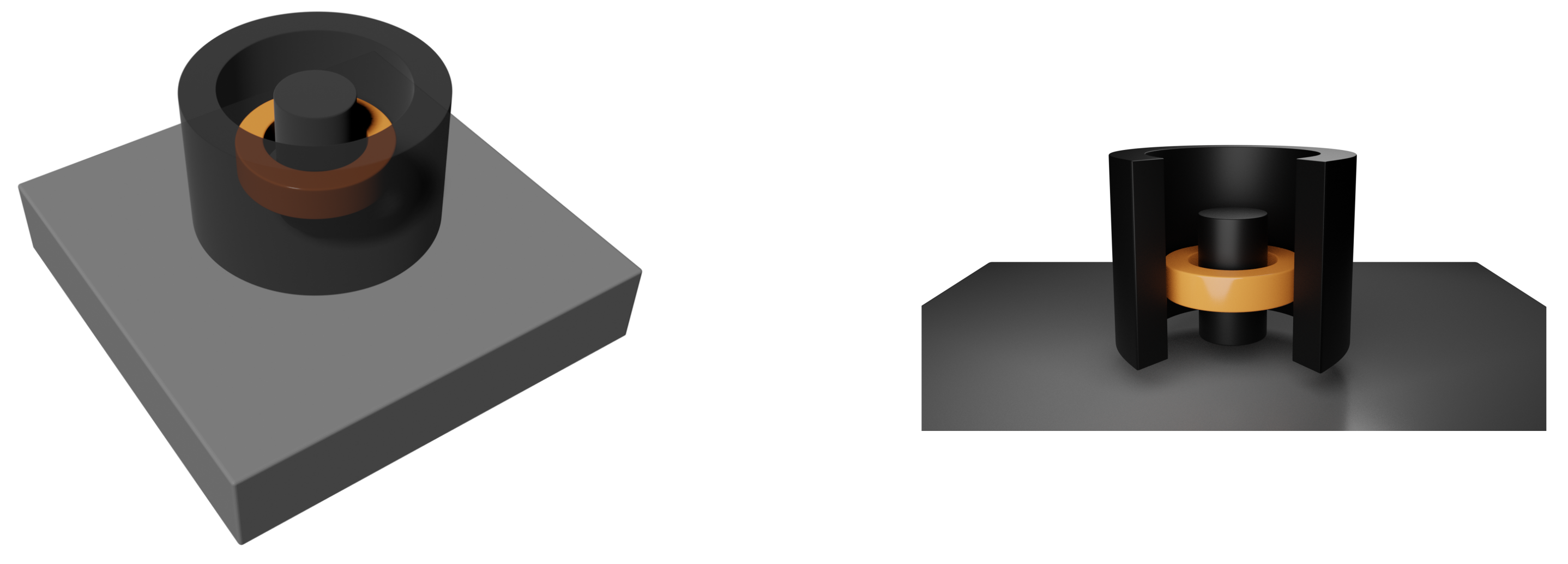
In this paper, we studied a coil with a finitely long I core and screened with a finitely thick magnetic shield placed above a conductive and magnetic half-layer using the TREE approach. Figure 1 and Figure 2 depict the geometry in more detail. We made no assumptions regarding the shield thickness and the permeability of the shield and the core. The open upper side of the shield allows for the coil wires and connector towards a measurement instrument. This sensor geometry is typical and practically important, but to the best of our knowledge it was not modeled analytically before. The contributions of this paper are the analytical model of the sensor impedance above a plate made of conductive and magnetic material in Section 2 and accompanied Appendix A, analysis of numerical implementation issues in Section 3, comparison with a finite element model in Section 4, experimental verification in Section 5 and sensitivity analysis with respect to the sensor dimension in Section 6. The immediate application of these contributions could allow model-based measurement of material properties and lift-off (e.g., nonconductive coating thickness) with no or less calibration points (measurement above reference standards with known material and lift-off) compared to the existing measurement procedures [26]. The model can also be used in the sensor design phase where it is often necessary to adjust the sensor properties to the specific application or account for sensor production tolerances. Furthermore, we believe that the modeling approach and discussion on the implementation issues can be useful in modeling other similar induction sensors with ferrites.
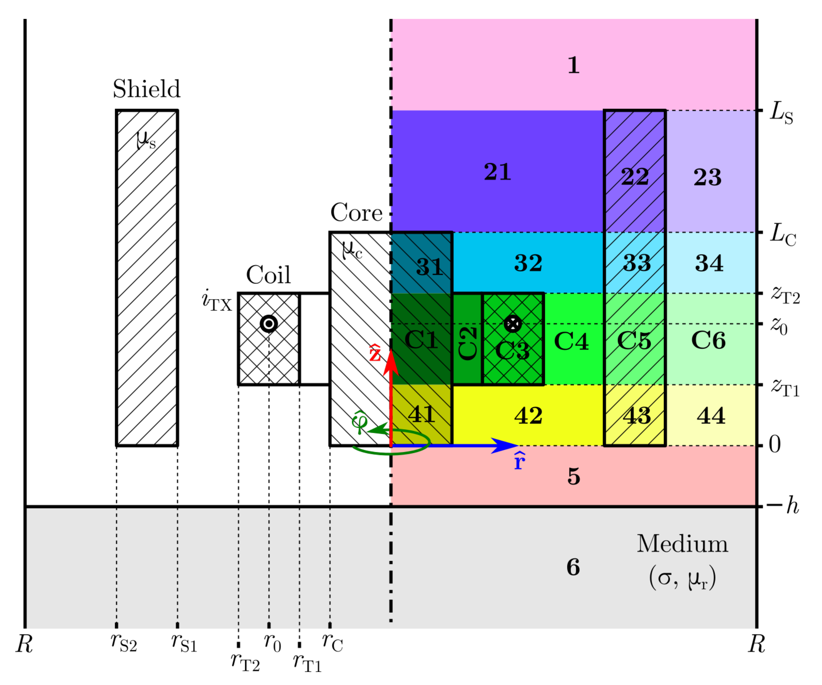
2. Analysis

The geometry of the problem is shown in Figure 1 and Figure 2. The coil with a rectangular cross section is wound around the ferrite core with relative magnetic permeability μ C . The coil and its core are screened with the ferrite shield with relative magnetic permeability μ S . The core and the shield are vertically aligned at the plane z = 0 . The core and the shield are assumed to be nonconductive. The sensor is located over the magnetic and conductive half space (plate) with electrical conductivity σ and relative magnetic permeability μ r .
Before we derive the vector magnetic potential of the coil, we will first analyze a filamentary sinusoidal current I exp j ω t δ r r 0 δ z z 0 φ ^ , where δ is the Dirac delta function and φ ^ is the azimuthal unit vector for the cylindrical coordinate system. The problem is axially symmetric, so there is only φ component of the vector magnetic potential, i.e., A r , z = A r , z φ ^ .
The problem domain is truncated at far enough boundary r = R , where we will impose the Dirichlet boundary condition A r = R , z = 0 . The consequence of the truncation is that the final expressions for the potential are in series rather than integral form. The problem domain is divided into horizontal regions indicated generally by index n in the expressions, or specifically by a number or the letter C. If there are multiple materials or the coil in a region, the region is divided into subregions that are indicated generally by index m or specifically by a number following the region designation. For example, A 1 is the potential in region 1 (no subregions) and A 23 in region 2, subregion 3.
Following the separation of variables, the general form of the magnetic potential is
A n r , z = i = 1 R n α n , i r Z n β n , i z = = i = 1 U n , i J 1 α n , i r + V n , i Y 1 α n , i r C n , i exp β n , i z + D n , i exp β n , i z , for n 1 , 5 , 6 ,
A n m r , z = i = 1 R n m α n , i r Z n α n , i z = = i = 1 U n m , i J 1 α n , i r + V n m , i Y 1 α n , i r C n , i exp α n , i z + D n , i exp α n , i z , for n 2 , 3 , 4 , C ,
where J 1 and Y 1 are first-order Bessel functions of the first and second kind, respectively, α n , i are eigenvalues arising from the Dirichlet boundary condition at r = R for each region, Section 2.2, and
β n , i = α n , i 2 + j ω μ 0 μ n σ n .
If a region is homogeneous with relative permeability μ n and conductivity σ n , i.e., it has no multiple subregions, the form of the potential is given by (1). For regions with multiple subregions, the general form of the potential in subregion m of region n with relative permeability μ n m is given by (2). It is important for further steps to note that there are no conductive materials in the regions with multiple subregions (only air or ferrites) and that, consequently, both r-related and z-related parts have the same eigenvalues α n , i . This means that z-related parts of the subregions in a given region are the same in case of (2).
The homogeneous regions n 1 , 5 , 6 have their corresponding coefficients V i = 0 because of the divergence of Y 1 at r = 0 , so, consequently, one can freely set U i = 1 . Coefficients U n m , i and V n m , i in (2) for regions n 2 , 3 , 4 , C are determined from the interface conditions along the radial boundaries between the subregions, as described in Section 2.1. The interface conditions in this case are continuity of B r and H z , i.e., component of B in r ^ direction, and component of H in z ^ direction.
The unknown coefficients C n , i and D n , i in (1) and (2) are determined from the boundary and interface conditions along the horizontal boundaries between the regions, Section 2.4. The potential must remain finite as z ± , so D 1 , i = 0 and C 6 , i = 0 . The interface conditions for the horizontal boundaries are continuity of B z and H r .

2.1. Continuity of B r and H z at Radial Boundaries between Subregions

This condition has to be satisfied for regions 2, 3 and 4. We will analyze a general case of a region n with subregions m = 1 , , M and radial interfaces between these subregions at r n 1 , , r n ( M 1 ) . In that case, the radial parts under the sum in (2) for each subregion are
R n 1 α n , i r = J 1 α n , i r , 0 r r n 1 ,
R n 2 α n , i r = U n 2 , i J 1 α n , i r + V n 2 , i Y 1 α n , i r , r n 1 < r r n 2 ,
R n m α n , i r = U n m , i J 1 α n , i r + V n m , i Y 1 α n , i r , r n ( m 1 ) < r r n m ,
R n M α n , i r = U n M , i J 1 α n , i r + V n M , i Y 1 α n , i r , r n ( M 1 ) < r R , r n M = R .
For the two neighboring subregions m and m + 1 , the radial interface of continuity of B r and H z at r = r n m is equivalent to
A n m r n m , z = A n ( m + 1 ) r n m , z ,
1 μ n m A n m r + A n m r | r = r n m = 1 μ n ( m + 1 ) A n ( m + 1 ) r + A n ( m + 1 ) r | r = r n m .
Since all subregions in region n have the same z-related part, the radial interface conditions can be satisfied by adjusting the coefficients of the r-related part only. The notation will be simpler if we define matrix R as
R α n , i r n m , μ n m = J 1 α n , i r n m Y 1 α n , i r n m J 0 α n , i r n m / μ n m Y 0 α n , i r n m / μ n m .
It can be shown using (2)–(10) that the coefficients in the r-related part of subregion m + 1 are connected to the coefficients of subregion m as
U n ( m + 1 ) , i V n ( m + 1 ) , i = R 1 α n , i r n m , μ n ( m + 1 ) R α n , i r n m , μ n m U n m , i V n m , i .
Using recurrence relation (11), and since V n 1 , i = 0 and U n 1 , i can be freely set to 1, we can determine the r-related coefficients for all subregions in a given region:
U n 1 , i V n 1 , i = 1 0 , for m = 1 , 0 r r n 1 ,
U n 2 , i V n 2 , i = R 1 α n , i r n 1 , μ n 2 J 1 α n , i r n 1 J 0 α n , i r n 1 / μ n 1 , for m = 2 , r n 1 < r r n 2 ,
U n m , i V n m , i = k = 3 m R 1 α n , i r n ( k 1 ) , μ n k R α n , i r n ( k 1 ) , μ n ( k 1 ) U n 2 , i V n 2 , i , for m = 3 , , M , r n ( m 1 ) < r r n m , r n M = R .
Because coefficients U n m , i and V n m , i do not depend on spatial coordinates r and z, the radial parts R n m α n , i r given in (4)–(7) are linear combinations of Bessel functions J 1 and Y 1 with respect to r. This will be important later on when we make use of the orthogonality property of the Bessel functions. In order to facilitate this, we will add an index to R n m to indicate the order of the involved Bessel functions:
R ν , n m α n , i r = U n m , i J ν α n , i r + V n m , i Y ν α n , i r ,
where coefficients U n m , i and V n m , i do not depend on ν . It follows from (8) and (9) that
R 1 , n m α n , i r n m = R 1 , n ( m + 1 ) α n , i r n m ,
1 μ n m R 0 , n m α n , i r n m = 1 μ n ( m + 1 ) R 0 , n ( m + 1 ) α n , i r n m .

2.2. Eigenvalues

The radial parts of all regions and subregions are defined in the preceding section. The first step in their computation is to find the eigenvalues that satisfy the Dirichlet condition at the truncated boundary of the problem:
A n r = R , z = 0 J 1 α n , i R = 0 , for homogeneous region ,
A n M r = R , z = 0 R 1 , n M α n , i R = 0 , for region with M subregions .
The eigenvalues α n , i are the real and positive roots of (18) and (19). Homogeneous regions 1, 5 and 6 have identical radial parts and, hence, the same eigenvalues. Similarly, the regions 3, 4 and C, with multiple subregions, have the same radial parts and the same eigenvalues. Region 2 has its own eigenvalues. In order to simplify the notation, which was so far useful for the general case, we will designate the elements of the three sets of eigenvalues as α i , p i and q i :
α i = α 1 , i = α 5 , i = α 6 , i ,
p i = α 2 , i ,
q i = α 3 , i = α 4 , i = α C , i ,
and for the z-related part in region 6
β i = β 6 , i = α i 2 + j ω μ 0 μ r σ .

2.3. Final Expressions for Potential in All Regions in Matrix Form

Infinite series in (1) and (2) have to be truncated to N terms in the computation. The potential is
A 1 r , z = i = 1 N J 1 α i r exp α i z C 1 , i / α i ,
A 2 r , z = i = 1 N J 1 p i r , if 0 r r S 1 R 1 , 22 p i r , if r S 1 < r r S 2 R 1 , 23 p i r , if r S 2 < r R exp p i z C 2 , i + exp p i z D 2 , i / p i ,
A 3 r , z = i = 1 N J 1 q i r , if 0 r r C R 1 , 32 q i r , if r C < r r S 1 R 1 , 33 q i r , if r S 1 < r r S 2 R 1 , 34 q i r , if r S 2 < r R exp q i z C 3 , i + exp q i z D 3 , i / q i ,
A 4 r , z = i = 1 N J 1 q i r , if 0 r r C R 1 , 42 q i r , if r C < r r S 1 R 1 , 43 q i r , if r S 1 < r r S 2 R 1 , 44 q i r , if r S 2 < r R exp q i z C 4 , i + exp q i z D 4 , i / q i ,
A 5 r , z = i = 1 N J 1 α i r exp α i z C 5 , i + exp α i z D 5 , i / α i ,
A 6 r , z = i = 1 N J 1 α i r exp β i z D 6 , i / β i .
In the above expressions, we divided with the corresponding eigenvalues in order to make later expressions somewhat simpler, which is allowed because it will be canceled out by the final form of C n , i and D n , i [17].
It is convenient to write (24)–(30) in the matrix form. To do that, we will assume that the functions J ν ( ) , R ν , n m ( ) , exp ( ) , as well as the integration and differentiation are applied element wise on a vector or matrix. We will use boldface type to represent matrices (e.g., α or exp q z ), overlined italic type to represent row vectors (e.g., α ¯ or J 1 α ¯ r ) and underlined italic type to represent column vectors (e.g., C ̲ 1 ). The dimensions of the matrices are N × N , row vectors 1 × N and column vectors N × 1 . This notation eases implementation in a programming language such as Matlab or Julia. Using this notation, the matrix form of (24)–(30) is
A 1 r , z = J 1 α ¯ r α 1 exp α z C ̲ 1 ,
A 2 r , z = J 1 p ¯ r R 1 , 22 p ¯ r R 1 , 23 p ¯ r p 1 exp p z C ̲ 2 + exp p z D ̲ 2 ,
A 3 r , z = J 1 q ¯ r R 1 , 32 q ¯ r R 1 , 33 q ¯ r R 1 , 34 q ¯ r q 1 exp q z C ̲ 3 + exp q z D ̲ 3 ,
A 4 r , z = J 1 q ¯ r R 1 , 42 q ¯ r R 1 , 43 q ¯ r R 1 , 44 q ¯ r q 1 exp q z C ̲ 4 + exp q z D ̲ 4 ,
A 5 r , z = J 1 α ¯ r α 1 exp α z C ̲ 5 + exp α z D ̲ 5 ,
A 6 r , z = J 1 α ¯ r β 1 exp β z D ̲ 6 .
In the above expressions, matrices α , p and q are diagonal with elements of α ¯ , p ¯ and q ¯ on their main diagonal, respectively.

2.4. Continuity of B z and H r for Horizontal Boundaries between Regions

The continuity of B z and H r have to be satisfied along the horizontal interface ( z = const . ) between two regions. For two neighboring regions n and n + 1 , the horizontal interface condition at z = z n is equivalent to
A n + 1 r + A n + 1 r | z = z n A n r + A n r | z = z n = 0 ,
1 μ n + 1 A n + 1 z | z = z n 1 μ n A n z | z = z n = μ 0 I δ r r 0 , if z n = z 0 , 0 , otherwise .
Relative permeability μ n in (38) is the piecewise constant function of r for region n if it has multiple subregions, i.e., μ n = μ n 1 for 0 r r n 1 ,…, μ n = μ n M for r n ( M 1 ) < r R .
The interface relations that have to be satisfied for all five horizontal boundaries ( z = L S , z = L C , z = z 0 , z = 0 and z = h ) are given in Appendix A for the sake of clarity. In order for these relations, e.g., (A3), to be satisfied for the entire interval 0 r R , the procedure followed in Appendix A is to expand the r-dependent parts using a basis formed of continuous piecewise linear combinations of Bessel functions of the first and second kind. The choice of the basis is somewhat arbitrary but it is better, from the standpoint of numerical implementation, to choose these in such a way that as many of the resulting matrices are identical or diagonal. Term-by-term comparison results in a matrix equation for each interface relation involving corresponding vectors C ̲ and D ̲ . This procedure has to be repeated twice (continuity of B z and H r ) for each of the 5 horizontal interfaces giving rise to 10 algebraic equations with matrix coefficients and 10 unknown vectors C ̲ and D ̲ .

2.5. Calculation of Coefficients C ̲ and D ̲

Coefficient vectors C ̲ and D ̲ in (31)–(36) for each of the regions are calculated by solving 10 × 10 system of algebraic equations derived in Appendix A, i.e., (A5), (A10), (A13), (A16), (A18), (A21), (A25), (A28), (A30) and (A31). First, we define some auxiliary expressions sorted in order of their computational dependencies:
T 1 = exp p L S L C 2 E E + F 1 I exp p L S L C ,
Λ = μ r α β μ r α + β exp 2 α h ,
W = I T 1 W ,
L = I + T 1 L ,
V = V I + Λ ,
U = U I Λ ,
T 2 = exp q L C W + L 1 W L exp q L C ,
T 3 = 1 2 I T 2 S 1 V + I + T 2 S 1 U ,
T 4 = W + L W L W + L 1 W L exp q L C .
For the filamentary coil at r 0 , z 0 :
X ̲ = 1 2 μ 0 I S 1 r 0 R 1 , 32 q ̲ r 0 ,
X pos = exp q z 0 ,
X neg = exp q z 0 .
For the coil with the rectangular cross section:
X ̲ = 1 2 μ 0 i TX S 1 q 3 int q ̲ r T 1 , q ̲ r T 2 ,
X pos = exp q z T 2 exp q z T 1 ,
X neg = exp q z T 2 + exp q z T 1 ,
where
int x 1 , x 2 = x 1 x 2 x R 1 , 32 x d x .
Finally, we can write the coefficients C ̲ and D ̲ sorted in order of their computational dependencies:
D ̲ 5 = T 3 1 T 2 X pos + X neg X ̲ ,
C ̲ 5 = Λ D ̲ 5 ,
D ̲ 6 = 2 μ r β μ r α + β exp β α h D ̲ 5 ,
C ̲ 4 = 1 2 S 1 V U D ̲ 5 ,
D ̲ 4 = 1 2 S 1 V + U D ̲ 5 ,
C ̲ 3 = C ̲ 4 + X pos X ̲ ,
D ̲ 3 = D ̲ 4 X neg X ̲ ,
C ̲ 2 = 1 2 exp p L C K 1 T 4 C ̲ 3 ,
D ̲ 2 = 1 2 exp p L S K 1 2 E E + F 1 I exp p L S L C T 4 C ̲ 3 ,
C ̲ 1 = exp α L S E + F 1 exp p L S L C T 4 C ̲ 3 .

2.6. Coil with Rectangular Cross Section

The magnetic potential of a coil with rectangular cross section and N TX turns, carrying sinusoidal current of amplitude I TX , is calculated by the superposition of a number of filamentary coils. Let a coil with infinitesimal cross section d r 0 d z 0 carrying current i TX d r 0 d z 0 approach a filamentary current I at r 0 , z 0 , where the current density i TX is
i TX = N TX I TX r T 2 r T 1 z T 2 z T 1 .
In that case, the total magnetic potential for region n is
A n tot r , z = r T 1 r T 2 z T 1 z T 2 A n r , z , r 0 , z 0 d r 0 d z 0 ,
where A n r , z , r 0 , z 0 is given by (31)–(36) depending on the region. Integration in (66) comes down to integration of X pos X ̲ and X neg X ̲ in (48)–(50), and it results in (51)–(53). The total potential A n tot is given then by the same expressions as A n in (31)–(36), except one uses (51)–(53) instead of (48)–(50) in (55), and (60) and (61) for D ̲ 5 , C ̲ 3 and D ̲ 3 , respectively. One should note that superposition for region C ( z T 1 z z T 1 ), which is present only in the case of the rectangular cross section coil, requires integration of A 3 r , z , r 0 , z 0 for z T 1 z 0 z and A 4 r , z , r 0 , z 0 for z z 0 z T 2 , i.e.,
A C r , z = r T 1 r T 2 z T 1 z A 3 r , z , r 0 , z 0 d r 0 d z 0 + r T 1 r T 2 z z T 2 A 4 r , z , r 0 , z 0 d r 0 d z 0 .
It can be shown that (67) results in
A C r , z = A 4 tot r , z + + J 1 q ¯ r R 1 , 42 q ¯ r R 1 , 43 q ¯ r R 1 , 44 q ¯ r q 1 2 I exp q z exp q z T 1 exp q z exp q z T 1 X ̲ ,
where X ̲ is given by (51). The impedance of the coil, which is the most important output of the model from the measurement point of view, is calculated by the integration of the voltage induced in a single loop over the coil cross section:
Z = j ω 2 π N TX r T 2 r T 1 z T 2 z T 1 I T X r T 1 r T 2 z T 1 z T 2 r A C 2 r , z d r d z ,
where A C 2 is the potential in region C, subregion 2. Finally, the impedance of the coil is
Z = j ω 2 π N TX r T 2 r T 1 z T 2 z T 1 I T X int q ¯ r T 1 , q ¯ r T 2 q 4   [ exp q z T 2 exp q z T 1 C ̲ 4 + exp q z T 2 exp q z T 1 D ̲ 4 + + 2 q z T 2 z T 1 + exp q z T 2 z T 1 exp q z T 2 z T 1 X ̲ ] .
The voltage induced in a receiver coil can be calculated using an approach analogous to (69) with the choice of the potential corresponding to the location of the receiver coil.

3. Numerical Implementation

The model can be implemented in a programming language suitable for numerical analysis, such as Matlab or Julia. We have chosen the former. The major functional parts of the implementation are:
  • Calculation of coefficients for the radial part R n m α n , i r given in (4)–(7) using (12)–(14).
  • Root finding of (18) and (19) in order to obtain the required eigenvalues.
  • Integration of int x 1 , x 2 in (54).
  • Calculation of the matrices in Appendix A ( E , K , F , W , L , U , V and S ) to form the set of 10 algebraic equations for 10 unknown coefficients C ̲ and D ̲ .
  • Calculation of the coefficients C ̲ and D ̲ using equations in Section 2.5.
  • Calculation of the coil impedance Z using (70).
While steps 1, 4 and 6 were implemented straightforwardly following the relevant expressions in the paper, the remaining ones deserve some additional comments.
The functions on the left side of Equations (18) and (19) are real and oscillatory. We found their roots by sampling the functions so that intervals containing exactly one zero crossing can be selected and the roots bracketed. As a root finding algorithm, we used Anderson–Björck modification of the classic regula falsi method [27].
In general, the form of the integral in (54) involving linear combination of Bessel functions of the first and second kind, J 1 and Y 1 , is more easily calculated using Struve functions or expansion in Chebyshev polynomials than by direct numerical integration [18]. We used Struve functions H 0 and H 1 calculated via their expansion into the series of Bessel functions for which the relevant identities can be found in [28]:
x 1 x 2 t R 1 , n m t d t = π t 2 H 0 t R 1 , n m t H 1 t R 0 , n m t | x 1 x 2 .
The expressions for C ̲ and D ̲ in Section 2.5 require some matrices to be inverted. Increasing the length N of the series representation increases the eigenvalues. The factors containing exponential functions with positively signed products of an eigenvalue and a spatial dimension can cause a loss of precision and a poor condition number of the matrices that need to be inverted. Thus, care should be taken to arrange the final expressions in such a way that as much as possible of the matrices are diagonal and that the exponential functions have arguments with negative sign.

4. Comparison with FEM

In order to verify the model of the sensor impedance, we compared the model predictions with the results of a finite elements model (FEM) study. In both numerical studies we used the sensor with properties as in Table 1. For the FEM study we used free, simple and thoroughly verified 2D solver Finite Element Model Magnetics (FEMM) that was successfully used in a number of studies [29]. The number of the series terms in the presented model of the sensor impedance was N = 140 and the domain boundary was set to R = 10 r S 2 . The identical geometry in FEMM was meshed with approximately 2.4 million of triangular elements. The computation time for one realization of the problem (i.e., for the selected dimensions, frequency and properties of the core, shield and medium) was around 30 min for FEMM, and less than 0.7   s for the calculation of the model, including the eigenvalues computation and without usage of precalculated values.
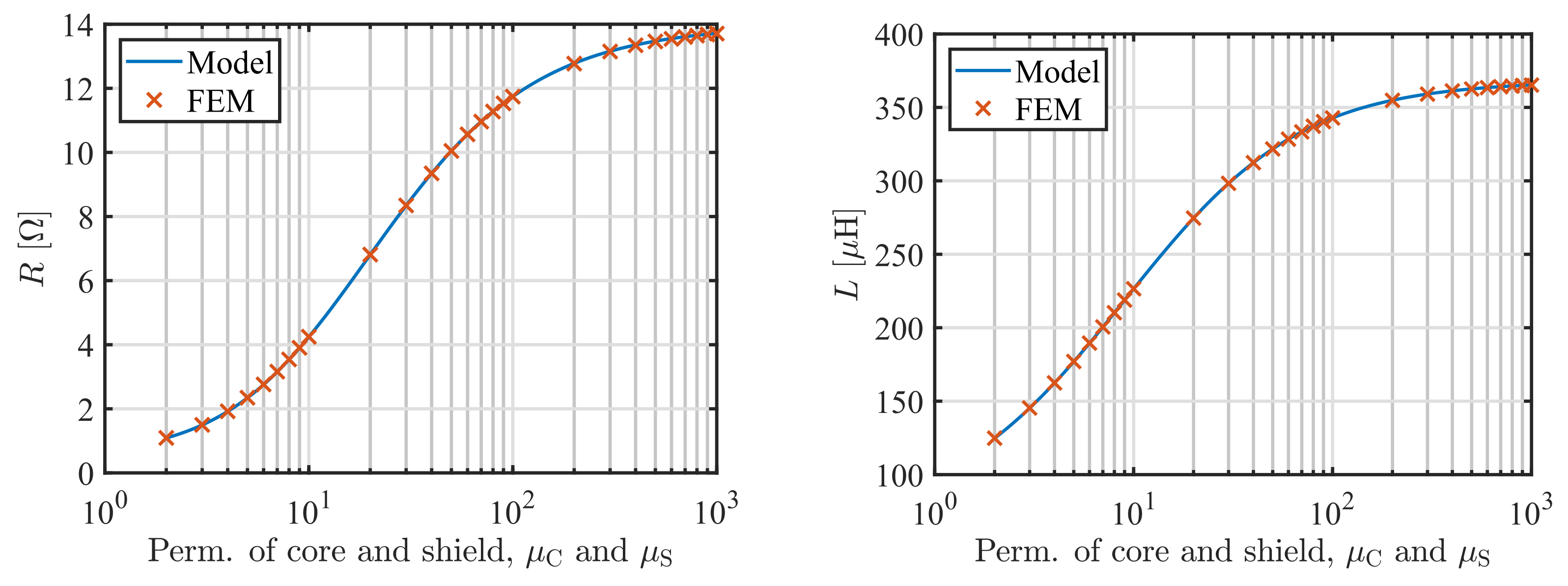
First, we calculated the impedance of the coil depending on the permeability of the core and shield for the plate with σ = 5   M S / m and μ r = 50 at 60 kHz, Figure 3. For the sake of simplicity, we assumed that μ C = μ S . There is practically no significant further change in the impedance of the sensor for the permeability above 500, which is a finding observed for other cored coils as well [17]. The relative discrepancy between the model and FEM results are bellow 0.07 % for the inductance and 0.23 % for the resistance. These discrepancies can be further reduced by increasing the density of the FEM mesh.
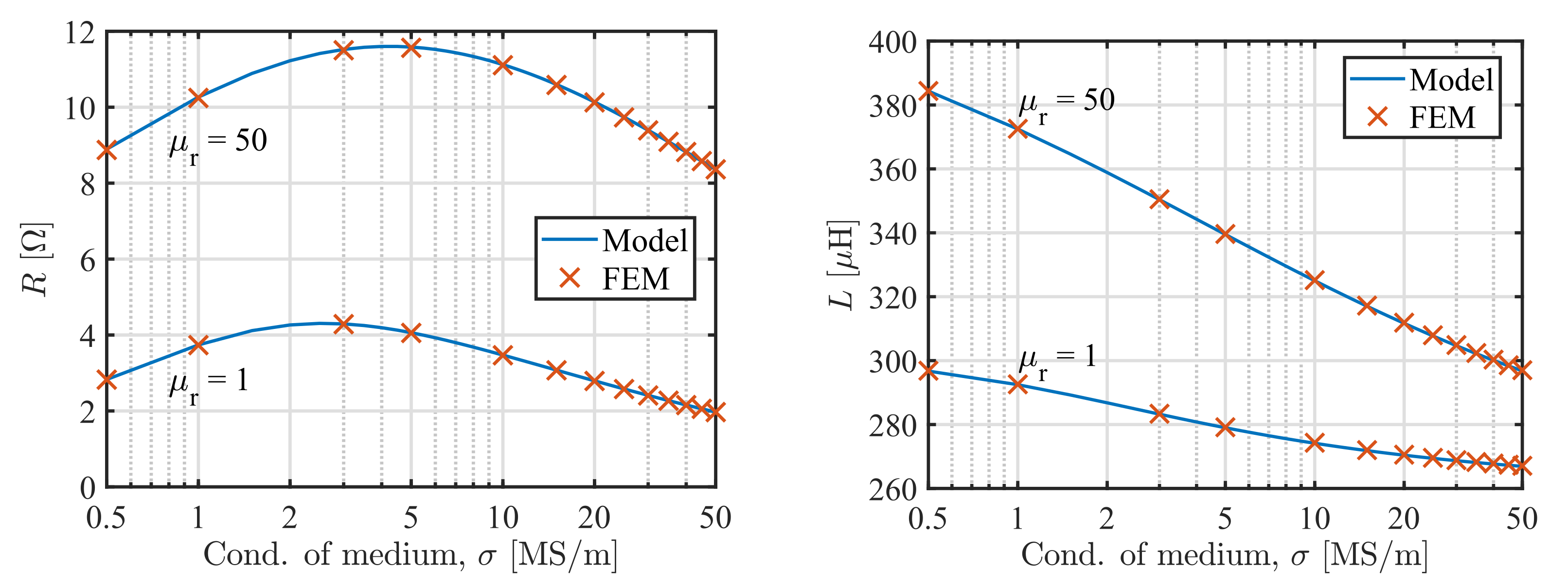
Second, we calculated the impedance of the coil depending on the conductivity σ of the plate for two values of its permeability μ r = 1 and μ r = 50 at 60 kHz, Figure 4. The core permeability μ C = 100 and the shield permeability μ S = 50 . Typical dependency of the coil impedance on the plate conductivity can be observed, including the maximum point of the resistance [17]. The relative discrepancy between the model and FEM results are bellow 0.07 % for the inductance and 0.25 % for the resistance.
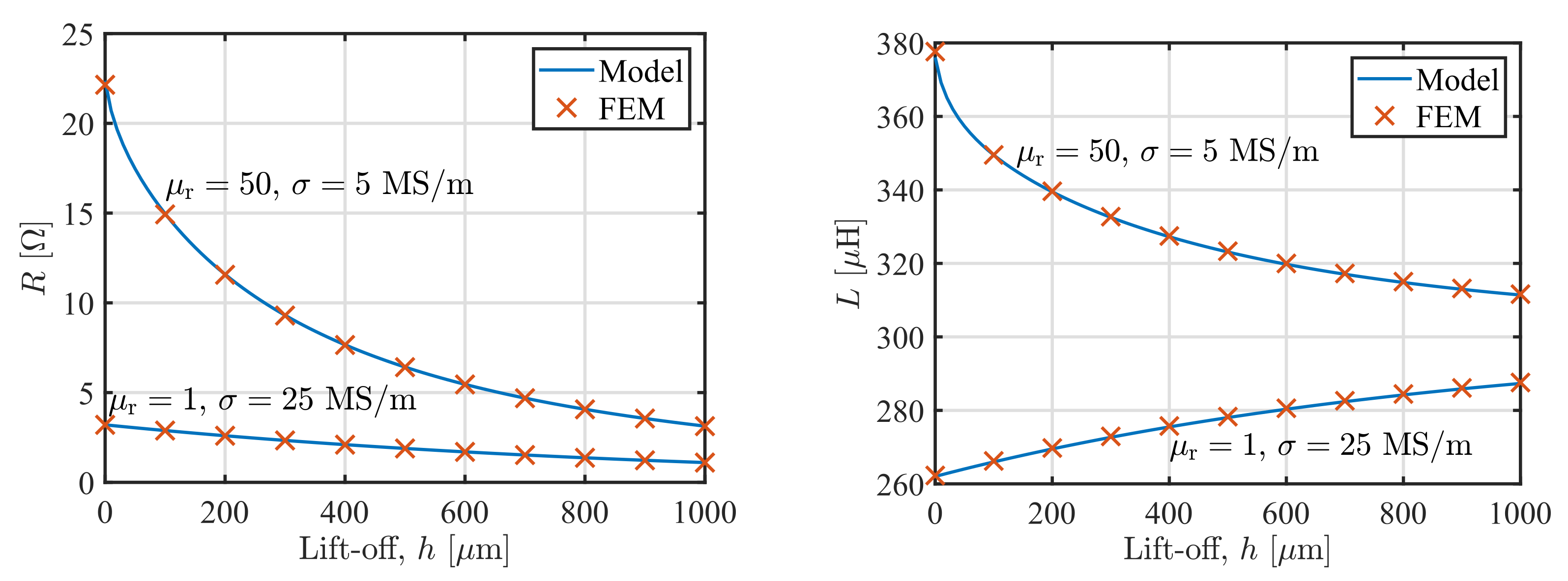
Finally, we calculated the impedance of the coil depending on the lift-off h of the sensor placed above either a nonmagnetic plate with μ r = 1 and σ = 25   M S / m (properties similar to an aluminum alloy), and a magnetic plate μ r = 50 and σ = 5 M S / m (properties similar to a carbon steel), Figure 5. The core permeability was μ C = 100 and the shield permeability μ S = 50 . Again, the relative discrepancy between the model and FEM results are bellow 0.07 % for the inductance and 0.25 % for the resistance. As expected, the resistance decreases with the lift-off increase for both plates, whereas the inductance in the case of the nonmagnetic plate increases with the lift-off, and decreases in the case of the magnetic plate.

5. Comparison with Experimental Results

We manufactured the sensor according to the geometry in Figure 1 and Figure 2. The sensor properties are given in Table 2. The impedance of the sensor in the air and above an aluminum plate was measured using the precision LCR meter HP 4284A in the frequency range from 5 kHz to 100 kHz and for lift-off values from 0 μ m to 1000 μ m in 100 μ m steps. The plate was made of aluminium alloy EN AW-6082 with a conductivity of 42.2 % IACS or 24.56   M S /m. The impedance of the coil Z is the sum of the coil impedance in air (without the plate) Z 0 = j ω L 0 , and the impedance change Δ Z = Δ R + j ω Δ L due to the proximity of the plate:
Z = j ω L 0 + Δ Z ,
where the resistance of the coil in air and the coil parasitic capacitance have been compensated for.
The inductance of the sensor in the air was calculated 1525.67   μ H , while the measured value was from 1524.48   μ H to 1526.38   μ H 
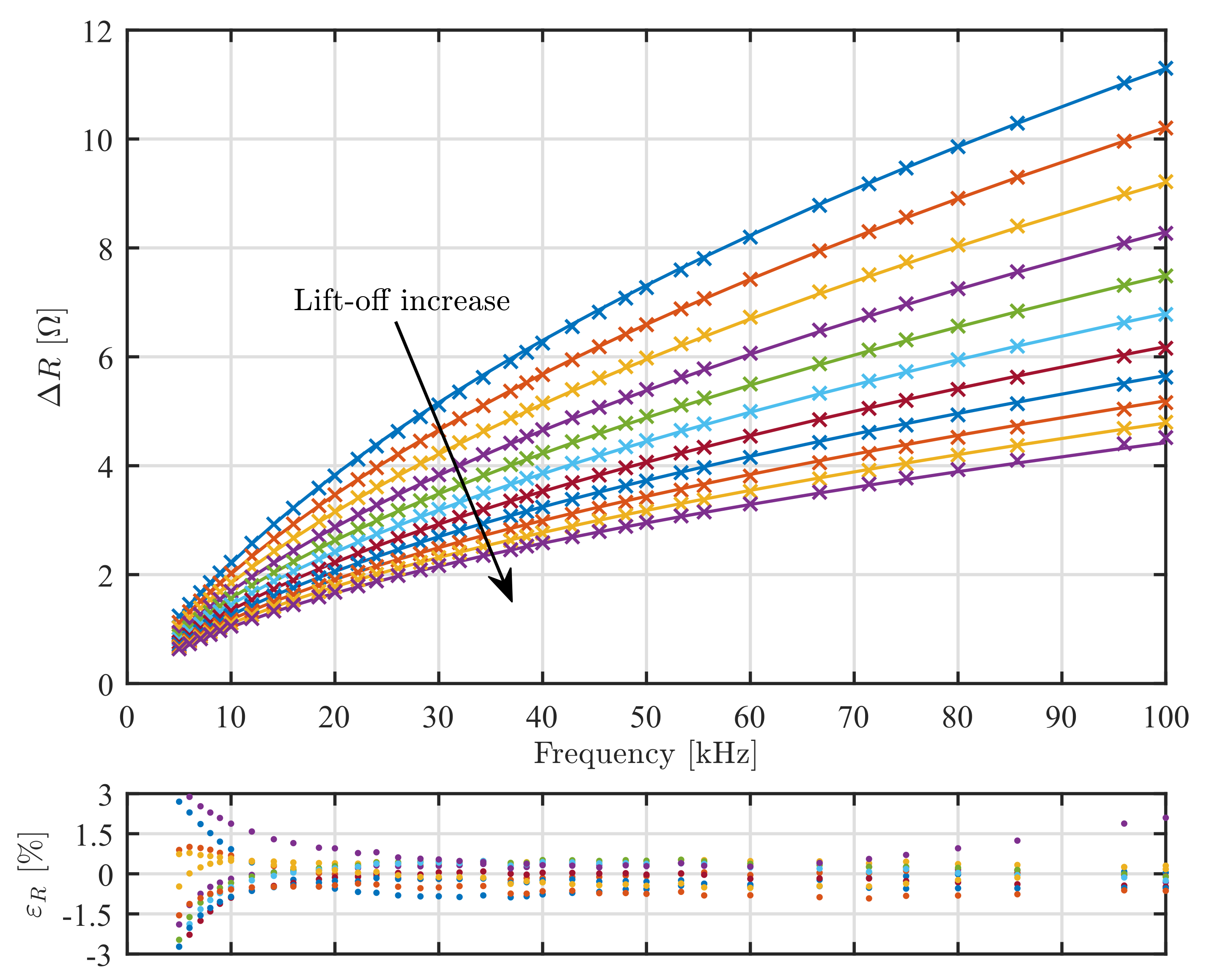
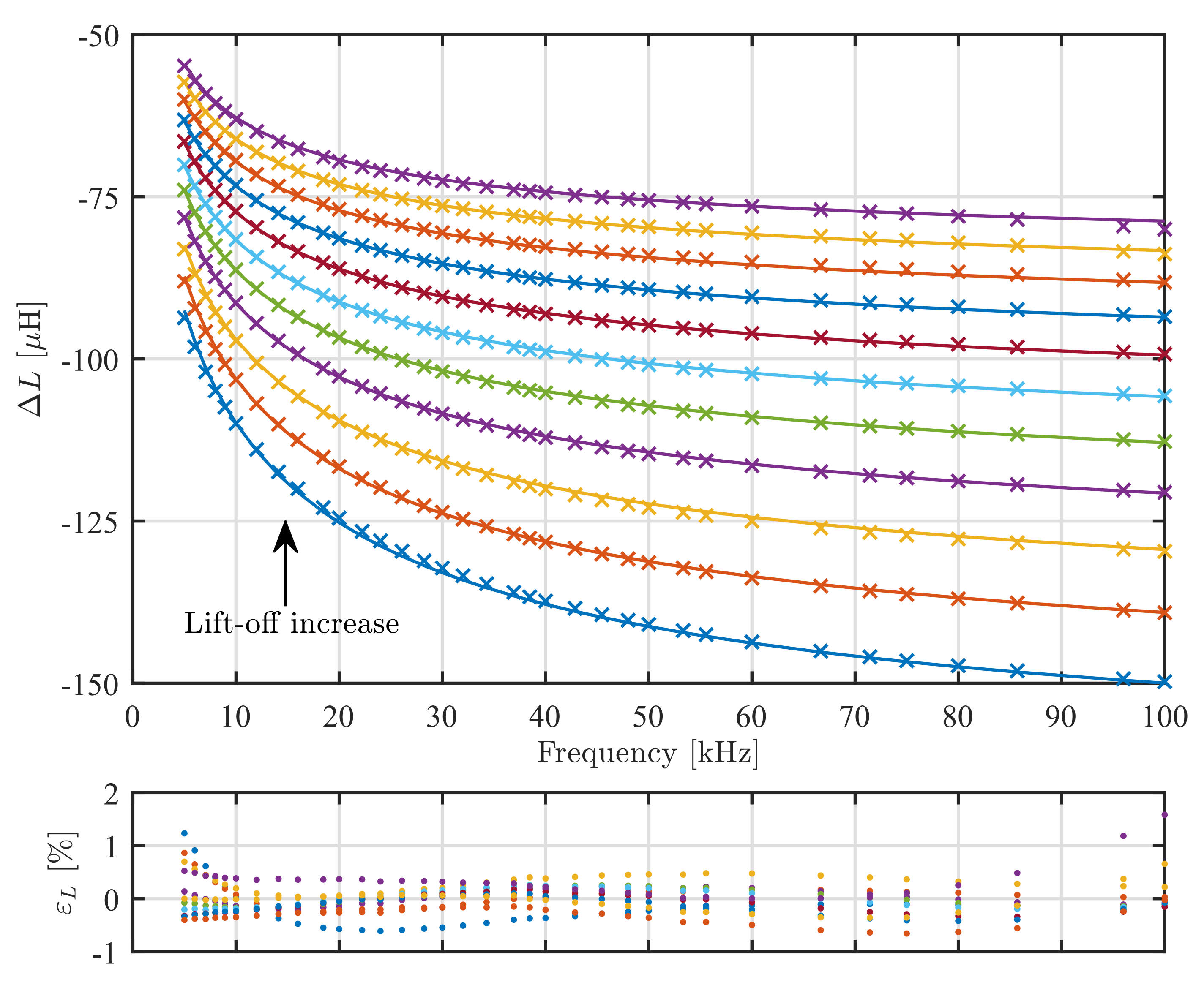
depending on the frequency. The impedance change obtained from the model and the experiment are shown in Figure 6 and Figure 7 for Δ R and Δ L , respectively. The model and experiment are in practically acceptable agreement with the relative error of Δ R within ± 3 % and Δ L within ± 1 % . These errors are comparable to the ones in other studies on eddy current sensor modeling. In practice, model-based measurements of conductivity and lift-off require calibration procedures with samples of known conductivity and lift-off if one wants to achieve measurement uncertainty better than the reported modeling errors would allow.

6. Sensitivity to Sensor Dimensions

The data in Table 2 was obtained by averaging and rounding to 0.01 mm the values measured using a Mitutoyo micrometer with resolution of 0.001 mm and accuracy of ± 2   μ m . We rounded the values because at a higher resolution, the measurement is affected by the applied pressure or measurement position along the measured object, e.g., the ferrite core was not a perfect cylinder at a resolution of 0.001 mm. We used purposefully overestimated measurement uncertainty of ± 0.01 mm to evaluate its effect on the sensor impedance. With that aim, we calculated the sensitivity of the sensor impedance to the sensor dimensions. Table 3 shows the relative changes of the inductance in the air L 0 and impedance change Δ R and Δ L (for plate with σ = 5   M S / m and μ r = 50 and lift-off 0 μ m ) if each of the nine sensor dimensions is independently varied within the interval of ± 0.01 mm. The core radius and the shield inner radius uncertainties have the most significant contribution to the impedance uncertainty. This means that the gap between the core and the shield must be precisely controlled during the sensor production.

7. Conclusions

The validity of the impedance model is corroborated by a practically negligible discrepancy in comparison with the FEM approach. We compared the model and FEM approach for a range of practical scenarios: changes of the impedance due to the variations in the core and shield permeabilities, dependence of the sensor impedance on the plate conductivity of magnetic and nonmagnetic plates and impedance dependence on the sensor lift-off above magnetic and nonmagnetic plates. The numerical implementation of the model is very fast in comparison to the FEM approach ( 0.7   s vs. 30 min), and this can be improved further if the intermediate results are reused for the next iteration. In comparison with the impedance measurement, the relative error better than 3 % in the frequency range from 5 kHz to 100 kHz confirms the applicability of the model for eddy current measurement of material properties and lift-off. The model can be extended easily to include multi-layered planar structures.

Author Contributions

Conceptualization, D.V. and M.K.; methodology, D.V. and I.R.; software, D.V., I.R. and D.Š.; validation, D.V., M.K. and I.R.; formal analysis, D.V. and D.Š.; resources, D.Š. and M.K.; writing—original draft preparation, D.V.; visualization, D.V.; supervision, D.V.; project administration, M.K.; funding acquisition, D.V. and M.K. All authors have read and agreed to the published version of the manuscript.

Funding

This research has been supported in part by the Croatian Science Foundation under the project UIP-2017-05-6948, MIMES—Models and Inverse Methods for Near Field Electromagnetic Sensors and in part through the European Regional Development Fund under grant KK.01.2.1.02.0129 (SmartEC).

Institutional Review Board Statement

Not applicable.

Informed Consent Statement

Not applicable.

Data Availability Statement

The data presented in this study are available on request from the corresponding author.

Conflicts of Interest

The authors declare no conflict of interest. The funders had no role in the design of the study; in the collection, analyses or interpretation of data; in the writing of the manuscript or in the decision to publish the results.

Appendix A. Interface Relations for Horizontal Boundaries

The following integrals involving the Bessel functions will be very useful:
t X ν a t Ψ ν b t d t = ± t a 2 b 2 a X ν ± 1 a t Ψ ν b t b X ν a t Ψ ν ± 1 b t ,
t X 0 a t Ψ 0 a t d t = t 2 2 X 0 a t Ψ 0 a t + X 1 a t Ψ 1 a t ,
where X and Ψ are any two cylinder functions.

Appendix A.1. Interface z = LS

Because of the piecewise definition of the radial part of the potential, the following equations are obtained from the continuity of B z according to (37):
J 0 α ¯ r exp α L S C ̲ 1 = = J 0 p ¯ r , 0 r r S 1 , R 0 , 22 p ¯ r , r S 1 r r S 2 , R 0 , 23 p ¯ r , r S 2 r R , exp p L S C ̲ 2 + exp p L S D ̲ 2 .
If both sides of (A3) are multiplied from the left by the basis function,
X p ̲ r = J 0 p ̲ r , 0 r r S 1 , 1 μ S R 0 , 22 p ̲ r , r S 1 r r S 2 , R 0 , 23 p ̲ r , r S 2 r R ,
and then integrated from 0 to R, we obtain
E exp α L S C ̲ 1 = K exp p L S C ̲ 2 + K exp p L S D ̲ 2 ,
where elements of matrices E = e i k and K = k i k are
e i k = 0 r S 1 r J 0 p i r J 0 α k r d r + r S 1 r S 2 r 1 μ S R 0 , 22 p i r J 0 α k r d r + r S 2 R r R 0 , 23 p i r J 0 α k r d r = = 1 p i 2 α k 2 1 1 μ S p i r S 1 J 1 p i r S 1 J 0 α k r S 1 p i r S 2 R 1 , 23 p i r S 2 J 0 α k r S 2 ,
k i k = 0 r S 1 r J 0 p i r J 0 p k r d r + + r S 1 r S 2 r 1 μ S R 0 , 22 p i r R 0 , 22 p k r d r + r S 2 R r R 0 , 23 p i r R 0 , 23 p k r d r = = 0 , for i k R 2 2 R 0 , 23 2 p i R + r S 2 2 2 μ S 1 R 0 , 23 2 p i r S 2 r S 2 2 2 1 1 μ S R 1 , 23 2 p i r S 2 r S 1 2 2 μ S 1 J 0 2 p i r S 1 + r S 1 2 2 1 1 μ S J 1 2 p i r S 1 , for i = k ,
where p i and α k are elements of the vectors p ̲ and α ¯ , E is full, and K is diagonal.
Continuity of H r according to (38) results in the following:
J 1 α ¯ r exp α L S C ̲ 1 = = J 1 p ¯ r , 0 r r S 1 , 1 μ S R 1 , 22 p ¯ r , r S 1 r r S 2 , R 1 , 23 p ¯ r , r S 2 r R , exp p L S C ̲ 2 exp p L S D ̲ 2 ,
X p ̲ r = J 1 p ̲ r , 0 r r S 1 , R 1 , 22 p ̲ r , r S 1 r r S 2 , R 1 , 23 p ̲ r , r S 2 r R ,
F exp α L S C ̲ 1 = K exp p L S C ̲ 2 K exp p L S D ̲ 2 ,
f i k = 1 p i 2 α k 2 μ S 1 p i r S 1 J 0 p i r S 1 J 1 α k r S 1 p i r S 2 R 0 , 23 p i r S 2 J 1 α k r S 2 .

Appendix A.2. Interface z = LC

Continuity of B z according to (37) results in the following:
J 0 p ¯ r , 0 r r S 1 , R 0 , 22 p ¯ r , r S 1 r r S 2 , R 0 , 23 p ¯ r , r S 2 r R , exp p L C C ̲ 2 + exp p L C D ̲ 2 = = J 0 q ¯ r , 0 r r C , R 0 , 32 q ¯ r , r C r r S 1 , R 0 , 33 q ¯ r , r S 1 r r S 2 , R 0 , 34 q ¯ r , r S 2 r R , exp q L C C ̲ 3 + exp q L C D ̲ 3 ,
K exp p L C C ̲ 2 + K exp p L C D ̲ 2 = W exp q L C C ̲ 3 + W exp q L C D ̲ 3 ,
w i k = 1 p i 2 q k 2 1 1 μ C p i r C J 1 p i r C J 0 q k r C .
The basis function X p ̲ r is given by (A4).
Continuity of H r according to (38) results in the following:
J 1 p ¯ r , 0 r r S 1 , 1 μ S R 1 , 22 p ¯ r , r S 1 r r S 2 , R 1 , 23 p ¯ r , r S 2 r R , exp p L C C ̲ 2 exp p L C D ̲ 2 = = 1 μ C J 1 q ¯ r , 0 r r C , R 1 , 32 q ¯ r , r C r r S 1 , 1 μ S R 1 , 33 q ¯ r , r S 1 r r S 2 , R 1 , 34 q ¯ r , r S 2 r R , exp q L C C ̲ 3 exp q L C D ̲ 3 ,
K exp p L C C ̲ 2 K exp p L C D ̲ 2 = L exp q L C C ̲ 3 L exp q L C D ̲ 3 ,
l i k = 1 p i 2 q k 2 1 1 μ C p i r C J 0 p i r C J 1 q k r C .
In this case, the basis function X p ̲ r is given by (A9).

Appendix A.3. Interface z = z0

Continuity of B z according to (37) results in the following:
exp q z 0 C ̲ 3 + exp q z 0 D ̲ 3 = exp q z 0 C ̲ 4 + exp q z 0 D ̲ 4 .
Continuity of H r according to (38) results in the following:
1 μ C J 1 q ¯ r , 0 r r C , R 1 , 32 q ¯ r , r C r r S 1 , 1 μ S R 1 , 33 q ¯ r , r S 1 r r S 2 , R 1 , 34 q ¯ r , r S 2 r R , exp q z 0 C ̲ 3 exp q z 0 D ̲ 3 = 1 μ C J 1 q ¯ r , 0 r r C , R 1 , 42 q ¯ r , r C r r S 1 , 1 μ S R 1 , 43 q ¯ r , r S 1 r r S 2 , R 1 , 44 q ¯ r , r S 2 r R , exp q z 0 C ̲ 4 exp q z 0 D ̲ 4 + μ 0 I δ r r 0 ,
X q ̲ r = J 1 q ̲ r , 0 r r C , R 1 , 32 q ̲ r , r C r r S 1 , R 1 , 33 q ̲ r , r S 1 r r S 2 , R 1 , 34 q ̲ r , r S 2 r R ,
exp q z 0 C ̲ 3 exp q z 0 D ̲ 3 =   = exp q z 0 C ̲ 4 exp q z 0 D ̲ 4 + μ 0 I S 1 r 0 R 1 , 32 q ̲ r 0 ,
s i k = 0 , for i k R 2 2 R 0 , 34 2 q i R + r C 2 2 1 μ C 1 1 μ C J 0 2 q i r C r C 2 2 1 1 μ C J 1 2 q i r C r S 1 2 2 1 μ S 1 1 μ S R 0 , 33 2 q i r S 1 + r S 1 2 2 1 1 μ S R 1 , 33 2 q i r S 1 + + r S 2 2 2 μ S 1 R 0 , 34 2 q i r S 2 r S 2 2 2 1 1 μ S R 1 , 34 2 q i r S 2 , for i = k .

Appendix A.4. Interface z = 0

Continuity of B z according to (37) results in the following:
J 0 q ¯ r , 0 r r C , R 0 , 42 q ¯ r , r C r r S 1 , R 0 , 43 q ¯ r , r S 1 r r S 2 , R 0 , 44 q ¯ r , r S 2 r R , C ̲ 4 + D ̲ 4 = J 0 α ¯ r C ̲ 5 + D ̲ 5 ,
X q ̲ r = 1 μ C J 0 q ̲ r , 0 r r C , R 0 , 32 q ̲ r , r C r r S 1 , 1 μ S R 0 , 33 q ̲ r , r S 1 r r S 2 , R 0 , 34 q ̲ r , r S 2 r R ,
S C ̲ 4 + S D ̲ 4 = V C ̲ 5 + V D ̲ 5 ,
v i k = 1 q i 2 α k 2 1 1 μ C q i r C J 1 q i r C J 0 α k r C + + 1 1 μ S q i r S 1 R 1 , 43 q i r S 1 J 0 α k r S 1 1 1 μ S q i r S 2 R 1 , 44 q i r S 2 J 0 α k r S 2 .
Continuity of H r according to (38) results in the following:
1 μ C J 1 q ¯ r , 0 r r C , R 1 , 42 q ¯ r , r C r r S 1 , 1 μ S R 1 , 43 q ¯ r , r S 1 r r S 2 , R 1 , 44 q ¯ r , r S 2 r R , C ̲ 4 D ̲ 4 = J 1 α ¯ r C ̲ 5 D ̲ 5 ,
S C ̲ 4 S D ̲ 4 = U C ̲ 5 U D ̲ 5 ,
u i k = 1 q i 2 α k 2 1 1 μ C q i r C J 0 q i r C J 1 α k r C + + 1 1 μ S q i r S 1 R 0 , 43 q i r S 1 J 1 α k r S 1 μ S 1 q i r S 2 R 0 , 44 q i r S 2 J 1 α k r S 2 .
The basis function X q ̲ r is given by (A20).

Appendix A.5. Interface z = −h

Continuity of B z and H r according to (37) and (38) result in the following:
exp α h C ̲ 5 + exp α h D ̲ 5 = α β 1 exp β h D ̲ 6 ,
exp α h C ̲ 5 exp α h D ̲ 5 = 1 μ r exp β h D ̲ 6 .

References

  1. García-Martín, J.; Gómez-Gil, J.; Vázquez-Sánchez, E. Non-destructive techniques based on eddy current testing. Sensors 2011, 11, 2525–2565. [Google Scholar] [CrossRef] [PubMed] [Green Version]
  2. AbdAlla, A.N.; Faraj, M.A.; Samsuri, F.; Rifai, D.; Ali, K.; Al-Douri, Y. Challenges in improving the performance of eddy current testing: Review. Meas. Control 2019, 52, 46–64. [Google Scholar] [CrossRef] [Green Version]
  3. Vasić, D.; Bilas, V.; Ambruš, D. Pulsed eddy-current nondestructive testing of ferromagnetic tubes. IEEE Trans. Instrum. Meas. 2004, 53, 1289–1294. [Google Scholar] [CrossRef]
  4. Reyno, T.; Underhill, P.R.; Krause, T.W.; Marsden, C.; Wowk, D. Surface Profiling and Core Evaluation of Aluminum Honeycomb Sandwich Aircraft Panels Using Multi-Frequency Eddy Current Testing. Sensors 2017, 17, 2114. [Google Scholar] [CrossRef] [Green Version]
  5. Zhang, W.; Shi, Y.; Li, Y.; Luo, Q. A study of quantifying thickness of ferromagnetic pipes based on remote field eddy current testing. Sensors 2018, 18, 2769. [Google Scholar] [CrossRef] [PubMed] [Green Version]
  6. Meng, X.; Lu, M.; Yin, W.; Bennecer, A.; Kirk, K.J. Evaluation of Coating Thickness Using Lift-Off Insensitivity of Eddy Current Sensor. Sensors 2021, 21, 419. [Google Scholar] [CrossRef]
  7. Lu, M.; Meng, X.; Huang, R.; Chen, L.; Peyton, A.; Yin, W.; Qu, Z. Thickness measurement of circular metallic film using single-frequency eddy current sensor. NDT & E Int. 2021, 119, 102420. [Google Scholar] [CrossRef]
  8. Zergoug, M.; Lebaili, S.; Boudjellal, H.; Benchaala, A. Relation between mechanical microhardness and impedance variations in eddy current testing. NDT & E Int. 2004, 37, 65–72. [Google Scholar] [CrossRef]
  9. Lu, M.; Xu, H.; Zhu, W.; Yin, L.; Zhao, Q.; Peyton, A.; Yin, W. Conductivity lift-off invariance and measurement of permeability of ferrite metallic plates. NDT & E Int. 2018, 95, 36–44. [Google Scholar] [CrossRef]
  10. Adewale, I.; Tian, G. Decoupling the influence of permeability and conductivity in pulsed eddy-current measurement. IEEE Trans. Magn. 2013, 49, 1119–1127. [Google Scholar] [CrossRef]
  11. Sophian, A.; Tian, G.Y.; Taylor, D.; Rudlin, J. A feature extraction technique based on principal component analysis for pulsed Eddy current NDT. NDT & E Int. 2003, 36, 37–41. [Google Scholar] [CrossRef]
  12. Bernieri, A.; Ferrigno, L.; Laracca, M.; Molinara, M. Crack Shape Reconstruction in Eddy Current Testing Using Machine Learning Systems for Regression. IEEE Trans. Instrum. Meas. 2008, 57, 1958–1968. [Google Scholar] [CrossRef]
  13. Yuan, F.; Yu, Y.; Wang, W.; Xue, K.; Tian, G. Pulsed eddy current array design and electromagnetic imaging for defects detection in metallic materials. Nondestruct. Test. Eval. 2021, 1–19. [Google Scholar] [CrossRef]
  14. Sophian, A.; Tian, G.; Fan, M. Pulsed Eddy Current Non-destructive Testing and Evaluation: A Review. Chin. J. Mech. Eng. 2017, 30, 500–514. [Google Scholar] [CrossRef] [Green Version]
  15. Skarlatos, A.; Pichenot, G.; Lesselier, D.; Lambert, M.; Duchene, B. Electromagnetic modeling of a damaged ferromagnetic metal tube by a volume integral equation formulation. IEEE Trans. Magn. 2008, 44, 623–632. [Google Scholar] [CrossRef]
  16. Dodd, C.V.; Deeds, W.E. Analytical solutions to eddy-current probe-coil problems. J. Appl. Phys. 1968, 39, 2829–2838. [Google Scholar] [CrossRef] [Green Version]
  17. Theodoulidis, T.P.; Kriezis, E.E. Eddy Current Canonical Problems (with Applications to Nondestructive Evaluation); Tech Science Press: Forsyth, GA, USA, 2006. [Google Scholar]
  18. Theodoulidis, T.P. Model of ferrite-cored probes for eddy current nondestructive evaluation. J. Appl. Phys. 2003, 93, 3071–3078. [Google Scholar] [CrossRef]
  19. Lu, Y.; Bowler, J.R.; Theodoulidis, T.P. An analytical model of a ferrite-cored inductor used as an eddy current probe. J. Appl. Phys. 2012, 111, 103907. [Google Scholar] [CrossRef]
  20. Bayani, H.; Theodoulidis, T.; Sasada, I. Application of Eigenfunction Expansions to Eddy Current NDE: A model of Cup-Cored Probes. Electromagn. Nondestruct. Eval. (X) 2007, 28, 57–64. [Google Scholar]
  21. Sakkaki, F.; Bayani, H. Solution to the problem of E-cored coil above a layered half-space using the method of truncated region eigenfunction expansion. J. Appl. Phys. 2012, 111, 2–5. [Google Scholar] [CrossRef]
  22. Tytko, G.; Dziczkowski, L. I-cored Coil Probe Located above a Conductive Plate with a Surface Hole. Meas. Sci. Rev. 2018, 18, 7–12. [Google Scholar] [CrossRef] [Green Version]
  23. Tytko, G.; Dziczkowski, L. An analytical model of an I-cored coil located above a conductive material with a hole. Eur. Phys. J. Appl. Phys. 2018, 82, 21001. [Google Scholar] [CrossRef]
  24. Tytko, G.; Dziczkowski, L. Calculation of the Impedance of an E-cored Coil Placed above a Conductive Material with a Surface Hole. Meas. Sci. Rev. 2019, 19, 43–47. [Google Scholar] [CrossRef] [Green Version]
  25. Zhu, Y.; Chen, B.; Luo, Y.; Zhu, R. Inductance calculations for coaxial iron-core coils shielded by cylindrical screens of high permeability. IET Electr. Power Appl. 2019, 13, 742–749. [Google Scholar] [CrossRef]
  26. ISO 21968:2019; Non-Magnetic Metallic Coatings on Metallic and Non-Metallic Basis Materials—Measurement of Coating Thickness—Phase-Sensitive Eddy-Current Method. International Organization for Standardization: Geneva, Switzerland, 2019.
  27. Anderson, N.; Björck, Å. A new high order method of regula falsi type for computing a root of an equation. BIT Numer. Math. 1973, 13, 253–264. [Google Scholar] [CrossRef]
  28. Abramowitz, M.; Stegun, I.A. Handbook of Mahematical Functions (Entries 11.1.7, 12.1.19–20), 10th ed.; National Bureau of Standards: Washington, DC, USA, 1972.
  29. Meeker, D.C. Finite Element Method Magnetics—FEMM, Version 4.2; Available online: https://www.femm.info (accessed on 28 October 2021).
Figure 1. The sensor above the plate. The shield is shown as transparent/cut to show the sensor inside.
Sensors 22 00326 g001
Figure 2. A ferrite-cored coil screened with a ferrite shield above magnetic and conductive half space. A filamentary coil is also shown. For better clarity, the subregions of a region are indicated by colors with the same hue value but different lightness. In the case of the filamentary coil, region C is not present and the boundary between regions 3 and 4 is at z = z 0 .
Sensors 22 00326 g002
Figure 3. Comparison of the model predictions and results of the FEM study for resistance R (left) and inductance L (right) of the sensor depending on the permeability of the core μ C and shield μ S assuming that μ C = μ S . The plate has σ = 5   M S / m and μ r = 50 , and the frequency is 60 kHz.
Sensors 22 00326 g003
Figure 4. Comparison of the model predictions and results of the FEM study for resistance R (left) and inductance L (right) of the sensor at 60 kHz depending on the conductivity of the medium σ for two cases of the permeability of the plate μ r = 1 and μ r = 50 . The core has μ C = 100 and the shield μ S = 50 .
Sensors 22 00326 g004
Figure 5. Comparison of the model predictions and results of the FEM study for resistance R (left) and inductance L (right) of the sensor at 60 kHz depending on the lift-off h for two plates: μ r = 1 and σ = 25   M S / m , and μ r = 50 and σ = 5   M S / m . The core has μ C = 100 and the shield μ S = 50 .
Sensors 22 00326 g005
Figure 6. Real part Δ R of impedance change Δ Z . Full lines are modeling results and crosses are measured values. The top curve is for lift-off 0 μ m and the bottom curve for 1000 μ m . Other curves are in 100 μ m increments. The graph bellow shows error ε R of individual measurement data points relative to the model prediction.
Sensors 22 00326 g006
Figure 7. Imaginary part Δ L of impedance change Δ Z . Full lines are modeling results and crosses are measured values. The bottom curve is for lift-off 0 μ m and the top curve for 1000 μ m . Other curves are in 100 μ m increments. The graph bellow shows error ε L of individual measurement data points relative to the model prediction.
Sensors 22 00326 g007
Table 1. Properties of the sensor used in the numerical studies.
Coil
Inner radius r T 1 2.50 mm
Outer radius r T 2 3.15 mm
Bottom position z T 1 2.00 mm
Top position z T 2 4.00 mm
Lift-offh 0.20 mm
Number of turns N TX 128
Core
Radius r C 1.75 mm
Height L C 6.00 mm
Rel. permeability μ C see the text
Shield
Inner radius r S 1 3.65 mm
Outer radius r S 2 6.05 mm
Height L S 15.50 mm
Rel. permeability μ S see the text
Table 2. Properties of the sensor prototype.
Coil
Inner radius r T 1 5.00 mm
Outer radius r T 2 5.09 mm
Bottom position z T 1 2.45 mm
Top position z T 2 17.45 mm
Number of turns N TX 125
Core
Radius r C 4.98 mm
Height L C 20.03 mm
Material HF 70
Rel. permeability μ C 1500
Shield
Inner radius r S 1 6.45 mm
Outer radius r S 2 12.92 mm
Height L S 28.29 mm
Material 4 W 620
Rel. permeability μ S 620
Table 3. Relative uncertainty of sensor impedance in the case of ± 0.01 mm uncertainty in sensor dimensions. The plate has σ   =   5   M S / m and μ r = 50 , lift-off is 0 μ m and the frequency is 60 kHz.
Parameter ValueUncertainty Relative Uncertainty of
L 0 Δ R Δ L
Coil
Inner radius r T 1 5.00 mm ± 0.01 mm ± 2.6   ppm ± 2.6   ppm ± 2.6   ppm
Outer radius r T 2 5.09 mm ± 0.01 mm ± 2.5   ppm ± 2.4   ppm ± 2.4   ppm
Bottom position z T 1 2.45 mm ± 0.01 mm ± 542   ppm 872   ppm 874   ppm
Top position z T 2 17.45 mm ± 0.01 mm 482   ppm 856   ppm 856   ppm
Core
Radius r C 4.98 mm ± 0.01 mm ± 6776   ppm ± 5632   ppm ± 7646   ppm
Height L C 20.03 mm ± 0.01 mm ± 724   ppm ± 879   ppm ± 788   ppm
Shield
Inner radius r S 1 6.45 mm ± 0.01 mm 4858   ppm 4030   ppm 6933   ppm
Outer radius r S 2 12.92 mm ± 0.01 mm ± 8.9   ppm ± 30.4   ppm ± 65   ppm
Height L S 28.29 mm ± 0.01 mm ± 0.2   ppm ± 0.2   ppm ± 0.6   ppm
Publisher’s Note: MDPI stays neutral with regard to jurisdictional claims in published maps and institutional affiliations.

