
Co-Channel Interference Suppression for LTE Passive Radar Based on Spatial Feature Cognition


Abstract
:1. Introduction
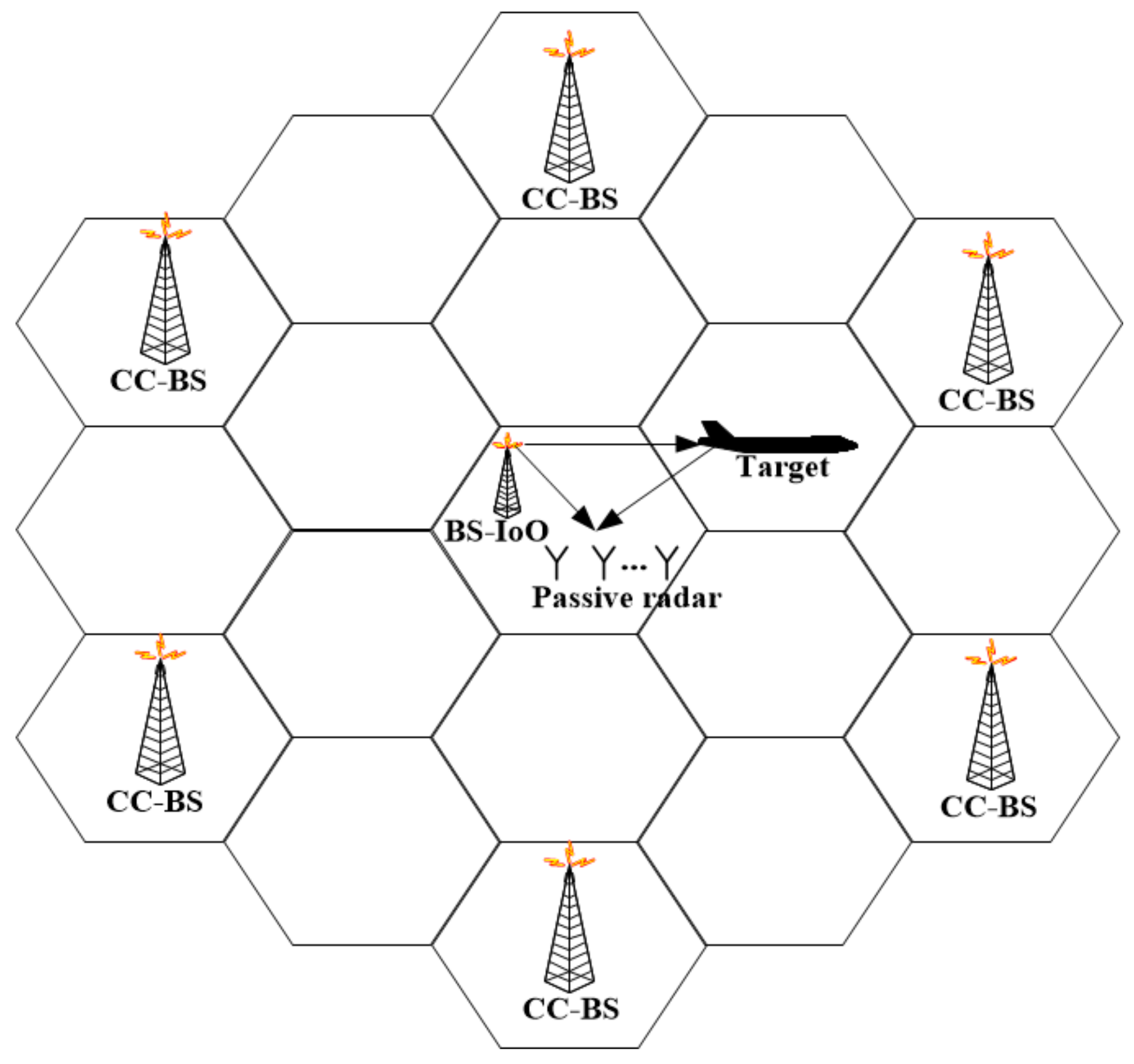
2. Signal Model
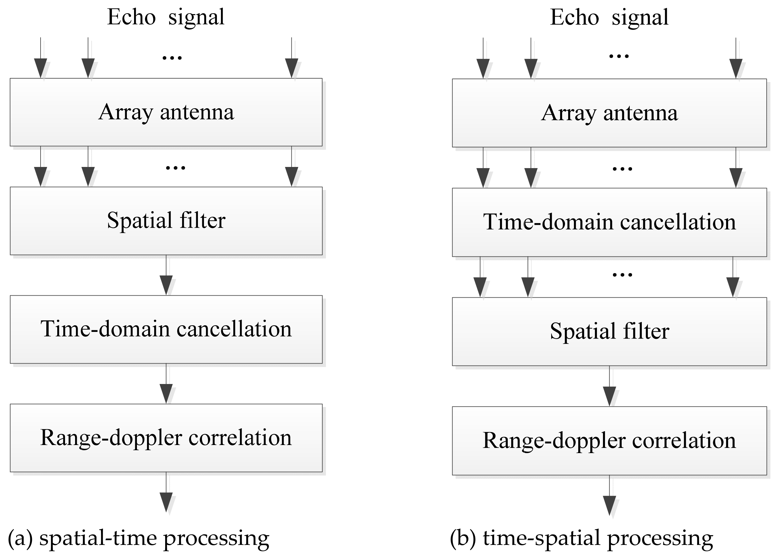
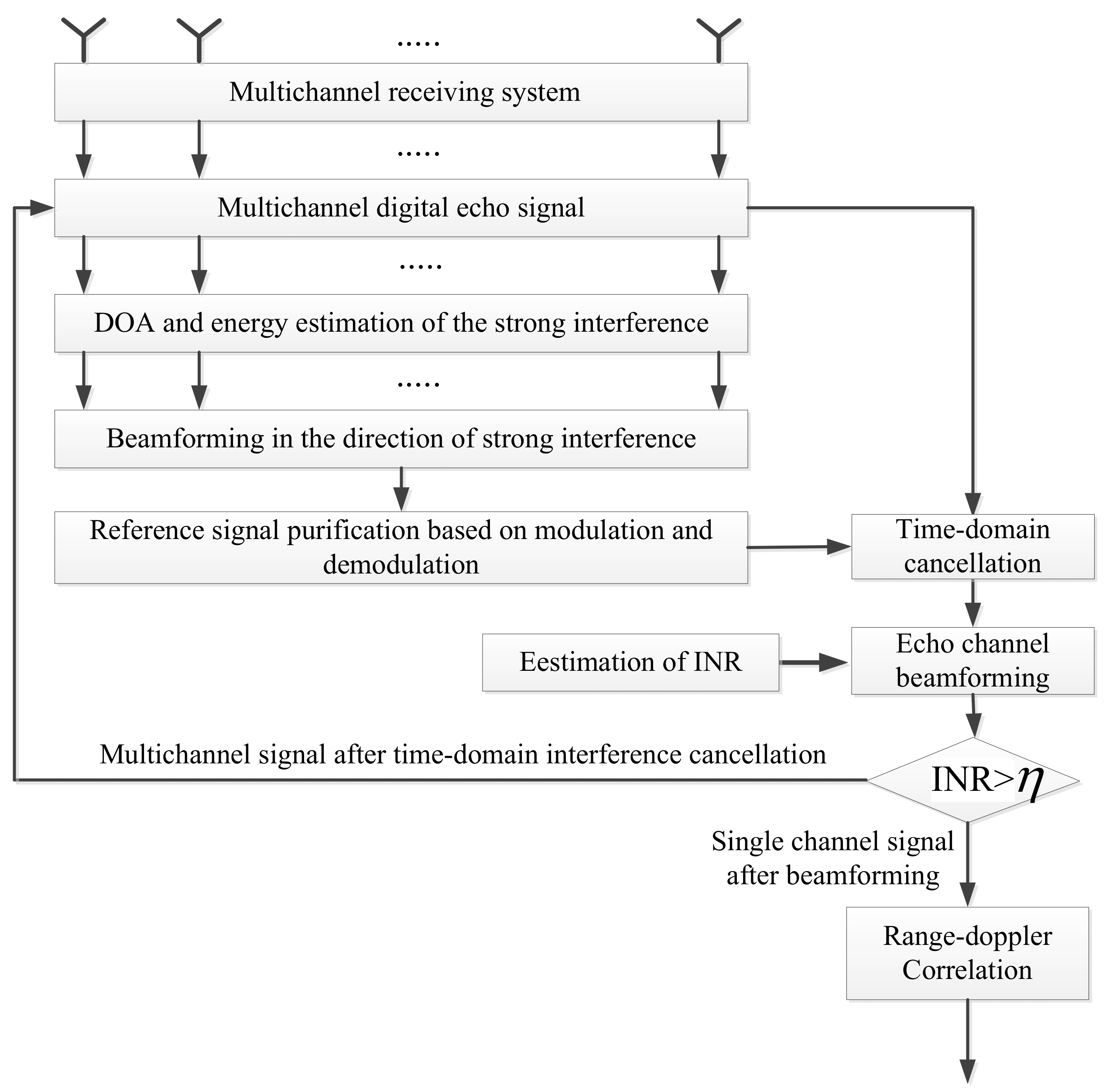
3. Algorithm Description
- (1)
- DOA and energy estimation of the strong interference:
- (2)
- Beamforming in the direction of strong interference:
- (3)
- Purification of the direct signal based on demodulation and reconstruction:
- (4)
- Time-domain interference cancellation:
- (5)
- Spatial beamforming in the surveillance region:
- (6)
- Evaluation of interference suppression effect:
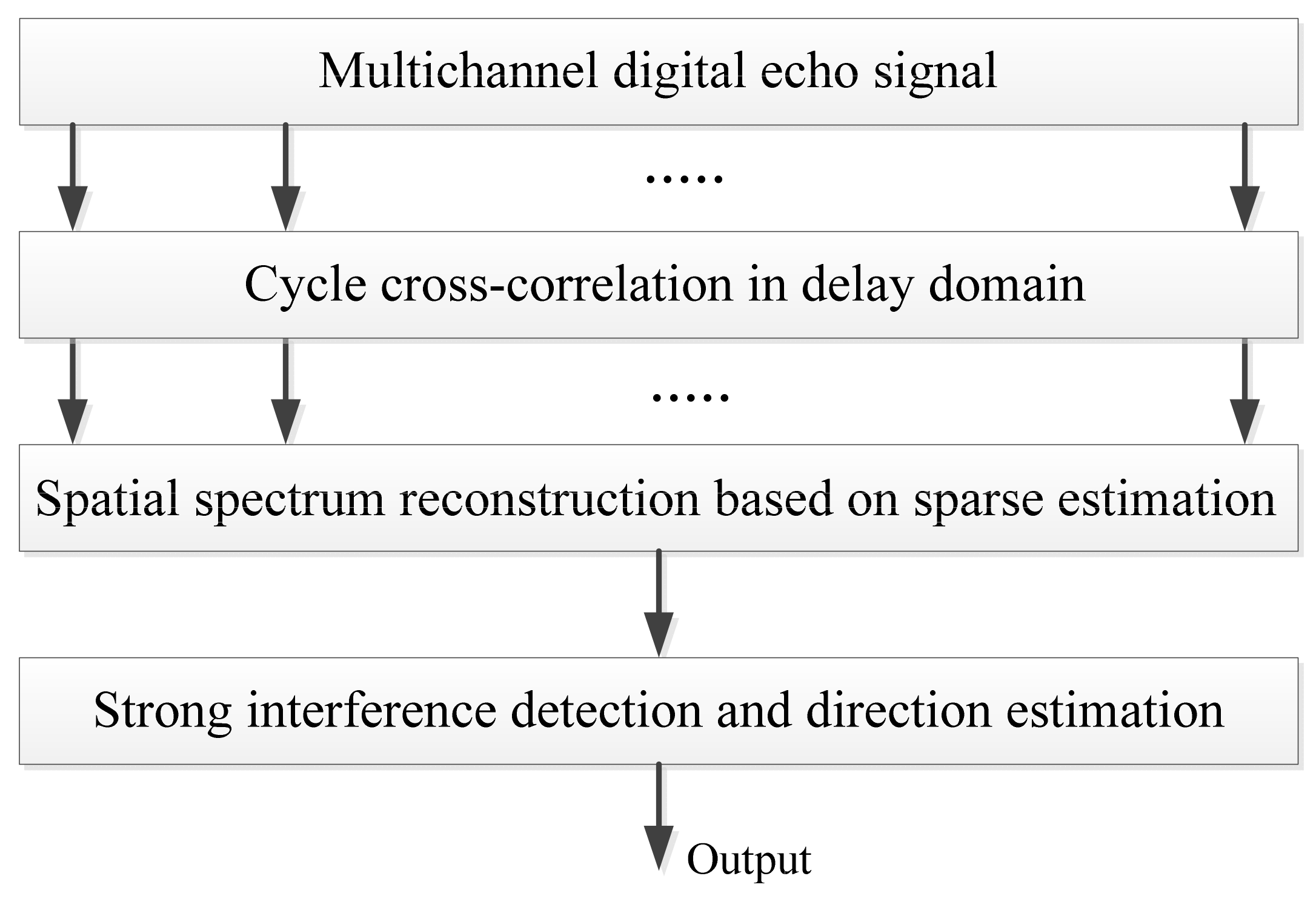
3.1. Direction Finding of the Interference based on the Cyclostationary Characteristics of the OFDM Signal and the Sparse Reconstruction Technique
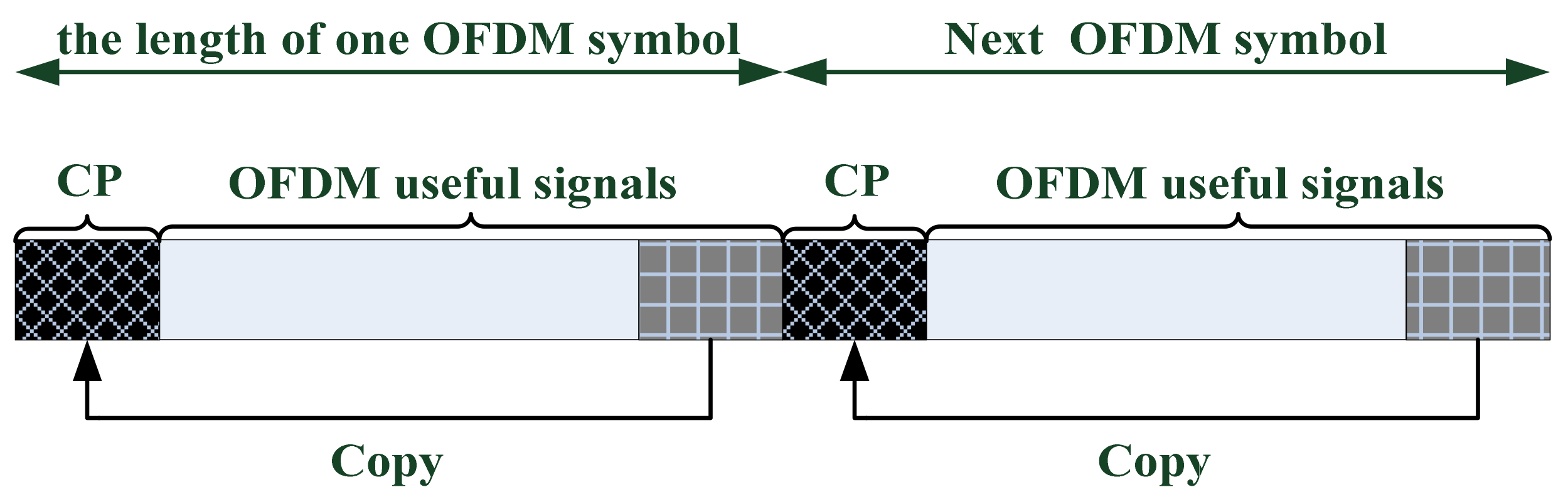
3.1.1. Cycle Cross-Correlation (CCC) in Delay Domain
3.1.2. Spatial Spectrum Reconstruction of the Interference Signal based on the Sparse Estimation
3.2. Co-Channel Interference Suppression based on Spatial Feature Cognition
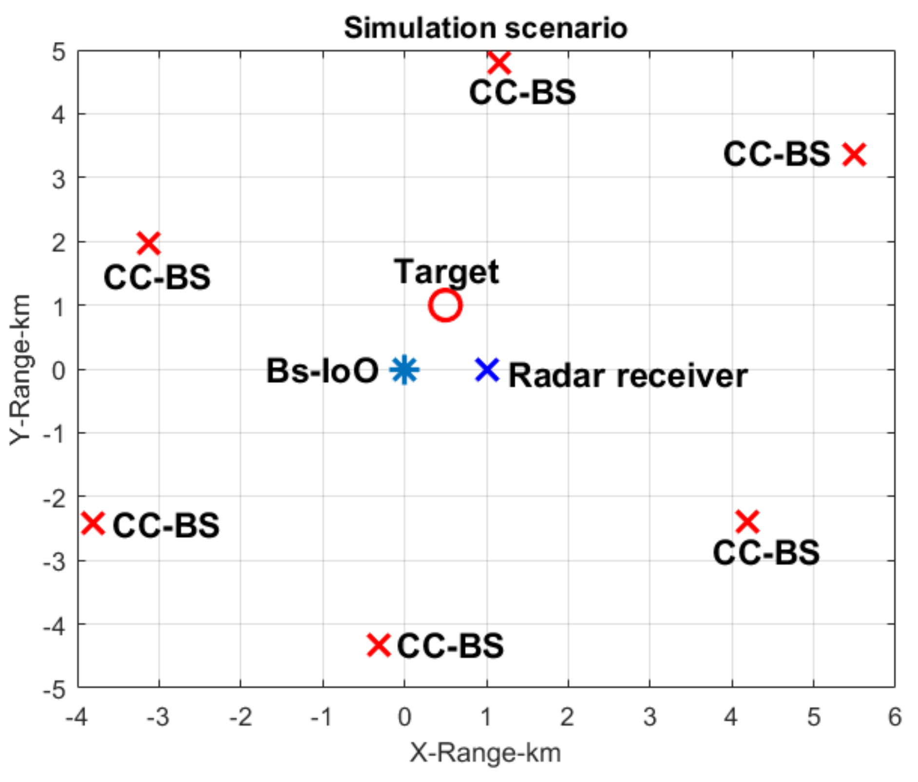
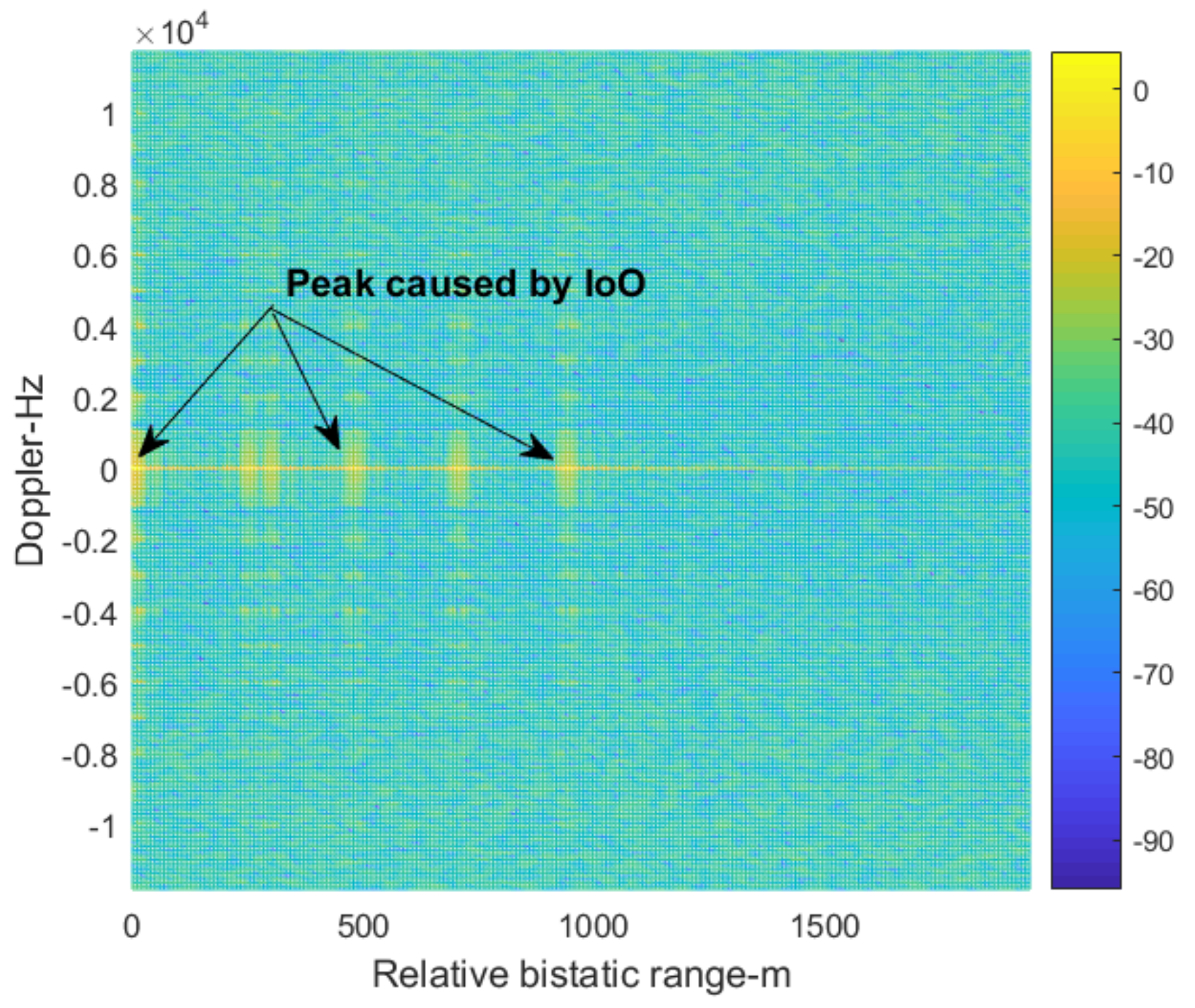
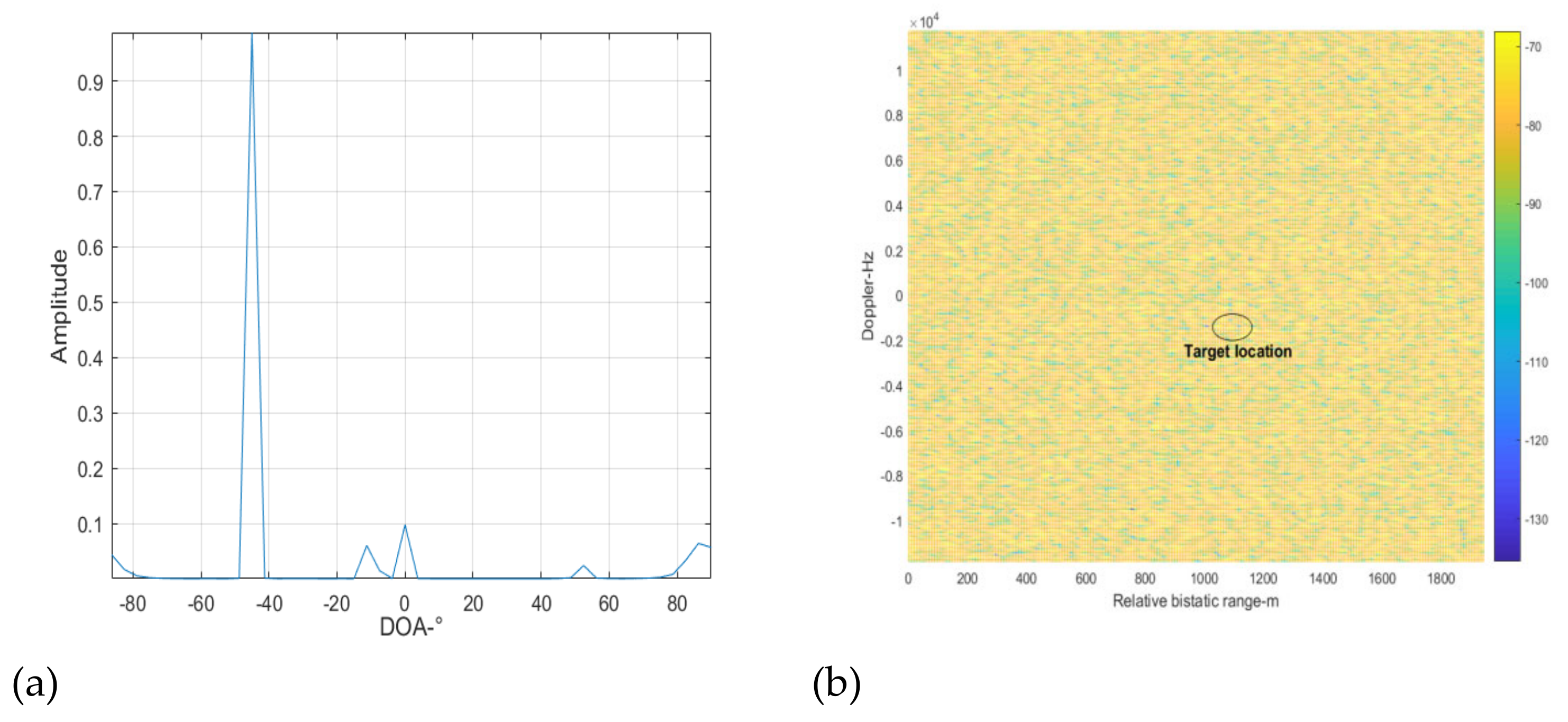
4. Simulation Analysis
5. Conclusions
Author Contributions
Funding
Institutional Review Board Statement
Informed Consent Statement
Data Availability Statement
Conflicts of Interest
References
- Willis, N.J.; Griffiths, H.D. (Eds.) Advances in Bistatic Radar; SciTech Publishing: Raleigh, NC, USA, 2007; Volume 2. [Google Scholar]
- Asif, A.; Kandeepan, S. Cooperative Fusion Based Passive Multistatic Radar Detection. Sensors 2021, 21, 3209. [Google Scholar] [CrossRef] [PubMed]
- Howland, P.E.; Maksimimuk, D.; Reitsma, G. FM radio based bistatic radar. IEE Proc. Radar Sonar Navig. 2005, 152, 107–115. [Google Scholar] [CrossRef] [Green Version]
- Edrich, M.; Schroeder, A.; Meyer, F. Design and performance evaluation of a mature FM/DAB/DVB-T multi-illuminator passive radar system. IET Radar Sonar Navig. 2014, 8, 114–122. [Google Scholar] [CrossRef]
- Searle, S.; Howard, S.; Palmer, J. Remodulation of DVB—T signals for use in Passive Bistatic Radar. In Proceedings of the 2010 Conference Record of the Forty Fourth Asilomar Conference on Signals, Systems and Computers, Pacific Grove, CA, USA, 7–10 November 2010; pp. 1112–1116. [Google Scholar] [CrossRef]
- Klincewicz, K.; Samczyński, P. Method of Calculating Desynchronization of DVB-T Transmitters Working in SFN for PCL Applications. Sensors 2020, 20, 5776. [Google Scholar] [CrossRef] [PubMed]
- He, Z.; Yang, Y.; Chen, W. A Hybrid Integration Method for Moving Target Detection with GNSS-Based Passive Radar. IEEE J. Sel. Top. Appl. Earth Obs. Remote Sens. 2021, 14, 1184–1193. [Google Scholar] [CrossRef]
- Abdullah, R.S.; Salah, A.A.; Ismail, A.; Hashim, F.H.; Rashid, N.E.A.; Abdul Aziz, N.H. Experimental investigation on target detection and tracking in passive radar using long-term evolution signal. IET Radar Sonar Navig. 2016, 10, 577–585. [Google Scholar] [CrossRef]
- Evers, A.; Jackson, J.A. Cross-ambiguity characterization of communication waveform features for passive radar. IEEE Trans. Aerosp. Electron. Syst. 2015, 51, 3440–3455. [Google Scholar] [CrossRef]
- Wang, H.T.; Lyu, X.Y.; Zhong, L.P. Interference to noise ratio estimation in LTE passive radar based on cyclic auto-correlation. Electron. Lett. 2021, 57, 375–377. [Google Scholar] [CrossRef]
- Garry, J.L.; Baker, C.J.; Smith, G.E. Evaluation of Direct Signal Suppression for Passive Radar. IEEE Trans Geosci. Remote Sens. 2017, 55, 3786–3799. [Google Scholar] [CrossRef]
- Shan, T.; Ma, Y.H.; Tao, R.; Liu, S. Multi-channel NLMS-based sea clutter cancellation in passive bistatic radar. IECE Electron. Express 2014, 11, 1–12. [Google Scholar]
- Colone, F.; O’hagan, D.W.; Lombardo, P.; Baker, C.J. A multistage processing algorithm for disturbance removal and target detection in passive bistatic radar. IEEE Trans. Aerosp. Electron. Syst. 2009, 45, 698–722. [Google Scholar] [CrossRef]
- Yi, J.; Wan, X.; Li, D.; Leung, H. Robust Clutter Rejection in Passive Radar via Generalized Subband Cancellation. IEEE Trans. Aerosp. Electron. Syst. 2018, 54, 1931–1946. [Google Scholar] [CrossRef]
- Stukovska, P.; Plsek, R. Clutter and distortion products suppression methods for code division multiple access systems. IET Radar Sonar Navig. 2019, 13, 1755–1763. [Google Scholar] [CrossRef]
- Griffiths, H.D.; Baker, C.J. The signal and interference environment in passive bistatic radar. In Proceedings of the Information, Decision and Control, Adelaide, SA, Australia, 12–14 February 2007; pp. 1–10. [Google Scholar]
- Lv, X.; Zhang, H.; Liu, Z.; Sun, Z.; Liu, P. Research on Co-channel Base Station Interference Suppression Method of Passive Radar Based on LTE Signal. J. Electron. Inf. Technol. 2019, 41, 2123–2130. (In Chinese) [Google Scholar]
- Barott, W.C.; Himed, B. Cochannel interference in ATSC passive radar. In Proceedings of the IEEE Radar Conference, Arlington, VA, USA, 10–15 May 2015; pp. 1270–1275. [Google Scholar]
- Lü, M.; Yi, J.; Wan, X.; Zhan, W. Cochannel Interference in DTMB-Based Passive Radar. IEEE Trans. Aerosp. Electron. Syst. 2019, 55, 2138–2149. [Google Scholar] [CrossRef]
- Hasan, B.; Mostafa, D.; Abbas, S. Dynamic Clutter Suppression and Multitarget Detection in a DVB-T Based Passive Radar. IEEE Trans. Aerosp. Electron. Syst. 2017, 53, 1812–1825. [Google Scholar]
- Zemmari, R.; Knoedler, B.; Nickel, U. GSM passive coherent location: Improving range resolution by mismatched filtering. In Proceedings of the 2013 IEEE Radar Conference (RadarCon13), Ottawa, ON, Canada, 29 April–3 May 2013; pp. 1–6. [Google Scholar] [CrossRef]
- Aldowesh, A.; Shoaib, M.; Jamil, K.; Alhumaidi, S.; Alam, M. A passive bistatic radar experiment for very low radar cross-section target detection. In Proceedings of the 2015 IEEE Radar Conference, Arlington, VA, USA, 27–30 October 2015; pp. 406–410. [Google Scholar] [CrossRef]
- Fabrizio, G.; Colone, F.; Lombardo, P.; Farina, A. Adaptive beamforming for high frequency over-the-horizon passive radar. IET Proceeding Radar Sonar Navig. 2009, 3, 384–405. [Google Scholar] [CrossRef]
- Wang Haitao, Wang Jun, Li Hongwei Target detection using CDMA based passive bistatic radar. J. Syst. Eng. Electron. 2012, 23, 858–865. [CrossRef]
- Vorobyov, S.A.; Gershman, A.B.; Luo, Z. Robust adaptive beamforming using worst-case performance optimization: A solution to the Signal Mismatch Problem. IEEE Trans. Signal Processing 2003, 51, 313–324. [Google Scholar] [CrossRef] [Green Version]
- 3GPP TS 36.211 V13.2.0. Physical Channels and Modulation. 3GPP Organizational Partners. July 2016.
- Kim, S.-J.; Koh, K.; Lustig, M.; Boyd, S.; Gorinevsky, D. An interior-point method for large-scale l1-regularized LSs. IEEE J. Sel. Top. Signal Process 2007, 1, 606–617. [Google Scholar] [CrossRef]


Publisher’s Note: MDPI stays neutral with regard to jurisdictional claims in published maps and institutional affiliations. |
© 2021 by the authors. Licensee MDPI, Basel, Switzerland. This article is an open access article distributed under the terms and conditions of the Creative Commons Attribution (CC BY) license (https://creativecommons.org/licenses/by/4.0/).
Share and Cite
Wang, H.; Lyu, X.; Liao, K. Co-Channel Interference Suppression for LTE Passive Radar Based on Spatial Feature Cognition. Sensors 2022, 22, 117. https://doi.org/10.3390/s22010117
Wang H, Lyu X, Liao K. Co-Channel Interference Suppression for LTE Passive Radar Based on Spatial Feature Cognition. Sensors. 2022; 22(1):117. https://doi.org/10.3390/s22010117
Chicago/Turabian StyleWang, Haitao, Xiaoyong Lyu, and Kefei Liao. 2022. "Co-Channel Interference Suppression for LTE Passive Radar Based on Spatial Feature Cognition" Sensors 22, no. 1: 117. https://doi.org/10.3390/s22010117
APA StyleWang, H., Lyu, X., & Liao, K. (2022). Co-Channel Interference Suppression for LTE Passive Radar Based on Spatial Feature Cognition. Sensors, 22(1), 117. https://doi.org/10.3390/s22010117