
Multi-Level Context Pyramid Network for Visual Sentiment Analysis

Abstract
1. Introduction
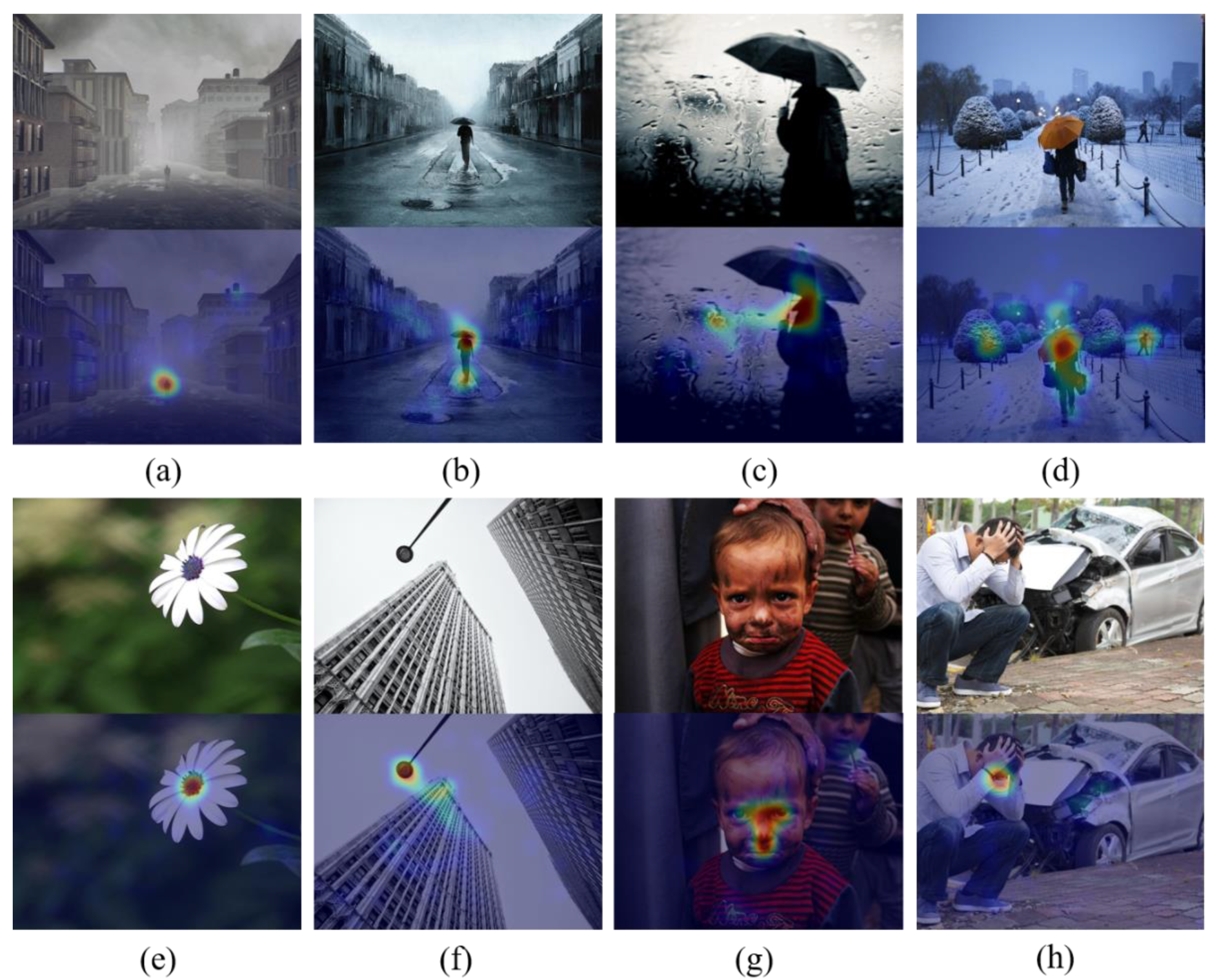
- Perception of different scale objects. The size and location of objects in images from social networks are diverse, which means that we need to have multi-scale analysis capabilities in the model. As shown in Figure 1, the scale of people in the images (a) to (c) is from small to large. Thus, a single-scale method object perception can only capture objects at a limited scale, while losing object information at other scales.
- Different levels of emotional representation. Different objects can evoke dissimilar degrees of sentiment. As shown in Figure 1e–h. Some simple objects contain less semantic information, such as the flower (e), and the street lamp (f). The emotional stimulation they express is weak, and their emotional information can be described by the low-level features. However, the complex semantic information will give us stronger emotional stimulation such as humans and human-related objects. Human’s non-verbal communication such as facial expression (g), body language and posture (h), have a strong ability to express emotions [13]. These complex objects need more abstract high-level semantic features to describe their emotional information.
- Adaptive context framework is introduced for the first time in the image sentiment analysis task. This method can learn the correlation degree of different regions in the image by combining different scale representations, which is helpful to improve the ability of the model to understand complex scenarios.
- The multi-scale attributes in the proposed MACM module are alterable. Compared with many existing multi-scale methods that can only capture objects of fixed limited scales, our method can combine different scales to capture objects of different positions and sizes in the image.
- The proposed MPCNet adopts cross-layer and multi-layer feature fusion strategies to enhance the ability of the model to perceive semantic objects at different levels.
- The experiment proves the advancement of our method, and the visualization results show that our method can effectively identify the small semantic objects related to emotional expression in complex scenarios.
2. Related Work
2.1. CNN with Additional Information
2.2. Region-Based CNN
2.3. Context-Based CNN
3. Methodology
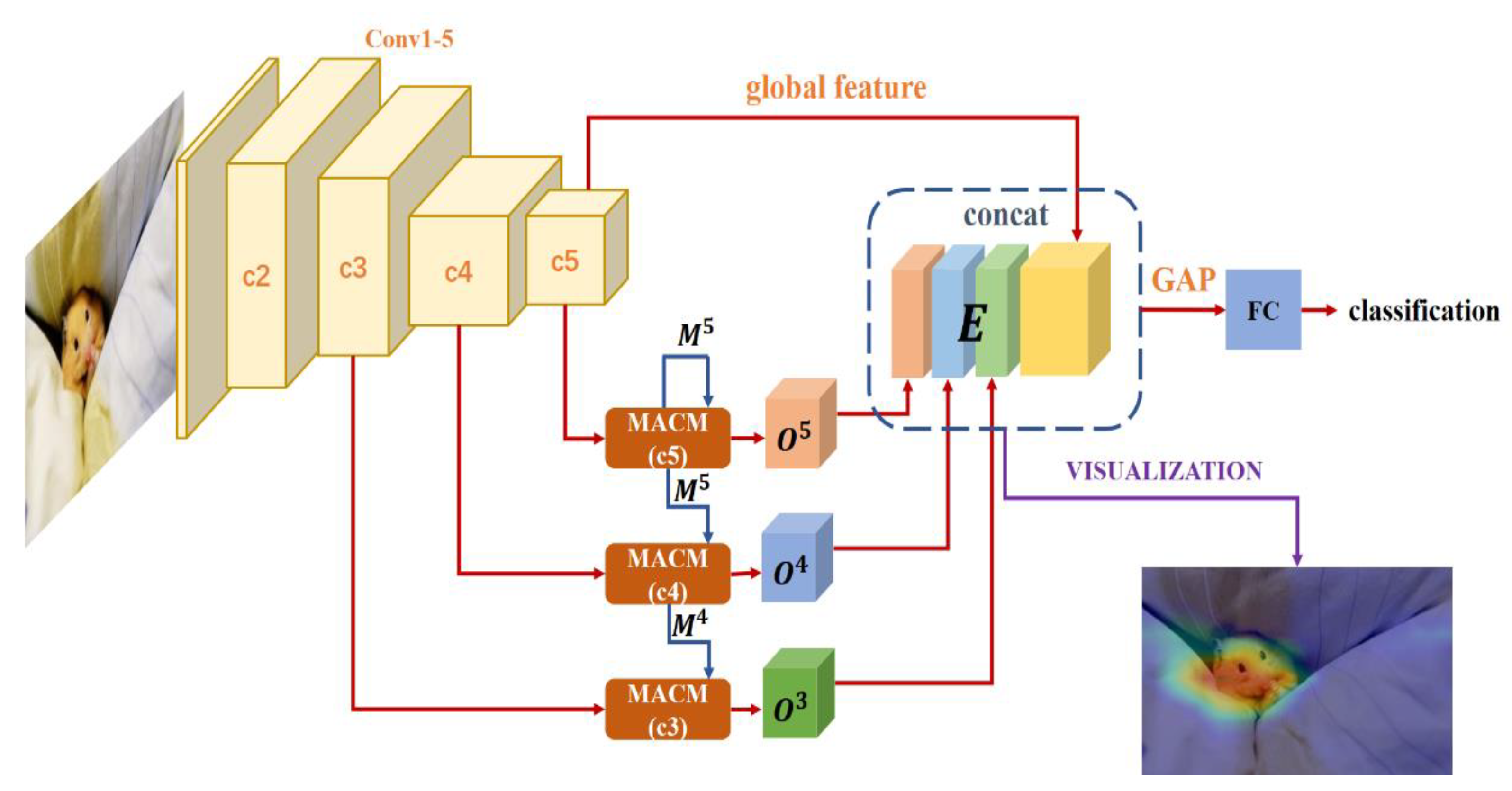
3.1. Proposed Multi-Level Context Pyramid Network
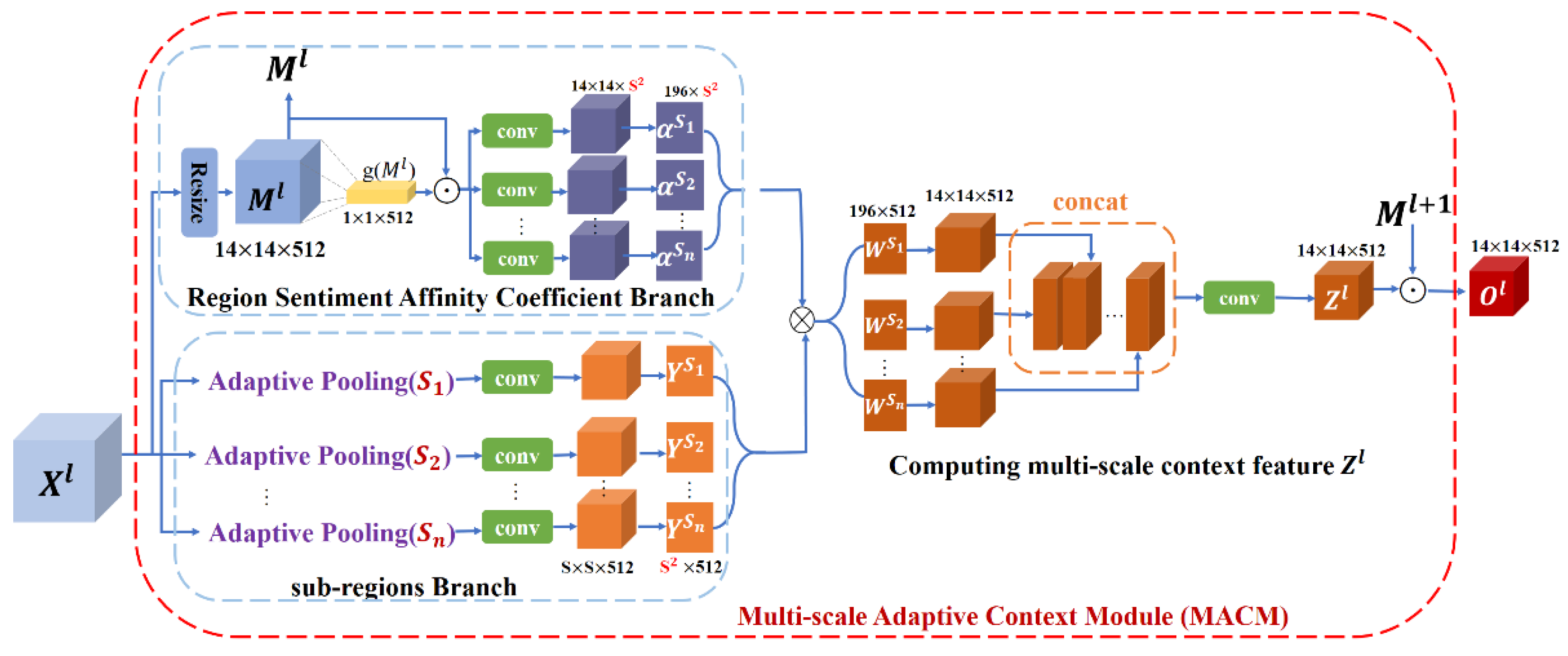
3.2. Multi-Scale Adaptive Context Module
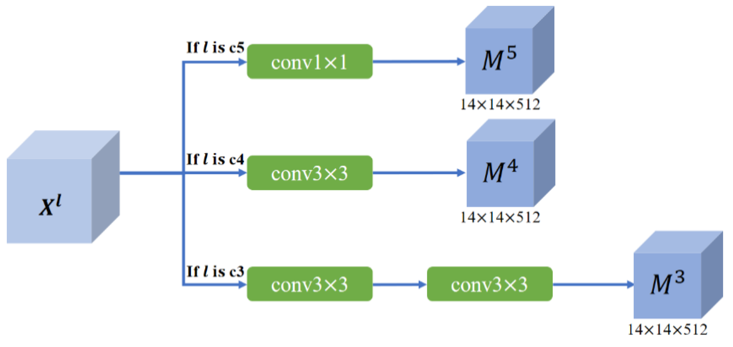
3.3. Cross-Layer and Multi-Layer Feature Fusion Strategies
4. Experiment
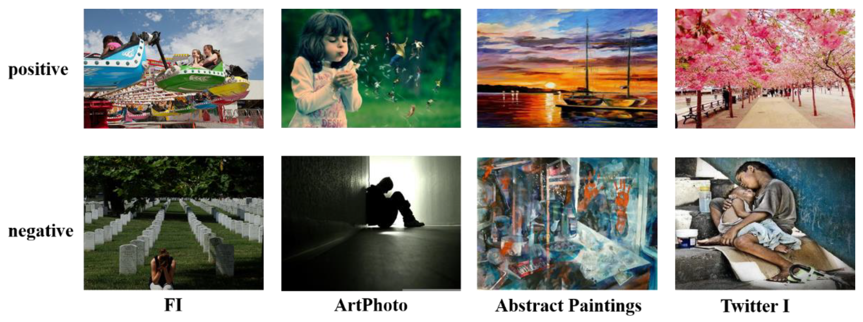
4.1. Dataset
- Small-scale dataset: IAPSsubset comes from International Affective Picture System [33] and has 395 images in eight emotional categories. Different from other datasets, ArtPhoto is a dataset composed of 806 art photos, and Abstract Paintings consists of 228 abstract pictures of colors and textures. Twitter I and Twitter II were collected from social network Twitter and labeled by AMT workers with 1,269 and 603 images. We set up experiments similar to [28,32] on all three subsets of Twitter I. EmotionROI is developed from Emotion6 [34], and the image comes from the Flickr website. Compared to Emotion6, EmotionROI adds 15 emotion-related annotation boxes to each image marked by participants and believes that the more repeated annotation boxes on a pixel point, the greater the contribution of the point to emotional expression.
- Large-scale dataset: FI is currently the most commonly used large-scale visual sentiment dataset, which is collected through social network using emotional categories as search keywords. 225 participants from AMT were employed to label resulting in 23,308 images.
4.2. Implementation Details
4.3. Baseline
4.3.1. Hand-Crafted Features
4.3.2. Features Based on CNN
4.4. Experimental Validation
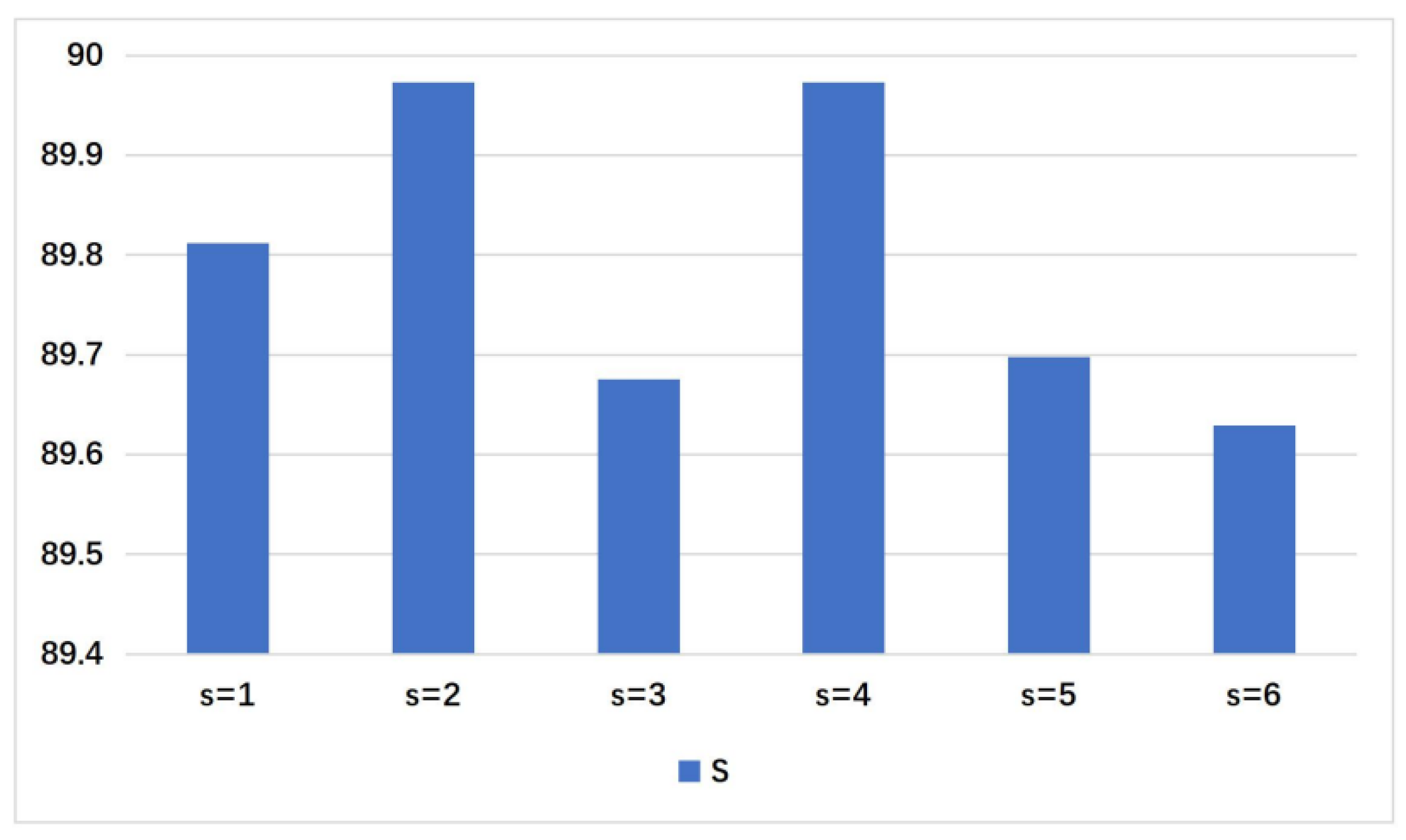
4.4.1. Choice of Scale
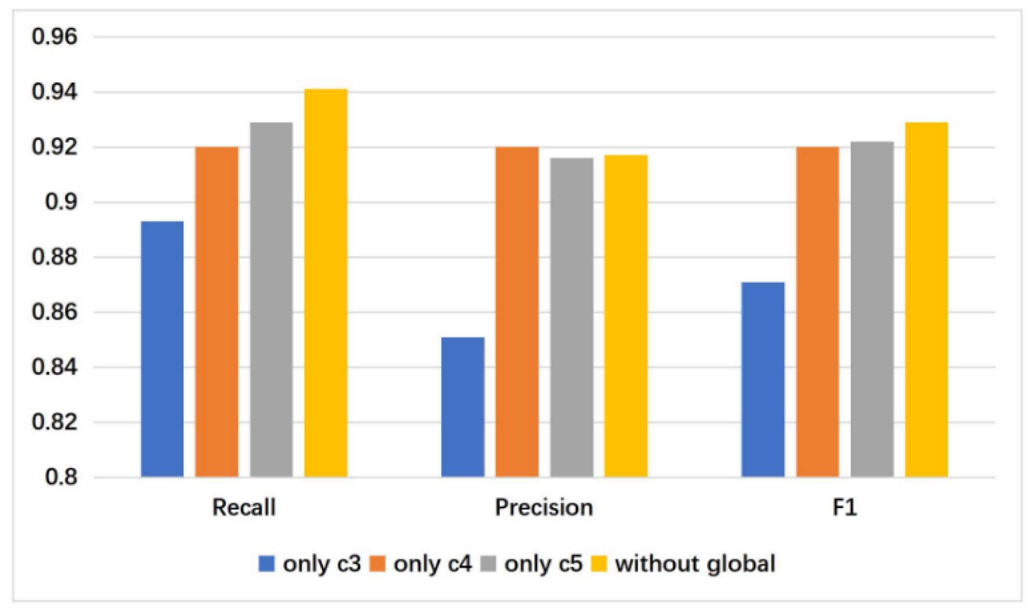
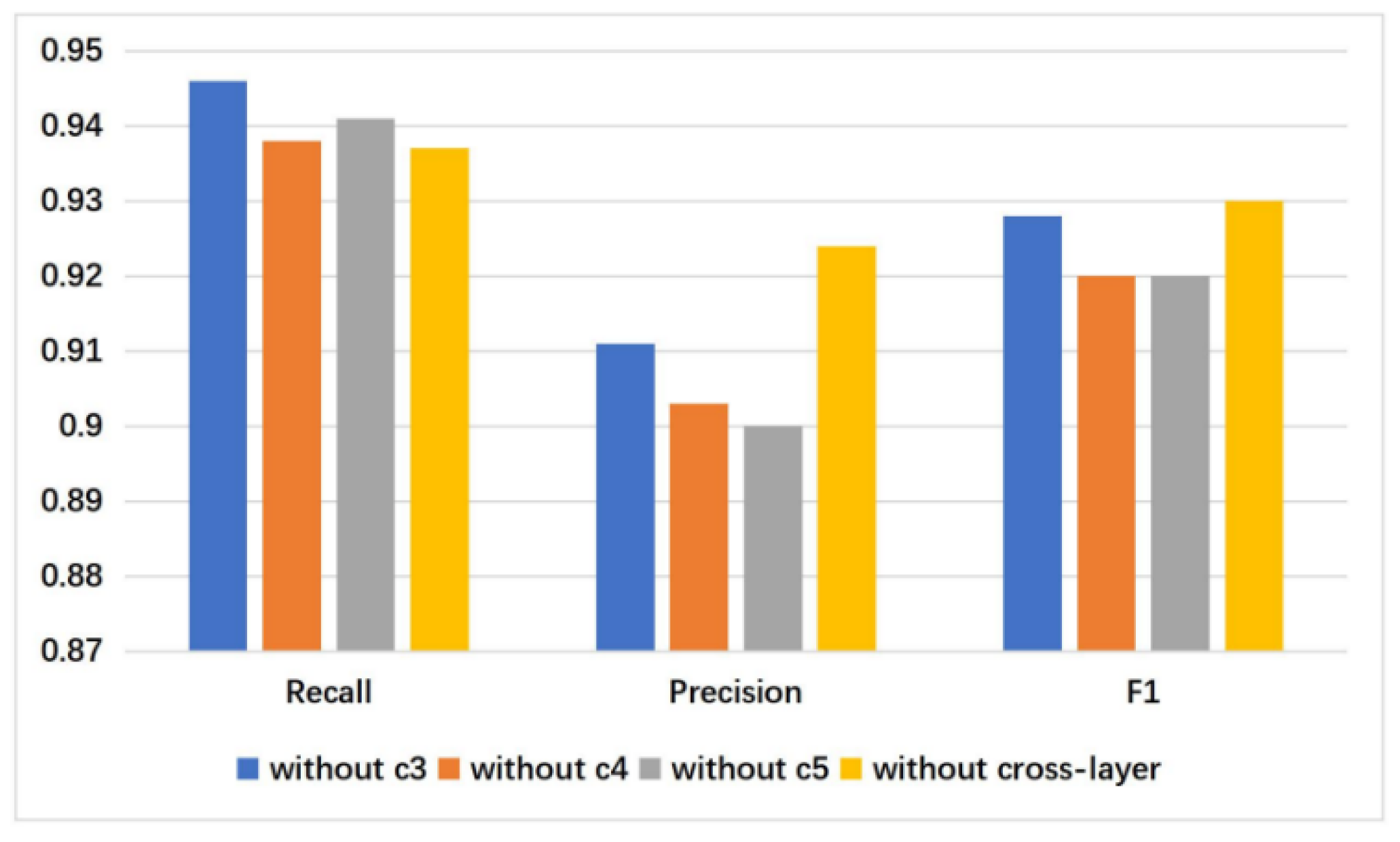
4.4.2. Effective of Different Level Features
4.5. Comparisons with State-of-the-Art Methods
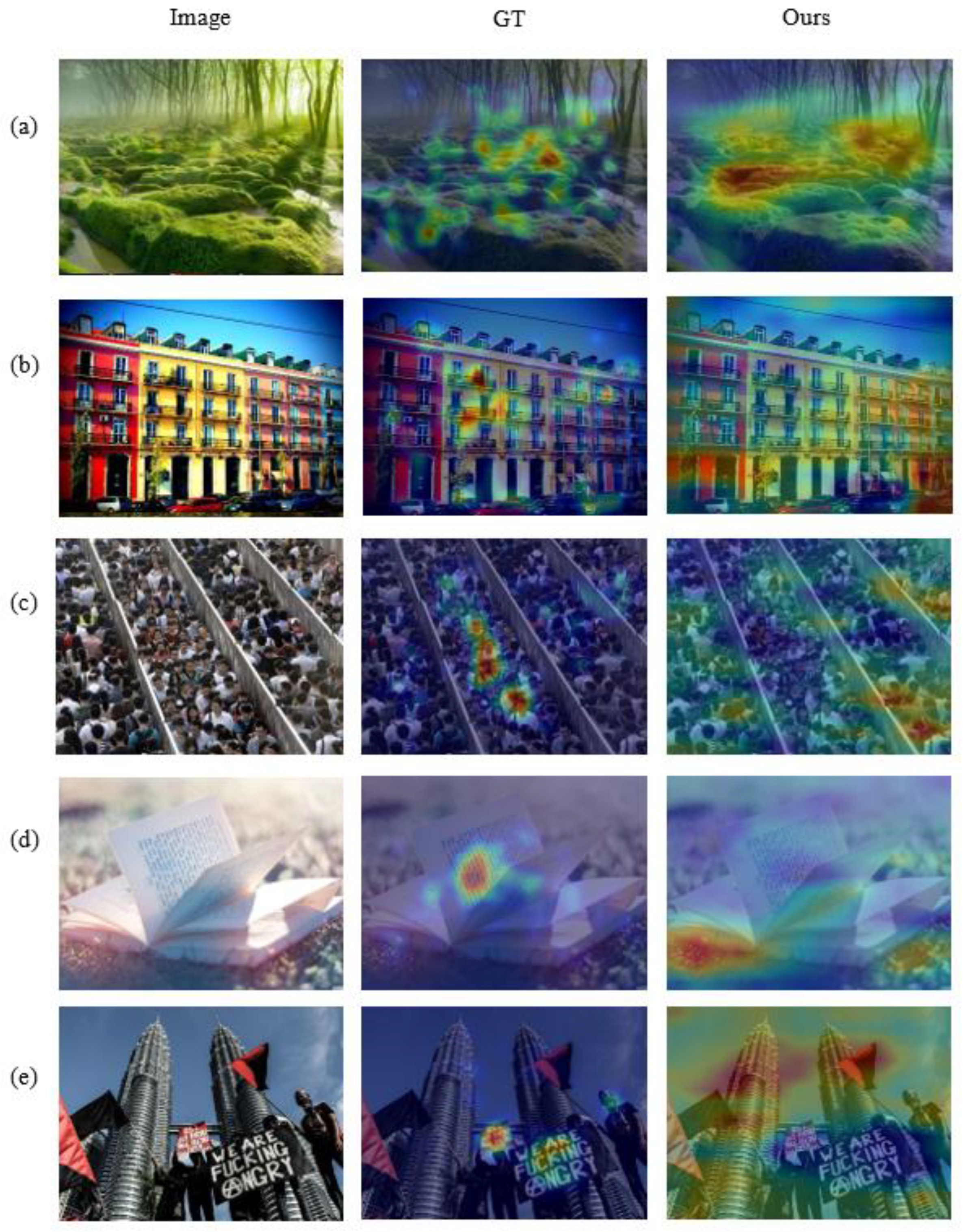
4.6. Visualization
5. Conclusions
Author Contributions
Funding
Institutional Review Board Statement
Informed Consent Statement
Data Availability Statement
Conflicts of Interest
References
- Fan, S.; Shen, Z.; Jiang, M.; Koenig, B.L.; Xu, J.; Kankanhalli, M.S.; Zhao, Q. Emotional attention: A study of image sentiment and visual attention. In Proceedings of the IEEE Conference on Computer Vision and Pattern Recognition, Salt Lake City, UT, USA, 18–22 June 2018. [Google Scholar]
- Brosch, T.; Pourtois, G.; Sander, D. The perception and categorisation of emotional stimuli: A review. Cogn. Emot. 2010, 24, 377–400. [Google Scholar] [CrossRef]
- Ortis, A.; Farinella, G.M.; Battiato, S. Survey on visual sentiment analysis. IET Image Process. 2020, 14, 1440–1456. [Google Scholar] [CrossRef]
- Rao, T.; Li, X.; Zhang, H.; Xu, M. Multi-level region-based convolutional neural network for image emotion classification. Neurocomputing 2019, 333, 429–439. [Google Scholar] [CrossRef]
- Joshi, D.; Datta, R.; Fedorovskaya, E.; Luong, Q.T.; Wang, J.Z.; Li, J.; Luo, J. Aesthetics and emotions in images. IEEE Signal Process. Mag. 2011, 28, 94–115. [Google Scholar] [CrossRef]
- You, Q.; Jin, H.; Luo, J. Visual sentiment analysis by attending on local image regions. In Proceedings of the Thirty-First AAAI Conference on Artificial Intelligence, San Francisco, CA, USA, 4–9 February 2017; Volume 31. [Google Scholar]
- Fan, S.; Jiang, M.; Shen, Z.; Koenig, B.L.; Kankanhalli, M.S.; Zhao, Q. The role of visual attention in sentiment prediction. In Proceedings of the 25th ACM International Conference on Multimedia, Mountain View, CA, USA, 23–27 October 2017; pp. 217–225. [Google Scholar]
- Song, K.; Yao, T.; Ling, Q.; Mei, T. Boosting image sentiment analysis with visual attention. Neurocomputing 2018, 312, 218–228. [Google Scholar] [CrossRef]
- Rao, T.; Li, X.; Xu, M. Learning multi-level deep representations for image emotion classification. Neural Process. Lett. 2019, 1–19. [Google Scholar] [CrossRef]
- Chen, T.; Yu, F.X.; Chen, J.; Cui, Y.; Chen, Y.Y.; Chang, S.F. Object-based visual sentiment concept analysis and application. In Proceedings of the 22nd ACM international conference on Multimedia, Orlando, FL, USA, 3–7 November 2014. [Google Scholar]
- Zhao, Q.; Sheng, T.; Wang, Y.; Tang, Z.; Chen, Y.; Cai, L.; Ling, H. M2det: A single-shot object detector based on multi-level feature pyramid network. In Proceedings of the AAAI Conference on Artificial Intelligence, Honolulu, HI, USA, 27 January–1 February 2019; Volume 33, pp. 9259–9266. [Google Scholar]
- He, J.; Deng, Z.; Zhou, L.; Wang, Y.; Qiao, Y. Adaptive pyramid context network for semantic segmentation. In Proceedings of the IEEE Conference on Computer Vision and Pattern Recognition, Long Beach, CA, USA, 16–20 June 2019. [Google Scholar]
- Surekha, S. Deep Neural Network-based human emotion recognition by computer vision, Advances in Electrical and Computer Technologies. Springer LNEE 2020, 672, 453–463. [Google Scholar]
- Cerf, M.; Frady, E.P.; Koch, C. Faces and text attract gaze independent of the task: Experimental data and computer model. J. Vis. 2009, 9, 10–11. [Google Scholar] [CrossRef] [PubMed]
- You, Q.; Luo, J.; Jin, H.; Yang, J. Building a large scale dataset for image emotion recognition: The fine print and the benchmark. In Proceedings of the Thirtieth AAAI Conference on Artificial Intelligence, Phoenix, AZ, USA, 12–17 February 2016. [Google Scholar]
- Borth, J.R.; Chen, T.; Breuel, T.; Chang, S.F. Large-scale visual sentiment ontology and detectors using adjective noun pairs. In Proceedings of the 21st ACM International Conference on Multimedia, Barcelona, Spain, 21–25 October 2013. [Google Scholar]
- Chen, T.; Borth, D.; Darrell, T.; Chang, S.F. DeepSentiBank: Visual Sentiment Concept Classification with Deep Convolutional Neural Networks. arXiv 2014, arXiv:1410.8586. [Google Scholar]
- Li, Z.; Fan, Y.; Liu, W.; Wang, F. Image sentiment prediction based on textual descriptions with adjective noun pairs. Multimed. Tools Appl. 2018, 77, 1115–1132. [Google Scholar] [CrossRef]
- Yuan, J.; Mcdonough, S.; You, Q.; Luo, J. Sentribute: Image sentiment analysis from a mid-level perspective. In Proceedings of the Second International Workshop on Issues of Sentiment Discovery and Opinion Mining, Chicago, IL, USA, 11–14 August 2013. [Google Scholar]
- Yang, J.; She, D.; Ming, S. Joint Image Emotion Classification and Distribution Learning via Deep Convolutional Neural Network. In Proceedings of the Twenty-sixth International Joint Conference on Artificial Intelligence, Melbourne, Australia, 19–25 August 2017. [Google Scholar]
- Kim, H.R.; Kim, S.J.; Lee, I.K. Building emotional machines: Recognizing image emotions through deep neural networks. IEEE Trans. Multimed. 2018, 20, 2980–2992. [Google Scholar] [CrossRef]
- Ali, A.R.; Shahid, U.; Ali, M.; Ho, J. High-level concepts for affective understanding of images. In Proceedings of the 2017 IEEE Winter Conference on Applications of Computer Vision (WACV), Santa Rosa, CA, USA, 27–29 March 2017. [Google Scholar]
- Peng, K.C.; Sadovnik, A.; Gallagher, A.; Chen, T. Where do emotions come from? predicting the emotion stimuli map. In Proceedings of the 2016 IEEE International Conference on Image Processing (ICIP), Phoenix, AZ, USA, 25–28 September 2016. [Google Scholar]
- Zhou, B.; Khosla, A.; Lapedriza, A.; Oliva, A.; Torralba, A. Object detectors emerge in deep scene cnns. International Conference on Learning Representations; San Diego, CA, USA, 7–9 May 2015. [Google Scholar]
- Yang, J.; She, D.; Lai, Y.K.; Rosin, P.L.; Yang, M.H. Weakly supervised coupled networks for visual sentiment analysis. In Proceedings of the IEEE Conference on Computer Vision and Pattern Recognition, Salt Lake City, UT, USA, 18–22 June 2018. [Google Scholar]
- Yadav, A.; Vishwakarma, D.K. A deep learning architecture of RA-DLNet for visual sentiment analysis. Multimed. Syst. 2020, 26, 431–451. [Google Scholar] [CrossRef]
- Wu, L.; Qi, M.; Jian, M.; Zhang, H. Visual Sentiment Analysis by Combining Global and Local Information. Neural Process. Lett. 2020, 51, 2063–2075. [Google Scholar] [CrossRef]
- Yang, J.; She, D.; Sun, M.; Cheng, M.M.; Rosin, P.L.; Wang, L. Visual sentiment prediction based on automatic discovery of affective regions. IEEE Trans. Multimed. 2018, 20, 2513–2525. [Google Scholar] [CrossRef]
- Ren, S.; He, K.; Girshick, R.; Sun, J. Faster r-cnn: Towards real-time object detection with region proposal networks. IEEE Trans. Pattern Anal. Mach. Intell. 2017, 39, 1137–1149. [Google Scholar] [CrossRef]
- Mikels, J.A.; Fredrickson, B.L.; Larkin, G.R.; Lindberg, C.M.; Maglio, S.J.; Reuter-Lorenz, P.A. Emotional category data on images from the International Affective Picture System. Behav. Res. Methods 2005, 37, 626–630. [Google Scholar] [CrossRef] [PubMed]
- Machajdik, J.; Hanbury, A. Affective image classification using features inspired by psychology and art theory. In Proceedings of the 18th ACM International Conference on Multimedia, Firenze, Italy, 25–29 October 2010. [Google Scholar]
- You, Q.; Luo, J.; Jin, H.; Yang, J. Robust image sentiment analysis using progressively trained and domain transferred deep networks. In Proceedings of the Twenty-Ninth AAAI Conference on Artificial Intelligence, Austin, TX, USA, 25–30 January 2015. [Google Scholar]
- Lang, P.J.; Bradley, M.M.; Cuthbert, B.N. International affective picture system (IAPS): Technical manual and affective ratings. NIMH Cent. Study Emot. Atten. 1997, 1, 39–58. [Google Scholar]
- Peng, K.C.; Chen, T.; Sadovnik, A.; Gallagher, A. A mixed bag of emotions: Model, predict, and transfer emotion distributions. In Proceedings of the Computer Vision & Pattern Recognition IEEE, Boston, MA, USA, 8–12 June 2015. [Google Scholar]
- Panda, R.; Zhang, J.; Li, H.; Lee, J.Y.; Lu, X.; Roy-Chowdhury, A.K. Contemplating visual emotions: Understanding and overcoming dataset bias. In Proceedings of the European Conference on Computer Vision (ECCV), Munich, Germany, 8–14 September 2018. [Google Scholar]
- Ekman, P.; Friesen, W.V.; Ellsworth, P. What emotion categories or dimensions can observers judge from facial behavior? Emot. Hum. Face 1982, 39–55. [Google Scholar] [CrossRef]
- He, K.; Zhang, X.; Ren, S.; Sun, J. Deep residual learning for image recognition. In Proceedings of the IEEE Conference on Computer Vision and Pattern Recognition, Las Vegas, NV, USA, 27–30 June 2016. [Google Scholar]
- Siersdorfer, S.; Minack, E.; Deng, F.; Hare, J. Analyzing and predicting sentiment of images on the social web. In Proceedings of the 18th ACM international conference on Multimedia, Firenze, Italy, 25–29 October 2010. [Google Scholar]
- Zhao, S.; Gao, Y.; Jiang, X.; Yao, H.; Chua, T.S.; Sun, X. Exploring principles-of-art features for image emotion recognition. In Proceedings of the 22nd ACM International Conference on Multimedia, Orlando, FL, USA, 3–7 November 2014. [Google Scholar]
- Rao, T.; Xu, M.; Liu, H.; Wang, J.; Burnett, I. Multi-scale blocks based image emotion classification using multiple instance learning. In Proceedings of the 2016 IEEE International Conference on Image Processing (ICIP). IEEE, Phoenix, AZ, USA, 25–28 September 2016. [Google Scholar]
- Krizhevsky, A.; Sutskever, I.; Hinton, G.E. Imagenet classification with deep convolutional neural networks. Commun. ACM 2017, 60, 84–90. [Google Scholar] [CrossRef]
- Simonyan, K.; Zisserman, A. Very Deep Convolutional Networks for Large-Scale Image Recognition. arXiv 2014, arXiv:1409.1556. [Google Scholar]
- Zhu, X.; Li, L.; Zhang, W.; Rao, T.; Xu, M.; Huang, Q.; Xu, D. Dependency exploitation: A unified CNN-RNN approach for visual emotion recognition. In Proceedings of the 26th International Joint Conference on Artificial Intelligence, Melbourne, Australia, 19–25 August 2017. [Google Scholar]
- COCO: Common Objects in Context. 2016. Available online: http://mscoco.org/dataset/#detections-leaderboard (accessed on 25 July 2016).
- Zhou, B.; Khosla, A.; Lapedriza, A.; Oliva, A.; Torralba, A. Learning deep features for discriminative localization. In Proceedings of the IEEE Conference on Computer Vision and Pattern Recognition, Las Vegas, NV, USA, 27–30 June 2016. [Google Scholar]


| Dataset | Positive | Negative | Sum | Type |
|---|---|---|---|---|
| IAPSsubset [30] | 209 | 186 | 395 | natural |
| Abstract [31] | 139 | 89 | 228 | abstract |
| ArtPhoto [31] | 378 | 428 | 806 | artistic |
| Twitter I [32] | 769 | 500 | 1269 | social |
| Twitter II [16] | 463 | 133 | 596 | social |
| EmotionROI [23] | 660 | 1320 | 1980 | social |
| FI [15] | 16430 | 6878 | 23308 | social |
| Feature | Only | Without |
|---|---|---|
| 90.004 | - | |
| global | - | 89.789 |
| 89.011 | 88.393 | |
| 88.668 | 88.484 | |
| 81.250 | 89.675 | |
| ours | 90.31 | 90.31 |
| Method | FI | ArtPhoto | Abstract | IAPSsubset | EmotionROI |
|---|---|---|---|---|---|
| LCH [38] | 45.37 | 64.33 | 70.93 | 52.84 | 63.79 |
| GCH [38] | 47.95 | 66.53 | 67.33 | 69.96 | 66.85 |
| PAEF [39] | 58.42 | 68.42 | 66.23 | 65.77 | 73.45 |
| Rao(a) [40] | 62.79 | 71.53 | 67.82 | 78.34 | 74.51 |
| SentiBank [16] | 56.47 | 67.33 | 64.30 | 80.57 | 65.73 |
| AlexNet [41] | 68.63 | 69.27 | 65.49 | 84.58 | 71.60 |
| VGG-16 [42] | 73.95 | 70.48 | 65.88 | 87.20 | 72.49 |
| ResNet101 [37] | 75.76 | 71.08 | 66.64 | 88.15 | 73.92 |
| DeepSentiBank [17] | 64.39 | 70.26 | 69.07 | 86.31 | 70.38 |
| PCNN [32] | 73.59 | 71.47 | 70.26 | 88.65 | 74.06 |
| Rao(b) [9] | 79.54 | 74.83 | 71.96 | 90.53 | 78.99 |
| Zhu [43] | 84.26 | 75.50 | 73.88 | 91.38 | 80.52 |
| AR [28] | 86.35 | 74.80 | 76.03 | 92.39 | 81.26 |
| Rao(c) [4] | 87.51 | 78.36 | 77.28 | 93.66 | 82.94 |
| ours | 90.31 | 79.24 | 78.14 | 94.82 | 85.10 |
| Method | Twitter I | Twitter II | ||
|---|---|---|---|---|
| Twitter I_5 | Twitter I_4 | Twitter I_3 | ||
| GCH [38] | 67.91 | 67.20 | 65.41 | 77.68 |
| LCH [38] | 70.18 | 68.54 | 65.93 | 75.98 |
| PAEF [39] | 72.90 | 69.61 | 67.92 | 77.51 |
| SentiBank [16] | 71.32 | 68.28 | 66.63 | 65.93 |
| DeepSentiBank [17] | 76.35 | 70.15 | 71.25 | 70.23 |
| PCNN [32] | 82.54 | 76.52 | 76.36 | 77.68 |
| VGG-16 [42] | 83.44 | 78.67 | 75.49 | 71.79 |
| AR [28] | 88.65 | 85.10 | 81.06 | 80.48 |
| RA-DLNet [26] | 89.10 | 83.20 | 81.30 | 81.20 |
| GMEI &LRMSI [27] | 89.50 | 86.97 | 81.65 | 80.97 |
| ours | 89.77 | 86.57 | 83.88 | 81.19 |
Publisher’s Note: MDPI stays neutral with regard to jurisdictional claims in published maps and institutional affiliations. |
© 2021 by the authors. Licensee MDPI, Basel, Switzerland. This article is an open access article distributed under the terms and conditions of the Creative Commons Attribution (CC BY) license (http://creativecommons.org/licenses/by/4.0/).
Share and Cite
Ou, H.; Qing, C.; Xu, X.; Jin, J. Multi-Level Context Pyramid Network for Visual Sentiment Analysis. Sensors 2021, 21, 2136. https://doi.org/10.3390/s21062136
Ou H, Qing C, Xu X, Jin J. Multi-Level Context Pyramid Network for Visual Sentiment Analysis. Sensors. 2021; 21(6):2136. https://doi.org/10.3390/s21062136
Chicago/Turabian StyleOu, Haochun, Chunmei Qing, Xiangmin Xu, and Jianxiu Jin. 2021. "Multi-Level Context Pyramid Network for Visual Sentiment Analysis" Sensors 21, no. 6: 2136. https://doi.org/10.3390/s21062136
APA StyleOu, H., Qing, C., Xu, X., & Jin, J. (2021). Multi-Level Context Pyramid Network for Visual Sentiment Analysis. Sensors, 21(6), 2136. https://doi.org/10.3390/s21062136