Author Contributions
Conceptualization, Y.L. and C.L.; methodology, Y.L. and M.J.; software, Y.L. and G.C.; formal analysis, Y.L., M.J. and G.C.; data curation, M.J. and G.C.; writing—original draft preparation, Y.L., M.J. and C.L.; writing—review and editing, M.J. and C.J.; visualization, G.C. and C.J.; supervision, C.L.; project administration, C.L.; funding acquisition, C.L. All authors have read and agreed to the published version of the manuscript.
Figure 1.
Smart data characterization procedure from raw data.
Figure 1.
Smart data characterization procedure from raw data.
Figure 3.
Experimental data acquisition by sensor position designation within the printing section.
Figure 3.
Experimental data acquisition by sensor position designation within the printing section.
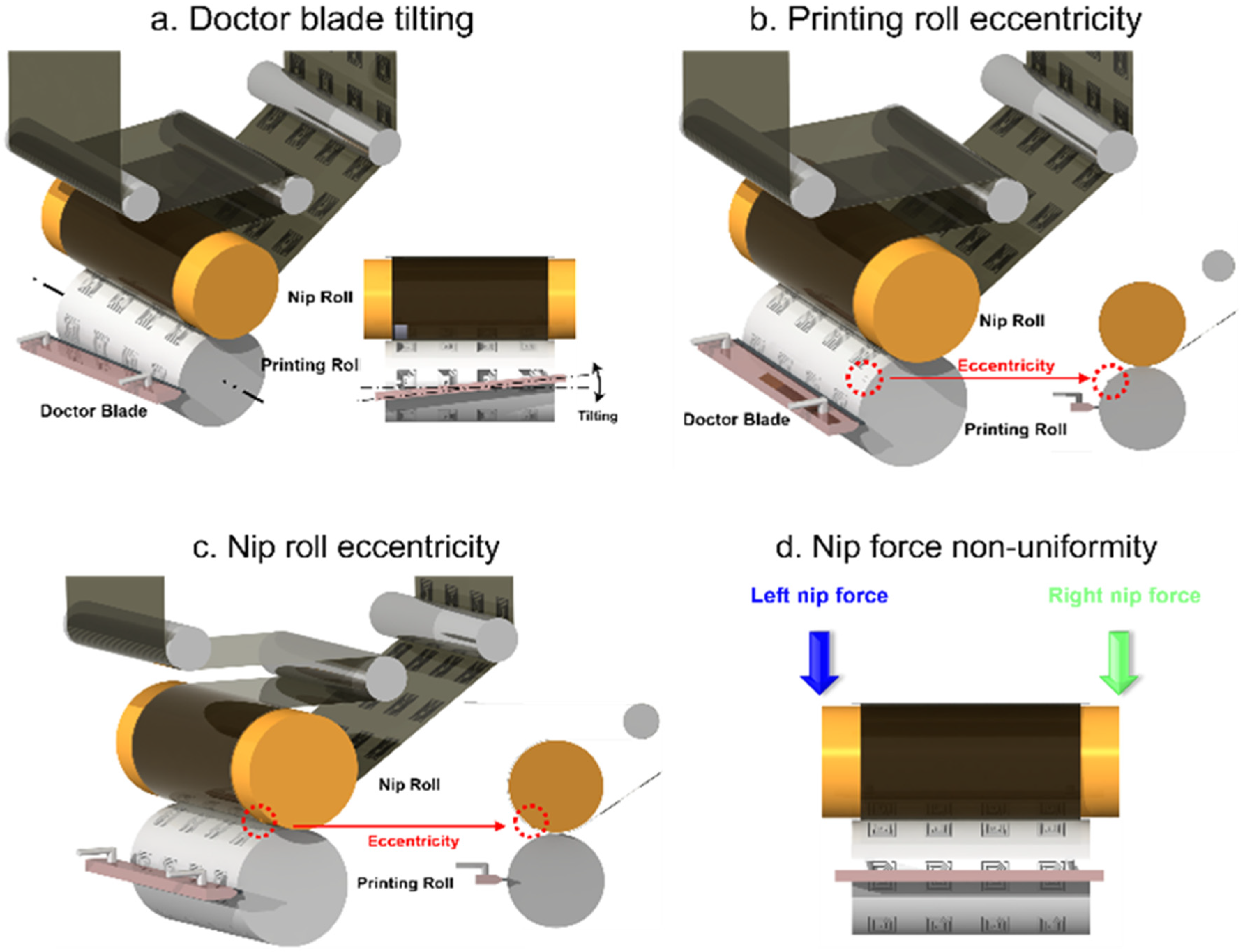
Figure 4.
Possible main faults during gravure printing process: (a) Doctor blade tilting fault; (b) Printing roll eccentricity fault; (c) Nip roll eccentricity fault; and (d) Nip force non-uniformity fault.
Figure 4.
Possible main faults during gravure printing process: (a) Doctor blade tilting fault; (b) Printing roll eccentricity fault; (c) Nip roll eccentricity fault; and (d) Nip force non-uniformity fault.
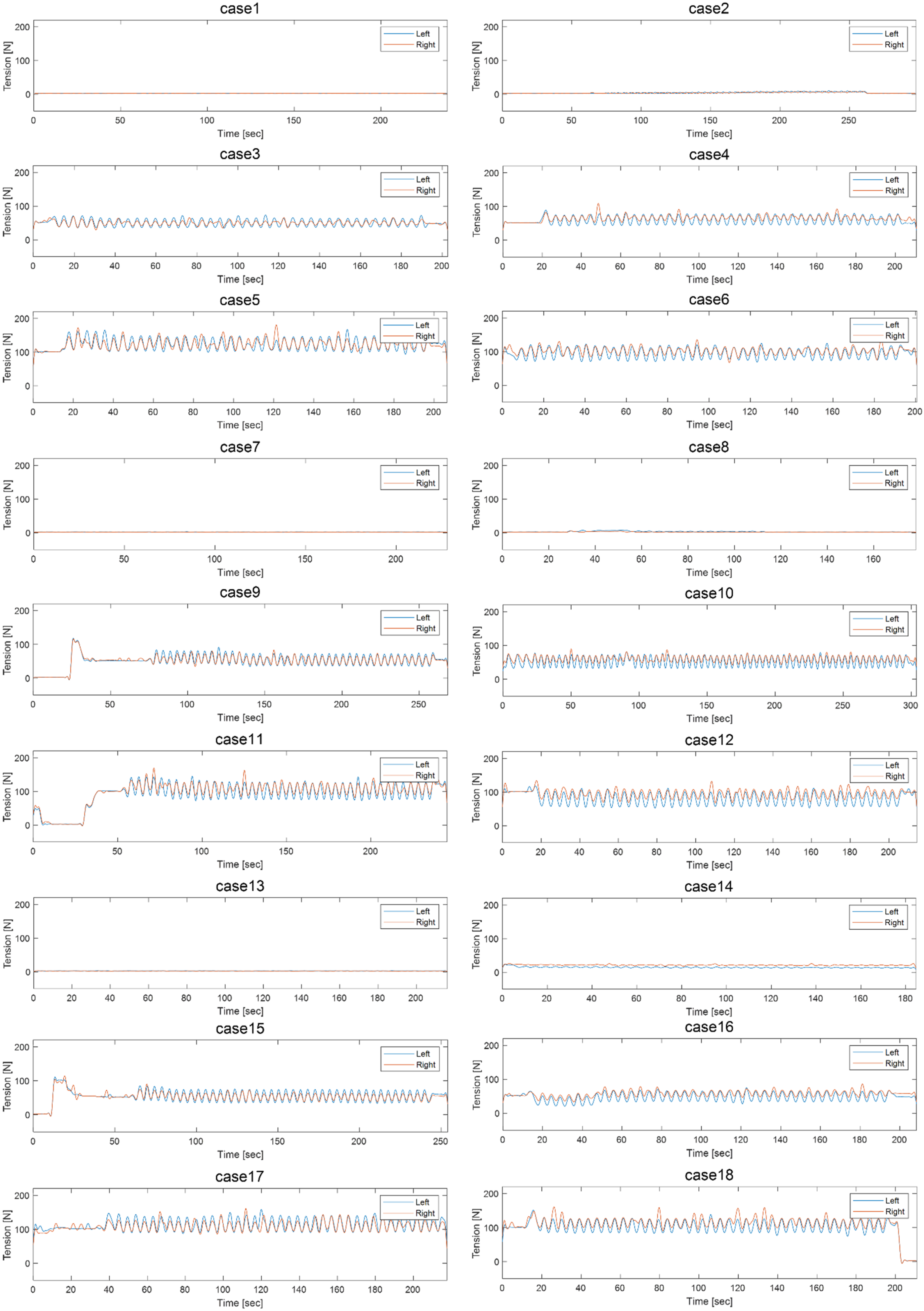
Figure 5.
Nip force uniformity data of Cases 1–18.
Figure 5.
Nip force uniformity data of Cases 1–18.
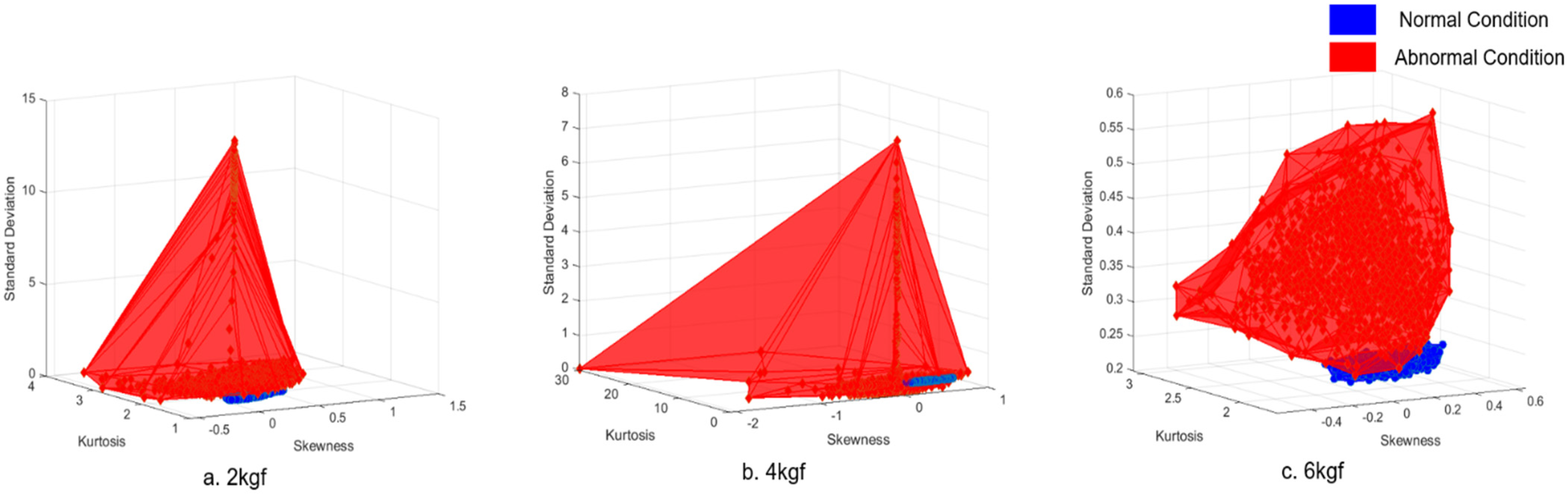
Figure 6.
Volume comparison of normal and abnormal condition data: (a) Operating tension of 2 kgf; (b) Operating tension of 4 kgf; and (c) Operating tension of 6 kgf.
Figure 6.
Volume comparison of normal and abnormal condition data: (a) Operating tension of 2 kgf; (b) Operating tension of 4 kgf; and (c) Operating tension of 6 kgf.
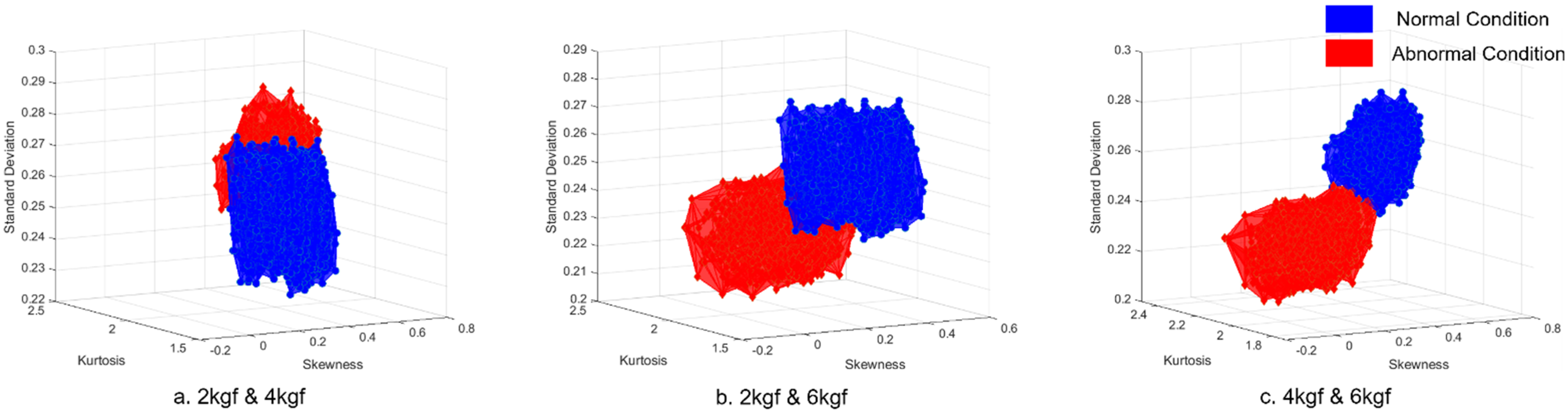
Figure 7.
Volume comparison of normal and abnormal condition data: (a) Operating tensions of 2 and 4 kgf; (b) Operating tensions of 2 and 6 kgf; and (c) Operating tensions of 4 and 6 kgf.
Figure 7.
Volume comparison of normal and abnormal condition data: (a) Operating tensions of 2 and 4 kgf; (b) Operating tensions of 2 and 6 kgf; and (c) Operating tensions of 4 and 6 kgf.
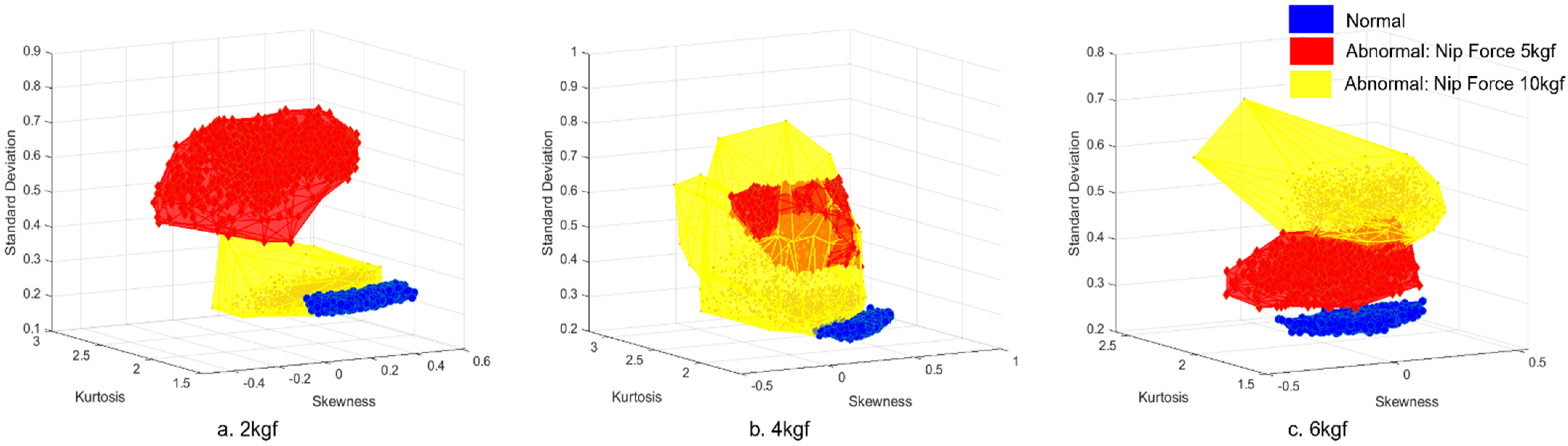
Figure 8.
Volume comparison of normal and abnormal condition data: (a) Operating tension of 2 kgf; (b) Operating tension of 4 kgf; and (c) Operating tension of 6 kgf.
Figure 8.
Volume comparison of normal and abnormal condition data: (a) Operating tension of 2 kgf; (b) Operating tension of 4 kgf; and (c) Operating tension of 6 kgf.
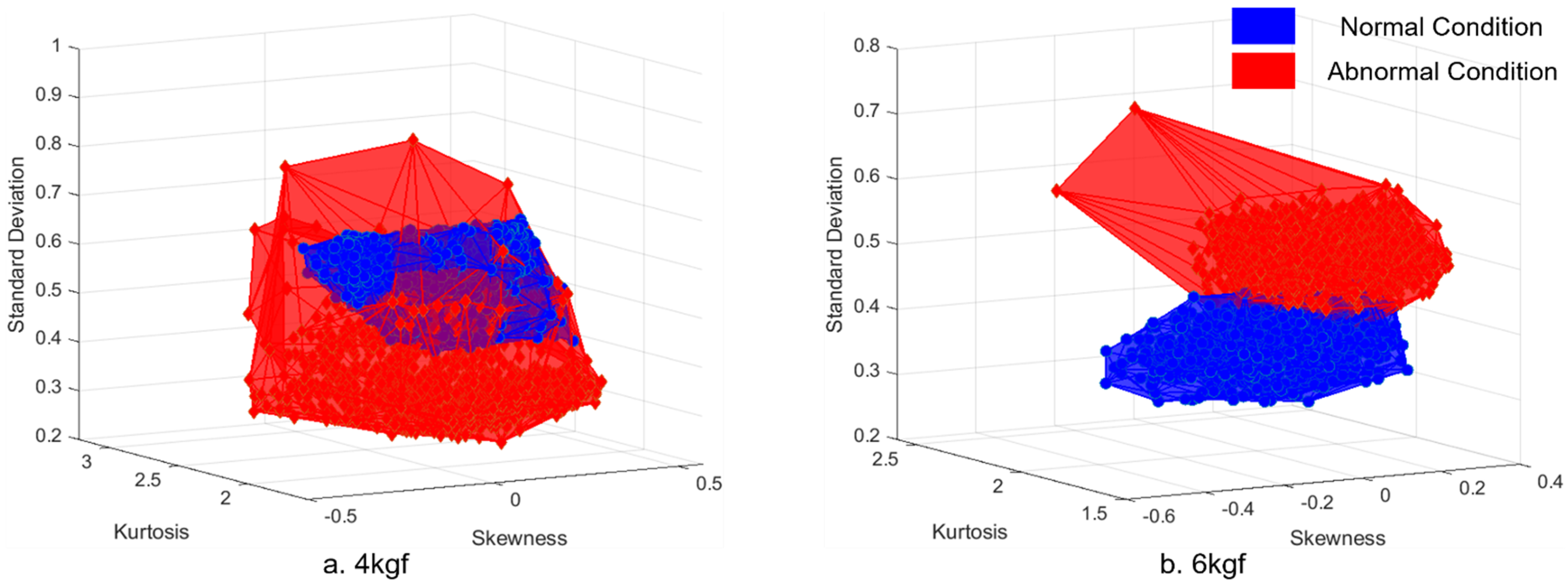
Figure 9.
Volume comparison of normal and abnormal condition data: (a) Operating tension of 4 kgf; (b) Operating tension of 6 kgf.
Figure 9.
Volume comparison of normal and abnormal condition data: (a) Operating tension of 4 kgf; (b) Operating tension of 6 kgf.
Table 1.
Specifications of acceleration sensor and NI-9230 module.
Table 1.
Specifications of acceleration sensor and NI-9230 module.
| Item | Parameter | Value |
|---|
| Sensor | Sensor Type | Share Accelerometer, Triaxial |
| Sensitivity ] | 5.15 |
| Measurement Range ] | 1000 g peak |
| Frequency Range [Hz] | 2–5000 Hz |
| Resolution ] | 0.003 (rms) |
| Module | Sampling Rate Range [Hz] | 0–1651.6 |
| Sampling Time per Trial [s] | 36,000 |
Table 2.
Experimental design of data acquisition with experimental variables of tension, nip force, and doctoring.
Table 2.
Experimental design of data acquisition with experimental variables of tension, nip force, and doctoring.
| Case No. | Tension [kgf] | Nip Force [kgf] | Doctoring |
|---|
| 1 | 2 | Without Nipping | Without Doctoring |
| 2 | Without Nipping | With Doctoring |
| 3 | 5 | Without Doctoring |
| 4 | 5 | With Doctoring |
| 5 | 10 | Without Doctoring |
| 6 | 10 | With Doctoring |
| 7 | 4 | Without Nipping | Without Doctoring |
| 8 | Without Nipping | With Doctoring |
| 9 | 5 | Without Doctoring |
| 10 | 5 | With Doctoring |
| 11 | 10 | Without Doctoring |
| 12 | 10 | With Doctoring |
| 13 | 6 | Without Nipping | Without Doctoring |
| 14 | Without Nipping | With Doctoring |
| 15 | 5 | Without Doctoring |
| 16 | 5 | With Doctoring |
| 17 | 10 | Without Doctoring |
| 18 | 10 | With Doctoring |
Table 3.
Case comparison for fault diagnosis of possible main faults during printing process of gravure printing system.
Table 3.
Case comparison for fault diagnosis of possible main faults during printing process of gravure printing system.
| Case No. | Tension [2 kgf] | Tension [4 kgf] | Tension [6 kgf] |
|---|
| Doctor Blade Tilting | Case 1 vs. Case 2 | Case 7 vs. Case 8 | Case 13 vs. Case 14 |
| Printing Roll Eccentricity | Case 1 | Case 7 | Case 13 |
| Nip Roll Eccentricity | Case 1 vs. Case 5 | Case 7 vs. Case 11 | Case 13 vs. Case 17 |
| Nip Force Non-Uniformity | - | Case 9 vs. Case 11 | Case 15 vs. Case 17 |
Table 4.
Doctor blade tilting fault diagnosis based on raw data (i.e., Sensors 1, 2, and 3).
Table 4.
Doctor blade tilting fault diagnosis based on raw data (i.e., Sensors 1, 2, and 3).
| [SVM] | 2 kgf | 4 kgf | 6 kgf |
|---|
| Accuracy [%] | 58.2 | 48.1 | 67.2 |
| Positive Predictive Value [%] | 51.4 | 36.7 | 64.4 |
| Processing Time [s] | 1508.9 | 3640.4 | 368.4 |
| Data Capacity [Mb] | 115 | 100 | 113 |
Table 5.
Result of sensor data efficiency evaluation for optimal sensor selection of doctor blade tilting fault.
Table 5.
Result of sensor data efficiency evaluation for optimal sensor selection of doctor blade tilting fault.
| Sensor 1 | Sensor 2 |
|---|
| 2 kgf | 6 | 5.79 |
| 4 kgf | 6.69 | 5.70 |
| 6 kgf | 8.17 | 5 |
Table 6.
DNF Number of axis X, Y, and Z from Sensor 1 of doctor blade tilting fault.
Table 6.
DNF Number of axis X, Y, and Z from Sensor 1 of doctor blade tilting fault.
| X Axis | Y Axis | Z Axis |
|---|
| 2 kgf | 8.27 | 11.66 | 6.00 |
| 4 kgf | 16.76 | 15.53 | 8.64 |
| 6 kgf | 1.59 | 1.32 | 1.01 |
Table 7.
Doctor blade tilting fault diagnosis based on smart data.
Table 7.
Doctor blade tilting fault diagnosis based on smart data.
| [SVM] | 2 kgf [Y Axis] | 4 kgf [X Axis] | 6 kgf [X Axis] |
|---|
| Accuracy [%] | 90.1 | 86.2 | 97.0 |
| Positive Predictive Value [%] | 89.8 | 85.9 | 97.0 |
| Processing Time [s] | 33.9 | 37.5 | 16.6 |
| Data Capacity [Mb] | 5 | 4 | 5 |
Table 8.
Printing roll eccentricity diagnosis based on raw data (i.e., Sensors 1, 2, and 3).
Table 8.
Printing roll eccentricity diagnosis based on raw data (i.e., Sensors 1, 2, and 3).
| [SVM] | 2 and 4 kgf | 2 and 6 kgf | 4 and 6 kgf |
|---|
| Accuracy [%] | 74.8 | 76.9 | 69.7 |
| Positive Predictive Value [%] | 70.2 | 73.5 | 54.2 |
| Processing Time [s] | 237.9 | 208.0 | 237.0 |
| Data Capacity [Mb] | 111 | 111 | 110 |
Table 9.
Result of sensor data efficiency evaluation for optimal sensor selection of printing roll eccentricity fault.
Table 9.
Result of sensor data efficiency evaluation for optimal sensor selection of printing roll eccentricity fault.
| Sensor 1 | Sensor 2 |
|---|
| 2 and 4 kgf | 24.07 | 29.29 |
| 2 and 6 kgf | 20.29 | 25.15 |
| 4 and 6 kgf | 19.09 | 27.24 |
Table 10.
DNF Number of axis X, Y, and Z from Sensor 2 of printing roll eccentricity fault.
Table 10.
DNF Number of axis X, Y, and Z from Sensor 2 of printing roll eccentricity fault.
| X-Axis | Y-Axis | Z-Axis |
|---|
| 2 kgf | 1.12 | 0.91 | 1.06 |
| 4 kgf | 1.09 | 0.86 | 1.12 |
| 6 kgf | 0.95 | 1.01 | 1.06 |
Table 11.
Printing roll eccentricity fault diagnosis based on smart data.
Table 11.
Printing roll eccentricity fault diagnosis based on smart data.
| [SVM] | 2 and 4 kgf [X Axis] | 2 and 6 kgf [Z Axis] | 4 and 6 kgf [Z Axis] |
|---|
| Accuracy [%] | 97.9 | 99.1 | 96.3 |
| Positive Predictive Value [%] | 93.4 | 94.9 | 92.0 |
| Processing Time [s] | 6.1 | 5.1 | 3.7 |
| Data Capacity [Mb] | 5 | 5 | 4 |
Table 12.
Nip roll eccentricity fault diagnosis based on raw data (i.e., Sensors 1, 2, and 3).
Table 12.
Nip roll eccentricity fault diagnosis based on raw data (i.e., Sensors 1, 2, and 3).
| [SVM] | 2 kgf | 4 kgf | 6 kgf |
|---|
| Accuracy [%] | 53.8 | 56.0 | 42.1 |
| Positive Predictive Value [%] | 46.7 | 47.7 | 33.9 |
| Processing Time [s] | 425.4 | 574.4 | 597.0 |
| Data Capacity [Mb] | 111 | 111 | 114 |
Table 13.
Result of sensor data efficiency evaluation for optimal sensor selection of nip roll eccentricity fault.
Table 13.
Result of sensor data efficiency evaluation for optimal sensor selection of nip roll eccentricity fault.
| Sensor 1 | Sensor 2 |
|---|
| 2 kgf | 24.16 | 19.6 |
| 4 kgf | 14.54 | 13.82 |
| 6 kgf | 19.5 | 16.88 |
Table 14.
DNF Number of axis X, Y, and Z from Sensor 1 of nip roll eccentricity fault.
Table 14.
DNF Number of axis X, Y, and Z from Sensor 1 of nip roll eccentricity fault.
| X Axis | Y Axis | Z Axis |
|---|
| 2 kgf | 0.89 | 0.86 | 1.09 |
| 4 kgf | 1.53 | 1.30 | 1.04 |
| 6 kgf | 1.67 | 1.15 | 0.92 |
Table 15.
Nip roll eccentricity fault diagnosis based on smart data.
Table 15.
Nip roll eccentricity fault diagnosis based on smart data.
| [SVM] | 2 kgf [Z Axis] | 4 kgf [X Axis] | 6 kgf [X Axis] |
|---|
| Accuracy [%] | 100.0 | 98.4 | 99.5 |
| Positive Predictive Value [%] | 98.8 | 97.0 | 98.2 |
| Processing Time [s] | 4.63 | 4.38 | 4.40 |
| Data Capacity [Mb] | 4 | 4 | 4 |
Table 16.
Nip force non-uniformity fault diagnosis based on raw data (i.e., Sensors 1, 2, and 3).
Table 16.
Nip force non-uniformity fault diagnosis based on raw data (i.e., Sensors 1, 2, and 3).
| [SVM] | 4 kgf | 6 kgf |
|---|
| Accuracy [%] | 65.5 | 65.4 |
| Positive Predictive Value [%] | 60.3 | 59.4 |
| Processing Time [s] | 281.7 | 515.4 |
| Data Capacity [Mb] | 115 | 116 |
Table 17.
Result of sensor data efficiency evaluation for optimal sensor selection of nip force non-uniformity fault.
Table 17.
Result of sensor data efficiency evaluation for optimal sensor selection of nip force non-uniformity fault.
| Sensor 1 | Sensor 2 |
|---|
| 4 kgf | 11.29 | 11.83 |
| 6 kgf | 11.91 | 12.45 |
Table 18.
DNF Number of X, Y, and Z axes from Sensor 2 of nip force non-uniformity fault.
Table 18.
DNF Number of X, Y, and Z axes from Sensor 2 of nip force non-uniformity fault.
| X Axis | Y Axis | Z Axis |
|---|
| 4 kgf | 0.97 | 1.12 | 1.10 |
| 6 kgf | 1.16 | 1.03 | 1.04 |
Table 19.
Nip force non-uniformity fault diagnosis based on smart data.
Table 19.
Nip force non-uniformity fault diagnosis based on smart data.
| [SVM] | 4 kgf [Y Axis] | 6 kgf [X Axis] |
|---|
| Accuracy [%] | 97.9 | 95.2 |
| Positive Predictive Value [%] | 93.5 | 90.7 |
| Processing Time [s] | 25.4 | 28.4 |
| Data Capacity [Mb] | 6 | 5 |
Table 20.
Simultaneous fault diagnosis result based on big data and smart data.
Table 20.
Simultaneous fault diagnosis result based on big data and smart data.
| [SVM]. | 2 kgf [X Axis] | 4 kgf [Y Axis] | 6 kgf [Y Axis] |
|---|
| Accuracy [%] | 70→97 | 74→100 | 73→100 |
| Positive Predictive Value [%] | 69→95 | 72→99 | 73→99 |
| Processing Time [s] | 4501→52 | 4035→34 | 4722→49 |
| Data Capacity [Mb] | 110→6 | 112→8 | 114→7 |
Table 21.
Raw data and smart data diagnosis comparison.
Table 21.
Raw data and smart data diagnosis comparison.
| Main Faults | Accuracy [%] | PPV [%] | Processing Time [s] | Data Capacity [Mb] |
|---|
| Doctor Blade Tilting | 48→97 | 36→97 | 3640→16 | 110→5 |
| Printing Roll Eccentricity | 69→99 | 54→94 | 237→5 | 110→5 |
| Nip Roll Eccentricity | 42→100 | 33→98 | 597→4 | 114→4 |
| Nip Force Non-Uniformity | 65→97 | 59→93 | 515→25 | 116→6 |
| Simultaneous Faults | 74→100 | 72→99 | 4035→34 | 112→8 |
Table 22.
Smart data diagnosis improvement with window size adjustment.
Table 22.
Smart data diagnosis improvement with window size adjustment.
| Main Faults | Accuracy [%] | PPV [%] | Processing Time [s] | Data Capacity [Mb] |
|---|
| Doctor Blade Tilting | 48→100 | 36→99 | 3640→13 | 110→5 |
| Printing Roll Eccentricity | 69→100 | 54→99 | 237→8 | 110→5 |
| Nip Force Non-Uniformity | 65→100 | 59→98 | 515→17 | 116→6 |


