
Design and Analysis of In-Pipe Hydro-Turbine for an Optimized Nearly Zero Energy Building

 ,
,  ,
,
Abstract
:1. Introduction
2. Proposed System
2.1. Load Profile
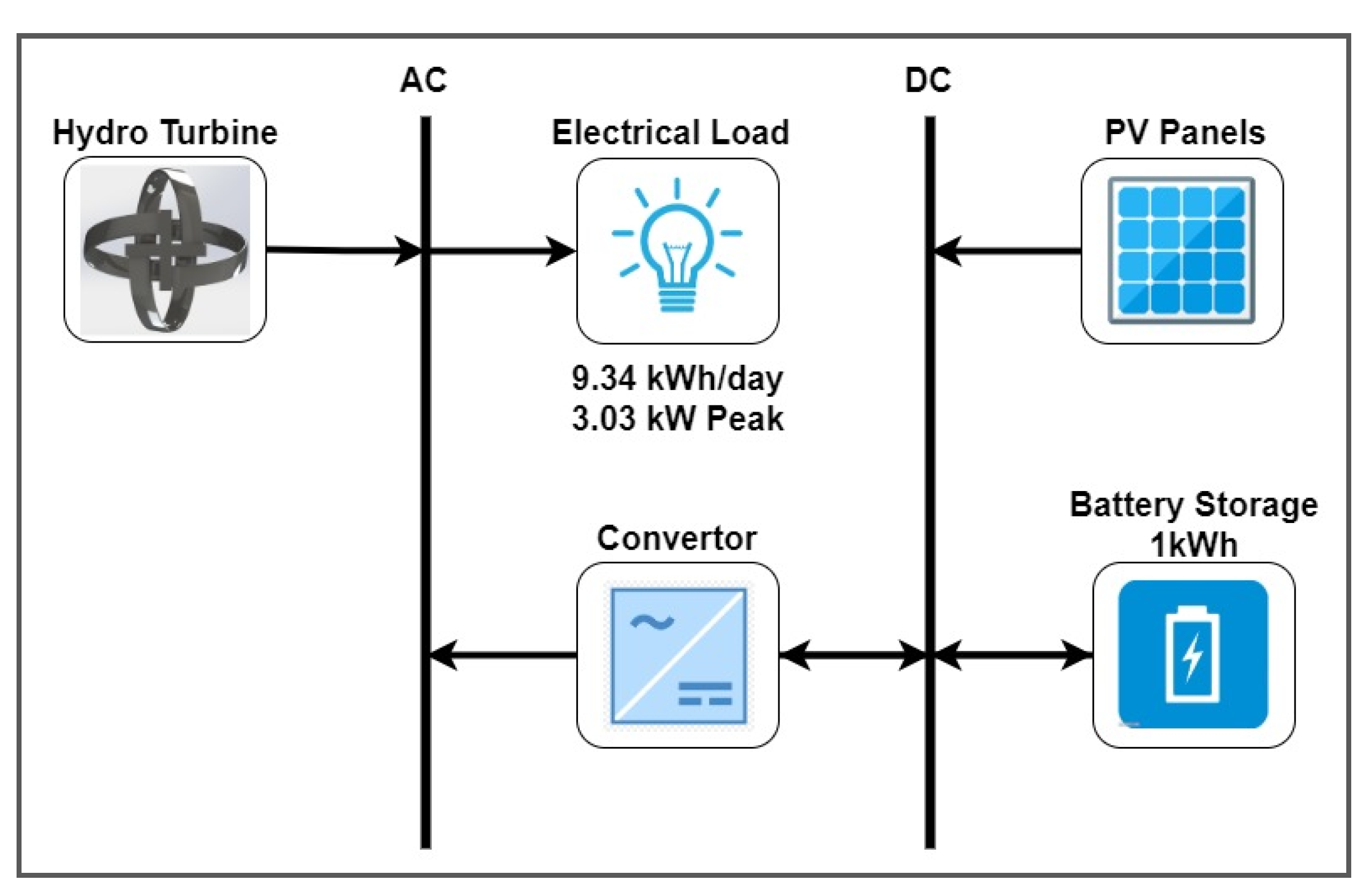
2.2. Microgrid Design
2.3. Optimization
3. Turbine Design
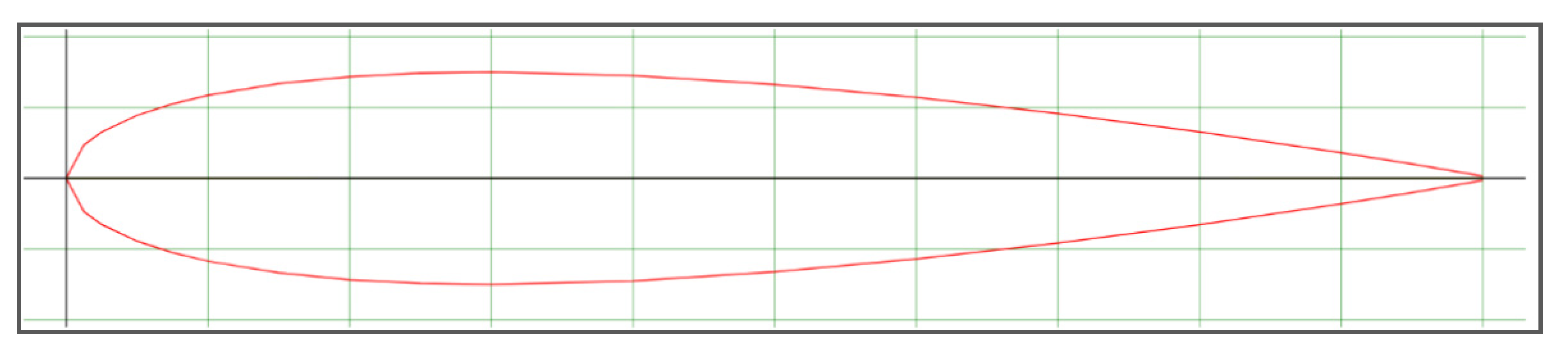
3.1. Blade Profile
3.2. Tip-to-Speed Ratio
3.3. Torque and Power Coefficient
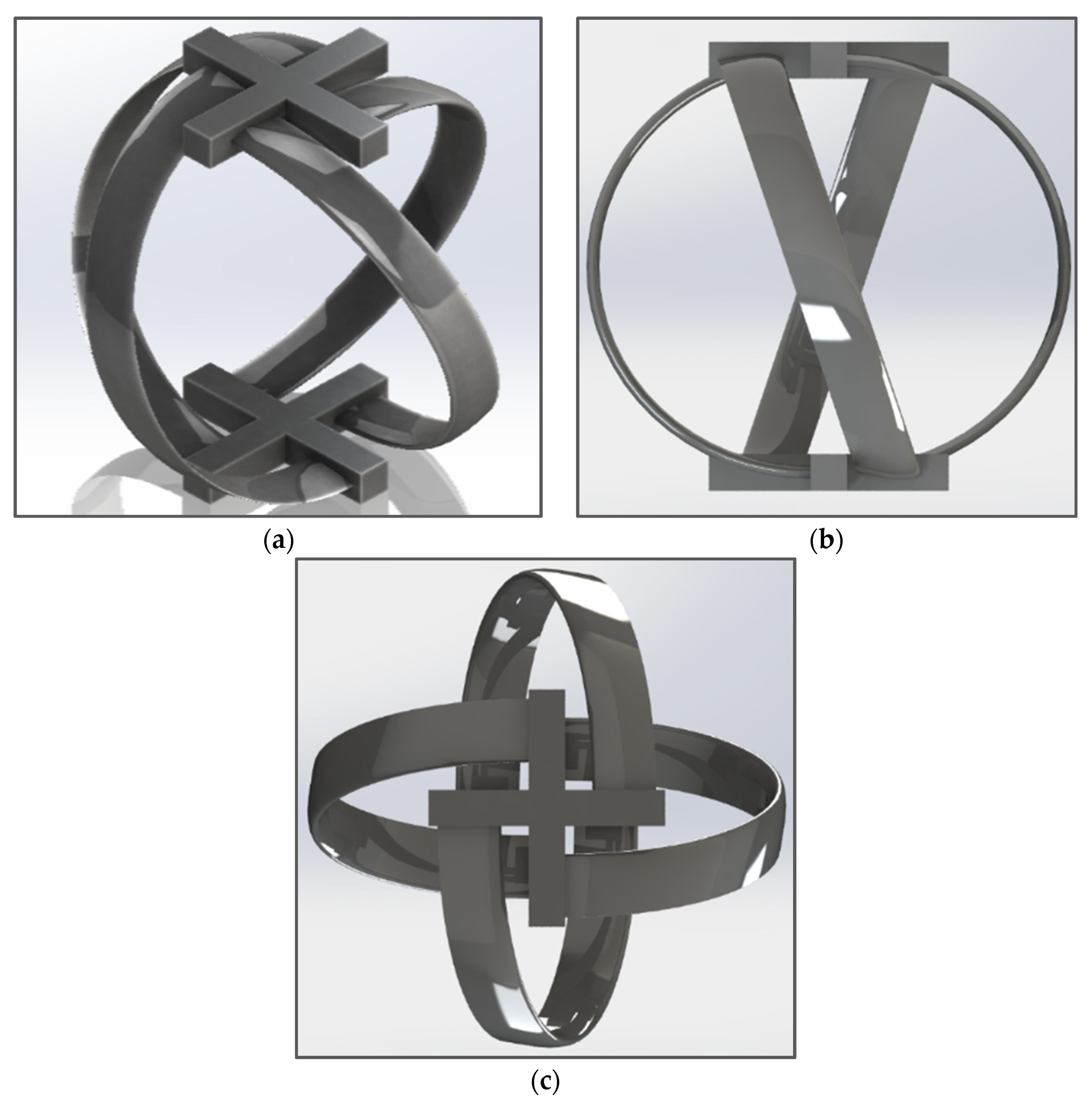
3.4. Final Design
4. CFD Analysis
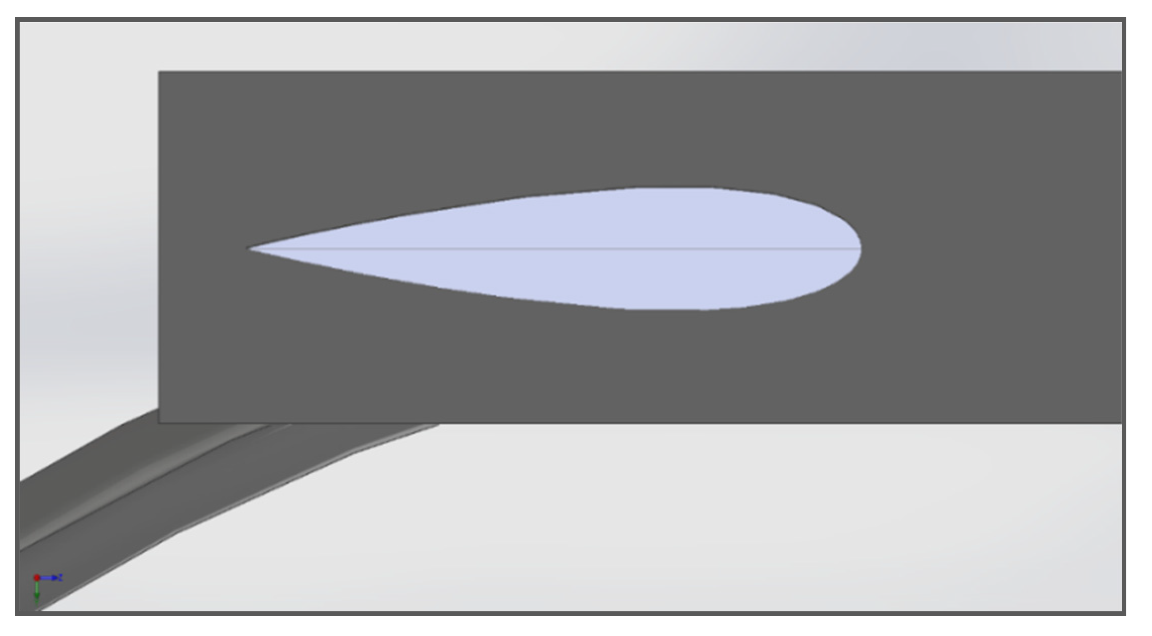
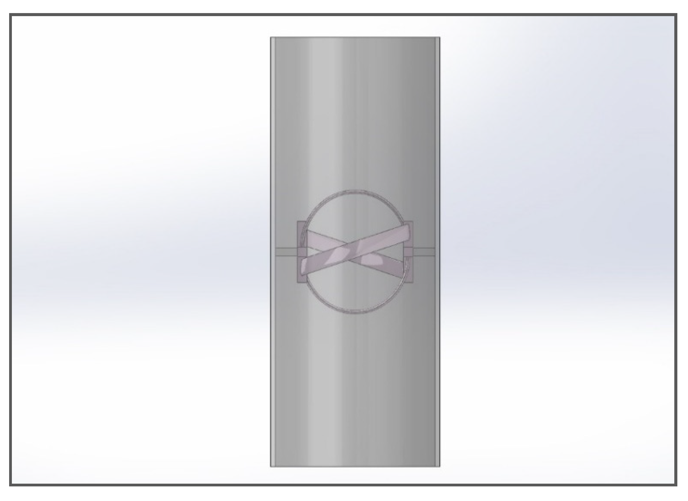
4.1. Turbine Container
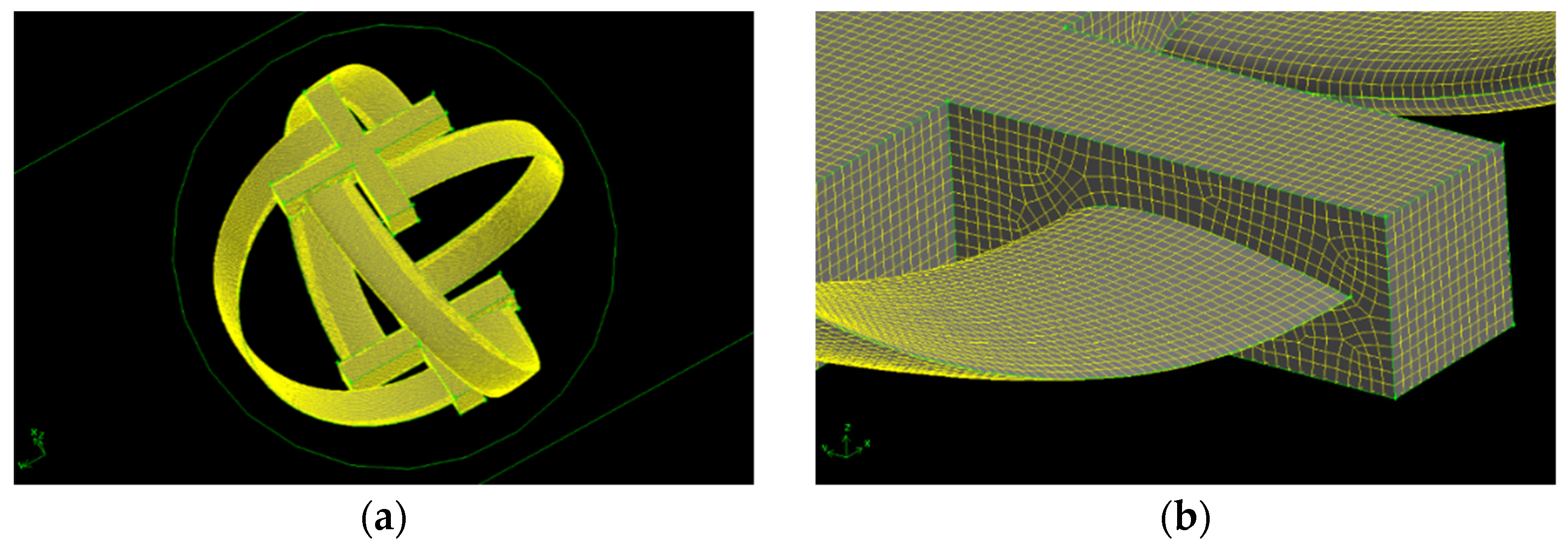
4.2. Meshing
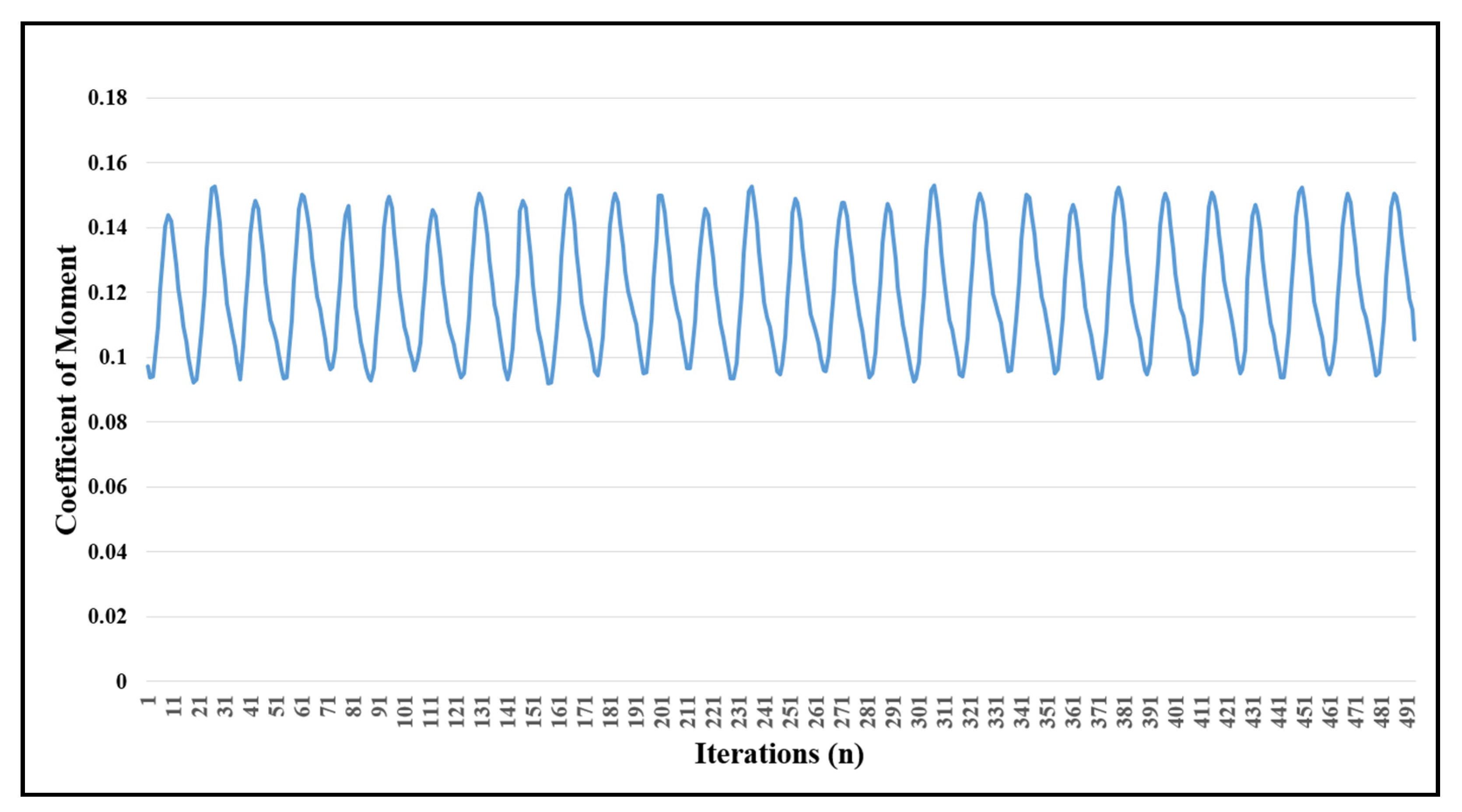
4.3. Numerical Analysis
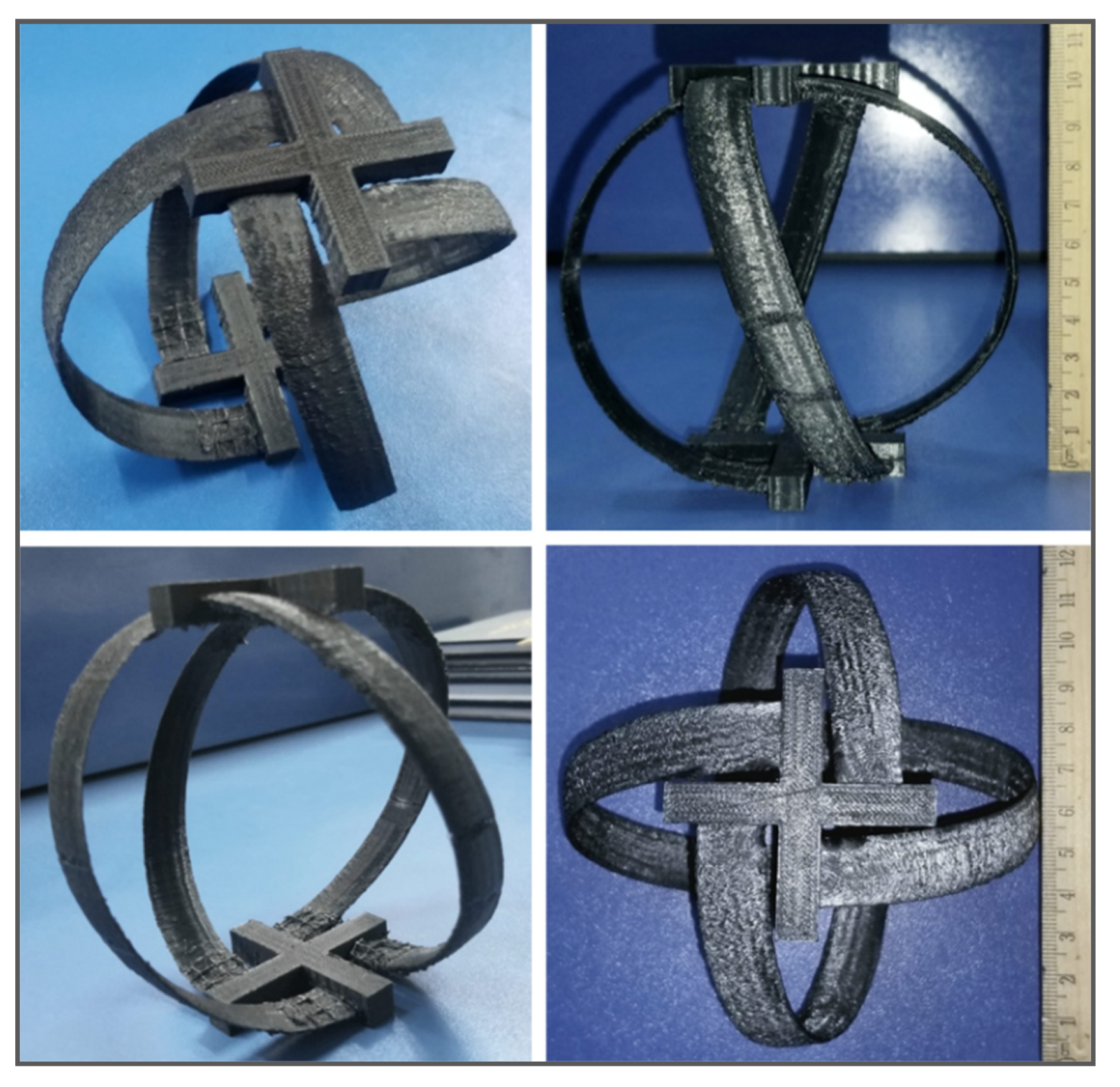
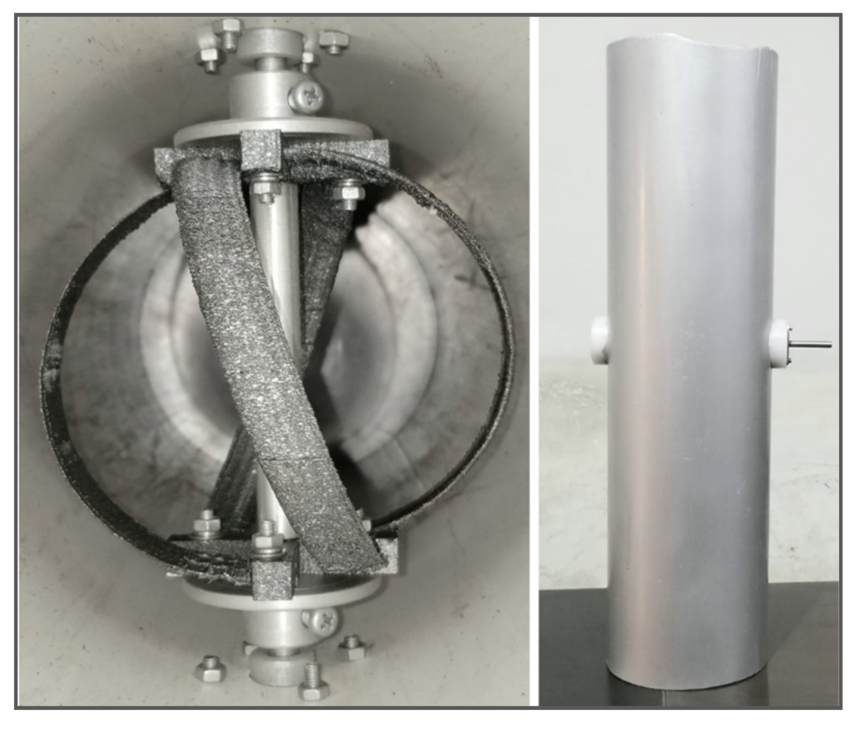
4.4. Hardware Prototype
5. Results and Discussions
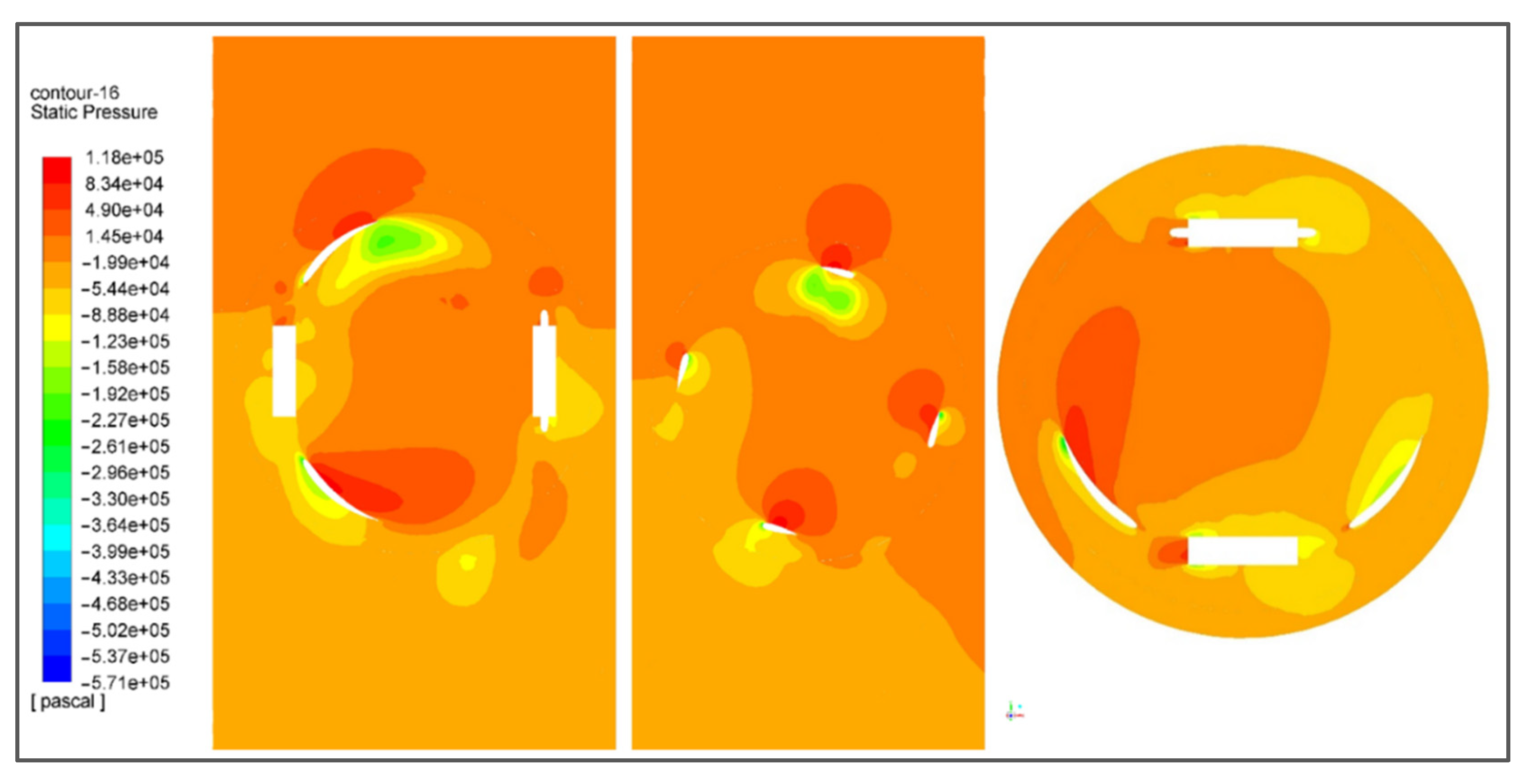
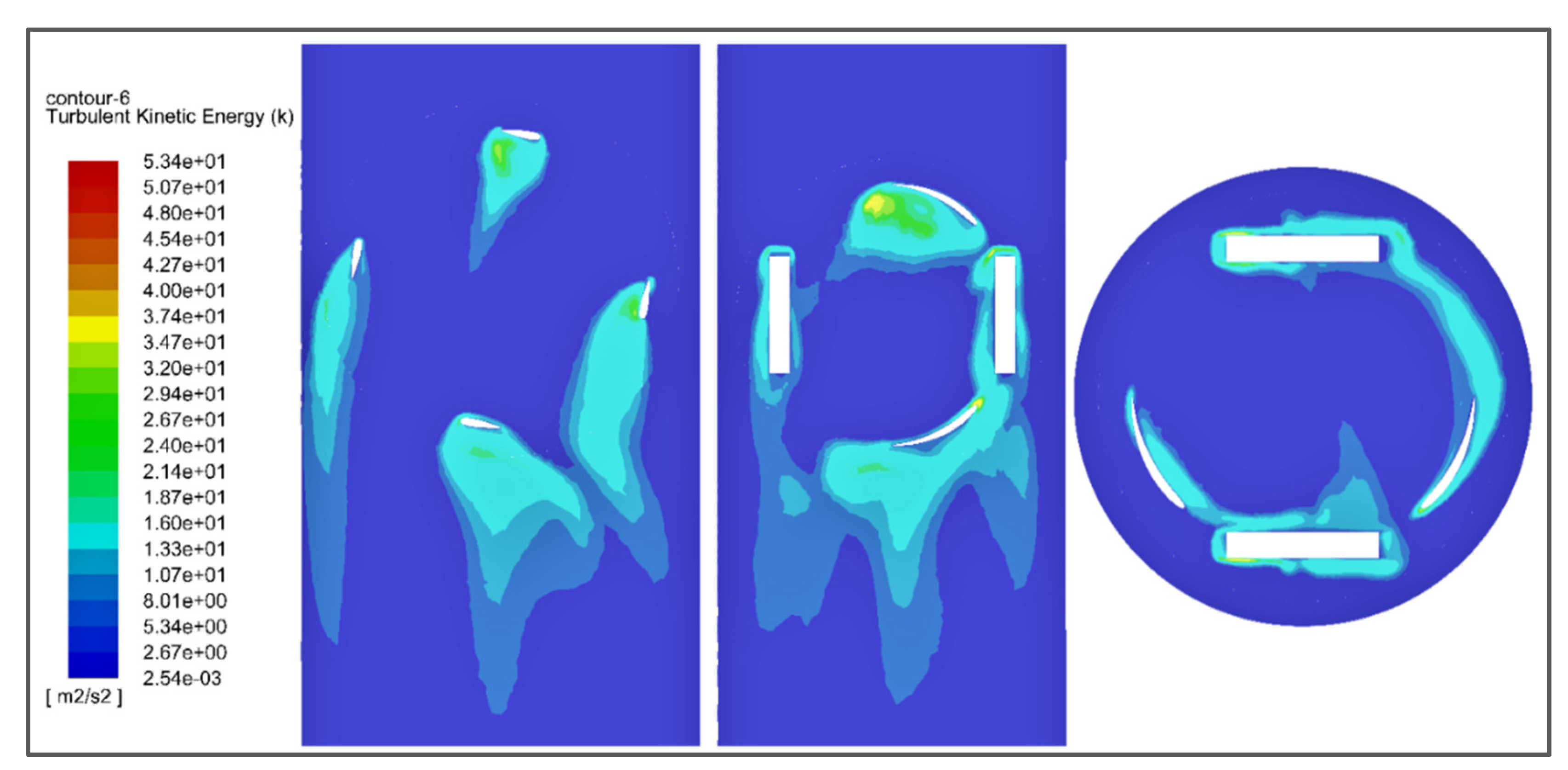
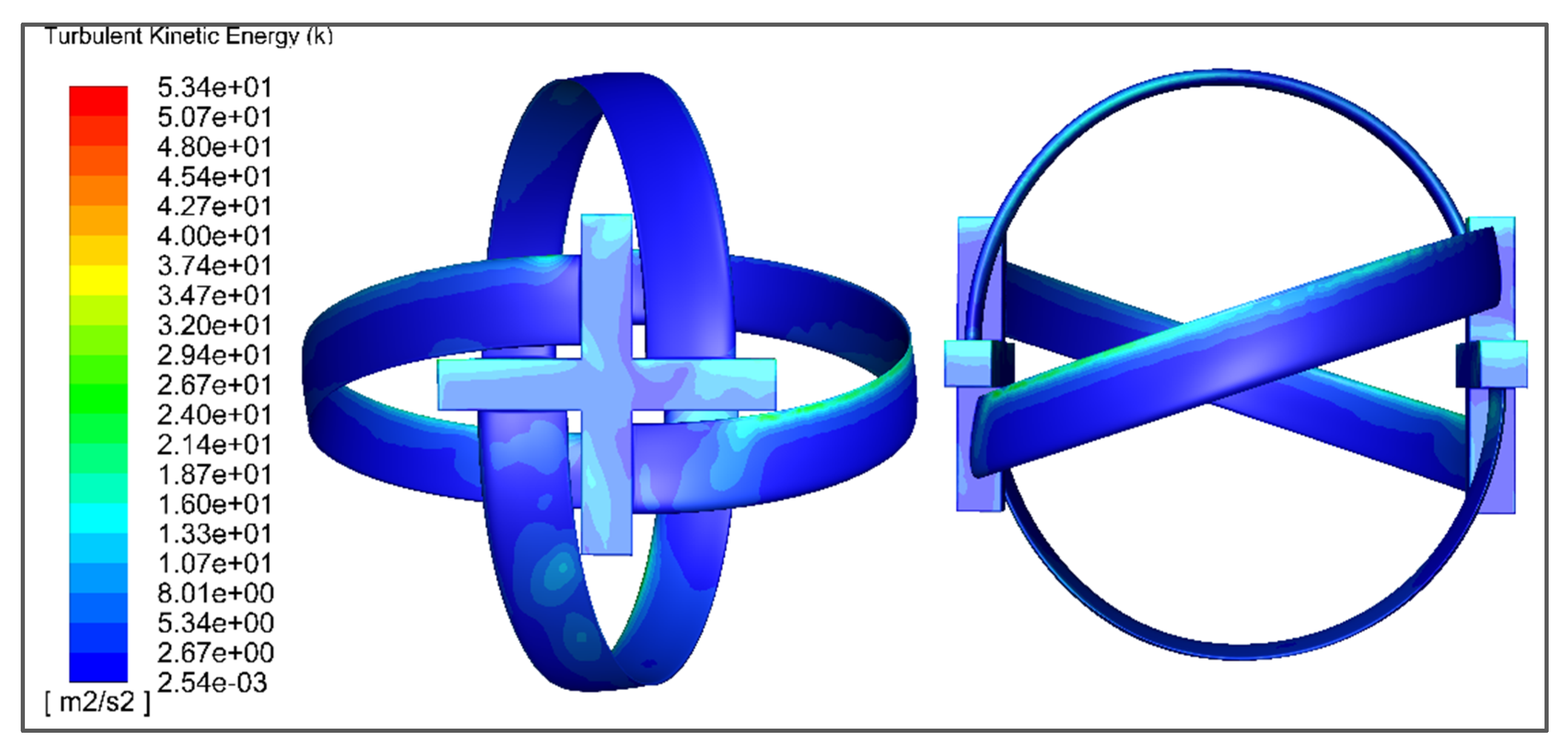
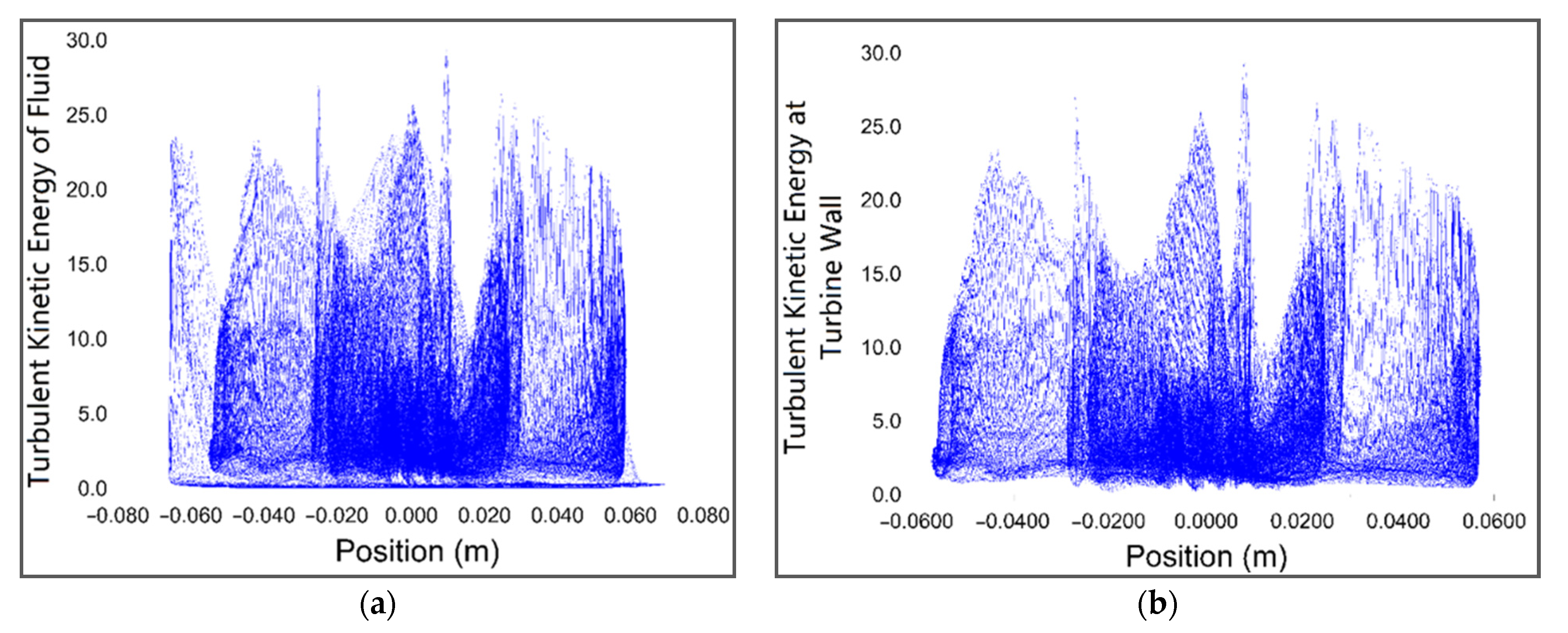
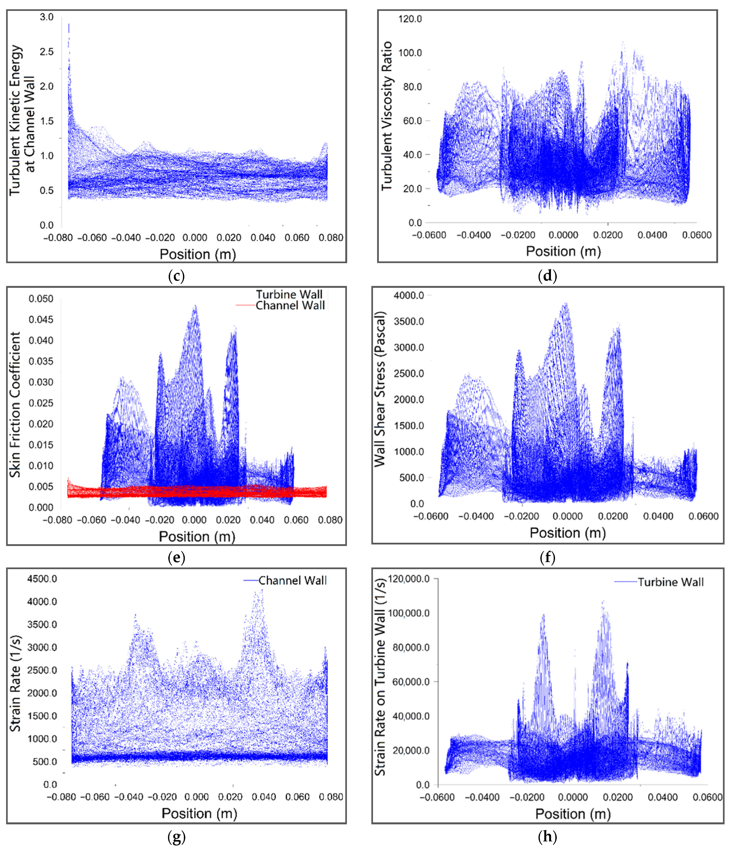
5.1. CFD Results
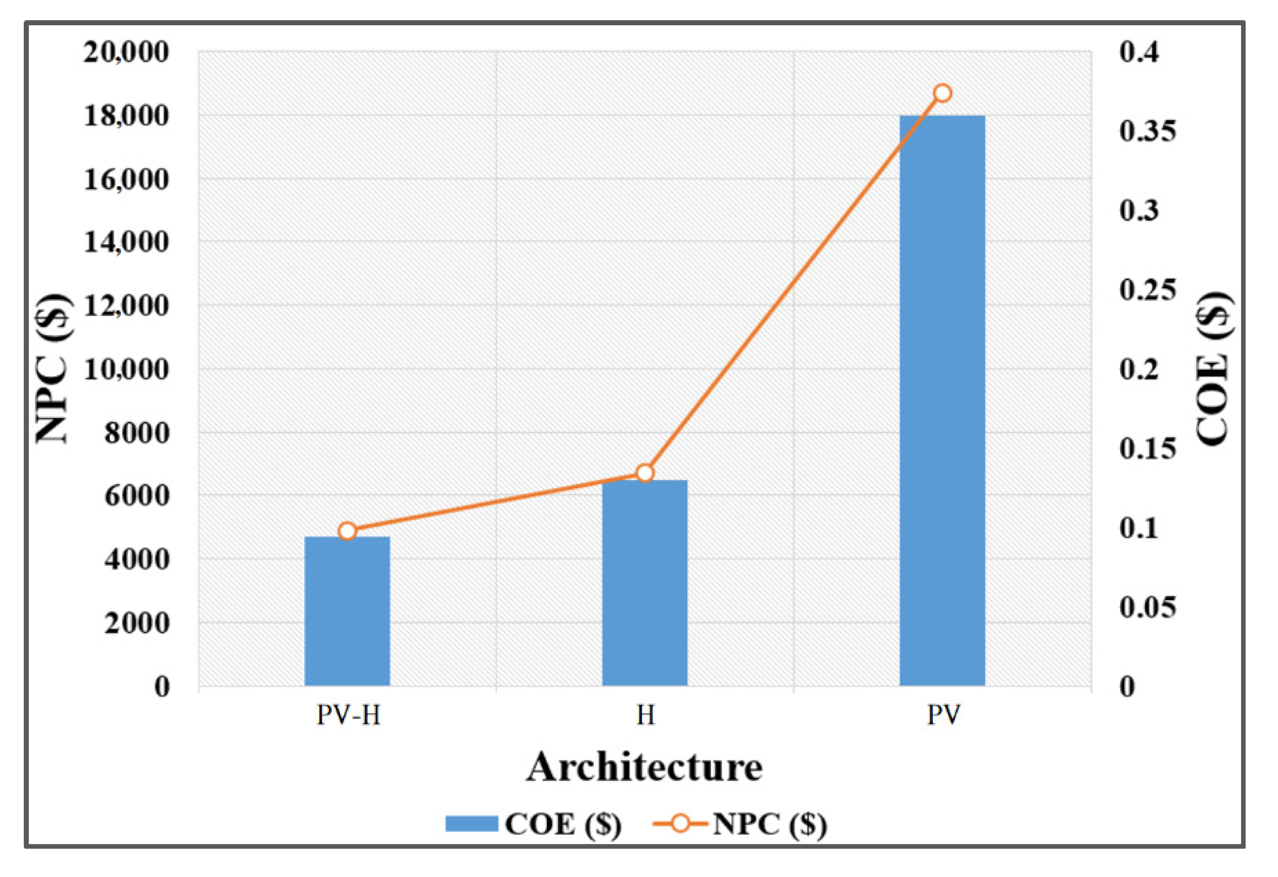
5.2. Techno-Economical Analysis of the nZEB Model
6. Limitations and Future Work
7. Conclusions
Author Contributions
Funding
Institutional Review Board Statement
Informed Consent Statement
Data Availability Statement
Acknowledgments
Conflicts of Interest
Nomenclature
| nZEB | Nearly Zero Energy Building |
| HRES | Hybrid Renewable Energy Systems |
| CFD | Computational Fluid Dynamics |
| ANSYS | Analysis of Systems |
| HOMER | Hybrid Optimization of Multiple Energy Resources |
| DNI | Direct Normal Irradiation |
| IRENA | International Renewable Energy Agency |
| IEA | International Energy Agency |
| PV | Photovoltaic |
| ZEBRA | Zero Energy Building Research Alliance |
| UK | United Kingdom |
| USA | United States of America |
| EMS | Energy Management System |
| MILP | Mixed-Integer Linear Programming |
| NASA | National Aeronautics and Space Administration |
| AC | Alternating Current |
| DC | Direct Current |
| O&M | Operation and Maintenance |
| RMS | Root-Mean-Square |
| COE | Cost of Energy |
| NPC | Net Present Cost |
| BEM | Blade Elemental Momentum |
| NACA | National Advisory Committee for Aeronautics |
| GAMBIT | Geometry and Mesh Building Intelligent Tool |
| 3D | Three Dimensional |
| TKE | Turbulent Kinetic Energy |
| PLA | Poly-Lactic Acid |
| PVA | Poly-Vinyl Alcohol |
| OPEC | Organization of the Petroleum-Exporting Countries |
| Total Annual Cost | |
| Energy Delivered to Load | |
| Energy Delivered to Grid | |
| Capital Recovery Factor | |
| Cross-Sectional Area of Turbine | |
| Interest Rate | |
| Density of Fluid | |
| Resultant Velocity | |
| Velocity of Fluid | |
| Angle of Attack | |
| Tip to Speed Ratio | |
| Angular Speed | |
| Torque Coefficient | |
| Torque | |
| Power Coefficient | |
| TKE Due to Buoyancy | |
| , | Adjustable Constants |
| TKE Due to Velocity Gradients of Fluid | |
| User-Defined Terms | |
| Efficiency | |
| Moment of Turbine | |
| Dynamic Pressure | |
| , αε | Inverse of the Effective Prandtl Numbers |
| Ratio of Compressible Turbulence Due to Fluctuating Dilatation to Overall Dissipation Rate |
References
- IRENA. Renewable Energy Statistics 2020. 2020. Available online: https://www.irena.org/publications/2020/Mar/Renewable-Capacity-Statistics-2020 (accessed on 21 August 2021).
- Newell, R.; Raimi, D.; Villanueva, S.; Prest, B. Global Energy Outlook 2020: Energy Transition or Energy Addition? 2020. Available online: https://media.rff.org/documents/GEO_2020_Report.pdf (accessed on 21 August 2021).
- IEA. Renewables 2020, Paris. 2020. Available online: https://www.iea.org/reports/renewables-2020 (accessed on 21 August 2021).
- Mokhtara, C.; Negrou, B.; Bouferrouk, A.; Yao, Y.; Settou, N.; Ramadan, M. Integrated supply–demand energy management for optimal design of off-grid hybrid renewable energy systems for residential electrification in arid climates. Energy Convers. Manag. 2020, 221, 113192. [Google Scholar] [CrossRef]
- World Energy Council. World Energy Issues Monitor 2020: Decoding New Signals of Change. Issues Monitor. 2020. Available online: https://www.worldenergy.org/publications/entry/issues-monitor-2020-signals-change (accessed on 21 August 2021).
- Feng, W.; Zhang, Q.; Ji, H.; Wang, R.; Zhou, N.; Ye, Q.; Hao, B.; Li, Y.; Luo, D.; Lau, S.S.Y. A review of net zero energy buildings in hot and humid climates: Experience learned from 34 case study buildings. Renew. Sustain. Energy Rev. 2019, 114, 109303. [Google Scholar] [CrossRef]
- European Union Council. Directive 2010/31/Eu of The European Parliament and of The Council of 19 May 2010 on the Energy Performance of Buildings. Off. J. Eur. Union 2010, 153, 13–35. Available online: http://data.europa.eu/eli/dir/2010/31/oj (accessed on 30 October 2021).
- Kewat, S.; Singh, B.; Hussain, I. Power management in PV—Battery-hydro based standalone microgrid. IET Renew. Power Gener. 2018, 12, 391–398. [Google Scholar] [CrossRef]
- Meshram, S.; Agnihotri, G.; Gupta, S. Performance Analysis of Grid Integrated Hydro and Solar Based Hybrid Systems. Adv. Power Electron. 2013, 2013, 697049. [Google Scholar] [CrossRef]
- Khan, M.A.; Zeb, K.; Uddin, W.; Sathishkumar, P.; Ali, M.U.; Hussain, S.; Ishfaq, M.; Himanshu; Subramanian, A.; Kim, H.-J. Design of a Building-Integrated Photovoltaic System with a Novel Bi-Reflector PV System (BRPVS) and Optimal Control Mechanism: An Experimental Study. Electronics 2018, 7, 119. [Google Scholar] [CrossRef] [Green Version]
- Sun, Y.; Ma, R.; Chen, J.; Xu, T. Heuristic optimization for grid-interactive net-zero energy building design through the glowworm swarm algorithm. Energy Build. 2020, 208, 109644. [Google Scholar] [CrossRef]
- Li, H.; Wang, S. Coordinated optimal design of zero/low energy buildings and their energy systems based on multi-stage design optimization. Energy 2019, 189, 116202. [Google Scholar] [CrossRef]
- Shin, M.; Baltazar, J.-C.; Haberl, J.S.; Frazier, E.; Lynn, B. Evaluation of the energy performance of a net zero energy building in a hot and humid climate. Energy Build. 2019, 204, 109531. [Google Scholar] [CrossRef]
- Lagrange, A.; de Simón-Martín, M.; González-Martínez, A.; Bracco, S.; Rosales-Asensio, E. Sustainable microgrids with energy storage as a means to increase power resilience in critical facilities: An application to a hospital. Int. J. Electr. Power Energy Syst. 2020, 119, 105865. [Google Scholar] [CrossRef]
- Moser, A.; Muschick, D.; Gölles, M.; Nageler, P.; Schranzhofer, H.; Mach, T.; Tugores, C.R.; Leusbrock, I.; Stark, S.; Lackner, F.; et al. A MILP-based modular energy management system for urban multi-energy systems: Performance and sensitivity analysis. Appl. Energy 2020, 261, 114342. [Google Scholar] [CrossRef]
- Elkadeem, M.; Wang, S.; Sharshir, S.; Atia, E.G. Feasibility analysis and techno-economic design of grid-isolated hybrid renewable energy system for electrification of agriculture and irrigation area: A case study in Dongola, Sudan. Energy Convers. Manag. 2019, 196, 1453–1478. [Google Scholar] [CrossRef]
- Spitalny, L.; Unger, D.; Teuwsen, J.; Liebenau, V.; Myrzik, J.M.A.; Van Reeth, B. Effectiveness of a building energy management system for the integration of net zero energy buildings into the grid and for providing tertiary control reserve. In Proceedings of the 2013 IEEE Grenoble Conference, Grenoble, France, 16–20 June 2013; IEEE: Piscataway, NJ, USA, 2013; pp. 1–6. [Google Scholar] [CrossRef]
- Chabaud, A.; Eynard, J.; Grieu, S. A new approach to energy resources management in a grid-connected building equipped with energy production and storage systems: A case study in the south of France. Energy Build. 2015, 99, 9–31. [Google Scholar] [CrossRef]
- Querikiol, E.M.; Taboada, E.B. Performance Evaluation of a Micro Off-Grid Solar Energy Generator for Islandic Agricultural Farm Operations Using HOMER. J. Renew. Energy 2018, 2018, 2828173. [Google Scholar] [CrossRef] [Green Version]
- Suresh, V.; Muralidhar, M.; Kiranmayi, R. Modelling and optimization of an off-grid hybrid renewable energy system for electrification in a rural areas. Energy Rep. 2020, 6, 594–604. [Google Scholar] [CrossRef]
- Mayer, M.J.; Szilágyi, A.; Gróf, G. Environmental and economic multi-objective optimization of a household level hybrid renewable energy system by genetic algorithm. Appl. Energy 2020, 269, 115058. [Google Scholar] [CrossRef]
- Huang, Z.; Lu, Y.; Wei, M.; Liu, J. Performance analysis of optimal designed hybrid energy systems for grid-connected nearly/net zero energy buildings. Energy 2017, 141, 1795–1809. [Google Scholar] [CrossRef]
- Harkouss, F.; Fardoun, F.; Biwole, P.H. Optimal design of renewable energy solution sets for net zero energy buildings. Energy 2019, 179, 1155–1175. [Google Scholar] [CrossRef]
- Du, J.; Yang, H.; Shen, Z.; Chen, J. Micro hydro power generation from water supply system in high rise buildings using pump as turbines. Energy 2017, 137, 431–440. [Google Scholar] [CrossRef]
- Paish, O. Small hydro power: Technology and current status. Renew. Sustain. Energy Rev. 2002, 6, 537–556. [Google Scholar] [CrossRef]
- Mabrouki, I.; Driss, Z.; Abid, M.S. Experimental Investigation of the Height Effect of Water Savonius Rotors. Int. J. Mech. Appl. 2014, 4, 8–12. [Google Scholar] [CrossRef]
- Li, Y.; Calisal, S.M. Three-dimensional effects and arm effects on modeling a vertical axis tidal current turbine. Renew. Energy 2010, 35, 2325–2334. [Google Scholar] [CrossRef]
- Golecha, K.; Eldho, T.I.; Prabhu, S.V. Study on the Interaction between Two Hydrokinetic Savonius Turbines. Int. J. Rotating Mach. 2012, 2012, 581658. [Google Scholar] [CrossRef]
- Tummala, A.; Velamati, R.K.; Sinha, D.K.; Indraja, V.; Krishna, V.H. A review on small scale wind turbines. Renew. Sustain. Energy Rev. 2016, 56, 1351–1371. [Google Scholar] [CrossRef]
- Gorlov, A.M. Unidirectional Helical Reaction Turbine Operable under Reversible Fluid Flow for Power Systems. U.S. Patent 5,451,137, 19 September 1995. [Google Scholar]
- Golecha, K.; Eldho, T.; Prabhu, S. Influence of the deflector plate on the performance of modified Savonius water turbine. Appl. Energy 2011, 88, 3207–3217. [Google Scholar] [CrossRef]
- Bianchini, A.; Balduzzi, F.; Bachant, P.; Ferrara, G.; Ferrari, L. Effectiveness of two-dimensional CFD simulations for Darrieus VAWTs: A combined numerical and experimental assessment. Energy Convers. Manag. 2017, 136, 318–328. [Google Scholar] [CrossRef]
- Bouzaher, M.T.; Hadid, M. Numerical Investigation of a Vertical Axis Tidal Turbine with Deforming Blades. Arab. J. Sci. Eng. 2017, 42, 2167–2178. [Google Scholar] [CrossRef]
- Yang, B.; Lawn, C. Fluid dynamic performance of a vertical axis turbine for tidal currents. Renew. Energy 2011, 36, 3355–3366. [Google Scholar] [CrossRef]
- Bachant, P.; Wosnik, M. Performance measurements of cylindrical- and spherical-helical cross-flow marine hydrokinetic turbines, with estimates of exergy efficiency. Renew. Energy 2015, 74, 318–325. [Google Scholar] [CrossRef]
- Derakhshan, S.; Ashoori, M.; Salemi, A. Experimental and numerical study of a vertical axis tidal turbine performance. Ocean Eng. 2017, 137, 59–67. [Google Scholar] [CrossRef] [Green Version]
- Velasco, D.; Mejia, O.D.L.; Lain, S. Numerical simulations of active flow control with synthetic jets in a Darrieus turbine. Renew. Energy 2017, 113, 129–140. [Google Scholar] [CrossRef]
- Elbatran, A.H.; Ahmed, Y.M.; Shehata, A.S. Performance study of ducted nozzle Savonius water turbine, comparison with conventional Savonius turbine. Energy 2017, 134, 566–584. [Google Scholar] [CrossRef]
- Shimokawa, K.; Furukawa, A.; Okuma, K.; Matsushita, D.; Watanabe, S. Experimental study on simplification of Darrieus-type hydro turbine with inlet nozzle for extra-low head hydropower utilization. Renew. Energy 2012, 41, 376–382. [Google Scholar] [CrossRef]
- Sahim, K.; Santoso, D.; Radentan, A. Performance of Combined Water Turbine with Semielliptic Section of the Savonius Rotor. Int. J. Rotating Mach. 2013, 2013, 985943. [Google Scholar] [CrossRef] [Green Version]
- Sarma, N.; Biswas, A.; Misra, R. Experimental and computational evaluation of Savonius hydrokinetic turbine for low velocity condition with comparison to Savonius wind turbine at the same input power. Energy Convers. Manag. 2014, 83, 88–98. [Google Scholar] [CrossRef]
- Mohamed, A.B.; Bear, C.; Bear, M.; Korobenko, A. Performance analysis of two vertical-axis hydrokinetic turbines using variational multiscale method. Comput. Fluids 2020, 200, 104432. [Google Scholar] [CrossRef]
- Payambarpour, S.A.; Najafi, A.F.; Magagnato, F. Investigation of deflector geometry and turbine aspect ratio effect on 3D modified in-pipe hydro Savonius turbine: Parametric study. Renew. Energy 2020, 148, 44–59. [Google Scholar] [CrossRef]
- Nishi, Y.; Yahagi, Y.; Okazaki, T.; Inagaki, T. Effect of flow rate on performance and flow field of an undershot cross-flow water turbine. Renew. Energy 2019, 149, 409–423. [Google Scholar] [CrossRef]
- Shahsavarifard, M.; Bibeau, E.L. Performance characteristics of shrouded horizontal axis hydrokinetic turbines in yawed conditions. Ocean Eng. 2020, 197, 106916. [Google Scholar] [CrossRef]
- Ansarifard, N.; Kianejad, S.; Fleming, A.; Henderson, A.; Chai, S. Design optimization of a purely radial turbine for operation in the inhalation mode of an oscillating water column. Renew. Energy 2020, 152, 540–556. [Google Scholar] [CrossRef]
- Fox, R.W.; McDonald, A.T.; Mitchell, J.W. Fox and McDonald’s Introduction to Fluid Mechanics; John Wiley & Sons: Hoboken, NJ, USA, 2020. [Google Scholar]
- Batchelor, C.K.; Batchelor, G.K. An Introduction to Fluid Dynamics; Cambridge University Press: Cambridge, UK, 2000. [Google Scholar]
- Khan, M.A.; Aziz, M.S.; Khan, A.; Zeb, K.; Uddin, W.; Ishfaq, M. An Optimized Off-gird Renewable AC/DC Microgrid for Remote Communities of Pakistan. In Proceedings of the 2019 International Conference on Electrical, Communication, and Computer Engineering (ICECCE), Swat, Pakistan, 24–25 July 2019; pp. 1–6. [Google Scholar] [CrossRef]
- Zhou, J.H.; Ge, X.H.; Zhang, X.S.; Gao, X.Q.; Liu, Y. Stability simulation of a MW-scale PV-small hydro autonomous hybrid system. In Proceedings of the 2013 IEEE Power & Energy Society General Meeting, Vancouver, BC, Canada, 21–25 July 2013; IEEE: Piscataway, NJ, USA, 2013; pp. 1–5. [Google Scholar] [CrossRef]
- NACA 0015 (naca0015-il). Available online: http://airfoiltools.com/airfoil/details?airfoil=naca0015-il (accessed on 21 August 2021).
- Zhou, T.; Rempfer, D. Numerical study of detailed flow field and performance of Savonius wind turbines. Renew. Energy 2013, 51, 373–381. [Google Scholar] [CrossRef]
- McLean, D. Understanding Aerodynamics; John Wiley & Sons, Ltd.: Chichester, UK, 2012. [Google Scholar]
- Mosbahi, M.; Ayadi, A.; Mabrouki, I.; Driss, Z.; Tucciarelli, T.; Abid, M.S. Effect of the Converging Pipe on the Performance of a Lucid Spherical Rotor. Arab. J. Sci. Eng. 2019, 44, 1583–1600. [Google Scholar] [CrossRef]


| Parameter | Specification |
|---|---|
| Panel Type | Flat Plate |
| Capacity | 1 kW |
| Capital Cost | $1000 |
| O&M Cost | $10/Year |
| Lifetime | 25 Years |
| Derating Factor | 80% |
| Ground Reflectance | 20% |
| Nominal Operating Cell Temperature | 47 °C |
| Temperature Effects on Power | −0.500%/°C |
| Efficiency at Standard Test Conditions | 13% |
| Parameter | Specification |
|---|---|
| Nominal Voltage | 12 V |
| Nominal Capacity | 1 kWh |
| Maximum Capacity | 83.4 Ah |
| Capacity Ratio | 0.403 |
| Rate Constant | 0.827/h |
| Roundtrip efficiency | 80% |
| Maximum Charge Current | 16.7 A |
| Maximum Discharge Current | 24.3 A |
| Maximum Charge Rate | 1 A/Ah |
| Parameters | Specification |
|---|---|
| Torque (T) | 6.417 Nm |
| Angular Velocity () | 26.18 rad/s |
| Tip to Speed Ratio () | 0.1195 |
| Blades (B) | 4 |
| Height (H) | 107.14 mm |
| Diameter (D) | 115.6 mm |
| Fluid Speed () | 12.66 m/s |
| Helix Angle (δ) | 71.45° |
| Chord Length (C) | 15.40 mm |
| Blade Length | 160.08 mm |
| Hydrofoil Profile | NACA 0015 |
| Parameter | Specification |
|---|---|
| Fill Density | 100% |
| Speed | 100 mm/sec |
| Layer Height | 0.1 mm |
| Nozzle Temperature | 210 °C |
| Bed Temperature | 50 °C |
| Nozzle Diameter | 0.4 mm |
| Architecture | PV-H | H | PV |
|---|---|---|---|
| PV (kW) | 1.06556 | - | 8.09370 |
| LA Battery | 6 | 11 | 17 |
| Hydroelectric (kW) | 1.9855 | 1.9855 | - |
| Converter (kW) | 1.4848 | 2.1875 | 5.4926 |
| NPC ($) | 4902.807 | 6692.714 | 18,694.98 |
| COE ($) | 0.09418 | 0.12964 | 0.35960 |
| Operating Cost ($/yr) | 190.2029 | 336.1491 | 491.3187 |
| Initial Capital ($) | 3411.02 | 4056.25 | 14,841.5 |
| PV Capital Cost ($) | 1065.561 | - | 8093.708 |
| PV Output (kWh/yr) | 1867.62 | - | 14,185.92 |
| Component | Capital ($) | Replacement ($) | O&M ($) | Salvage ($) | Total ($) |
|---|---|---|---|---|---|
| Hydro-Turbine | 600.0 | 324.56 | 57 | −1.76 | 1079.66 |
| 1 kWh Lead Acid | 211 | 124.85 | 8 | −19.51 | 363.93 |
| PV System | 1065.0 | 0 | 3.57 | 0.00 | 1148.57 |
| System Converter | 445.46 | 81.38 | 0 | −8.73 | 518.11 |
Publisher’s Note: MDPI stays neutral with regard to jurisdictional claims in published maps and institutional affiliations. |
© 2021 by the authors. Licensee MDPI, Basel, Switzerland. This article is an open access article distributed under the terms and conditions of the Creative Commons Attribution (CC BY) license (https://creativecommons.org/licenses/by/4.0/).
Share and Cite
Aziz, M.S.; Khan, M.A.; Jamil, H.; Jamil, F.; Chursin, A.; Kim, D.-H. Design and Analysis of In-Pipe Hydro-Turbine for an Optimized Nearly Zero Energy Building. Sensors 2021, 21, 8154. https://doi.org/10.3390/s21238154
Aziz MS, Khan MA, Jamil H, Jamil F, Chursin A, Kim D-H. Design and Analysis of In-Pipe Hydro-Turbine for an Optimized Nearly Zero Energy Building. Sensors. 2021; 21(23):8154. https://doi.org/10.3390/s21238154
Chicago/Turabian StyleAziz, Muhammad Shahbaz, Muhammad Adil Khan, Harun Jamil, Faisal Jamil, Alexander Chursin, and Do-Hyeun Kim. 2021. "Design and Analysis of In-Pipe Hydro-Turbine for an Optimized Nearly Zero Energy Building" Sensors 21, no. 23: 8154. https://doi.org/10.3390/s21238154
APA StyleAziz, M. S., Khan, M. A., Jamil, H., Jamil, F., Chursin, A., & Kim, D.-H. (2021). Design and Analysis of In-Pipe Hydro-Turbine for an Optimized Nearly Zero Energy Building. Sensors, 21(23), 8154. https://doi.org/10.3390/s21238154