
Studies on Three-Dimensional (3D) Accuracy Optimization and Repeatability of UAV in Complex Pit-Rim Landforms As Assisted by Oblique Imaging and RTK Positioning


Abstract
:1. Introduction
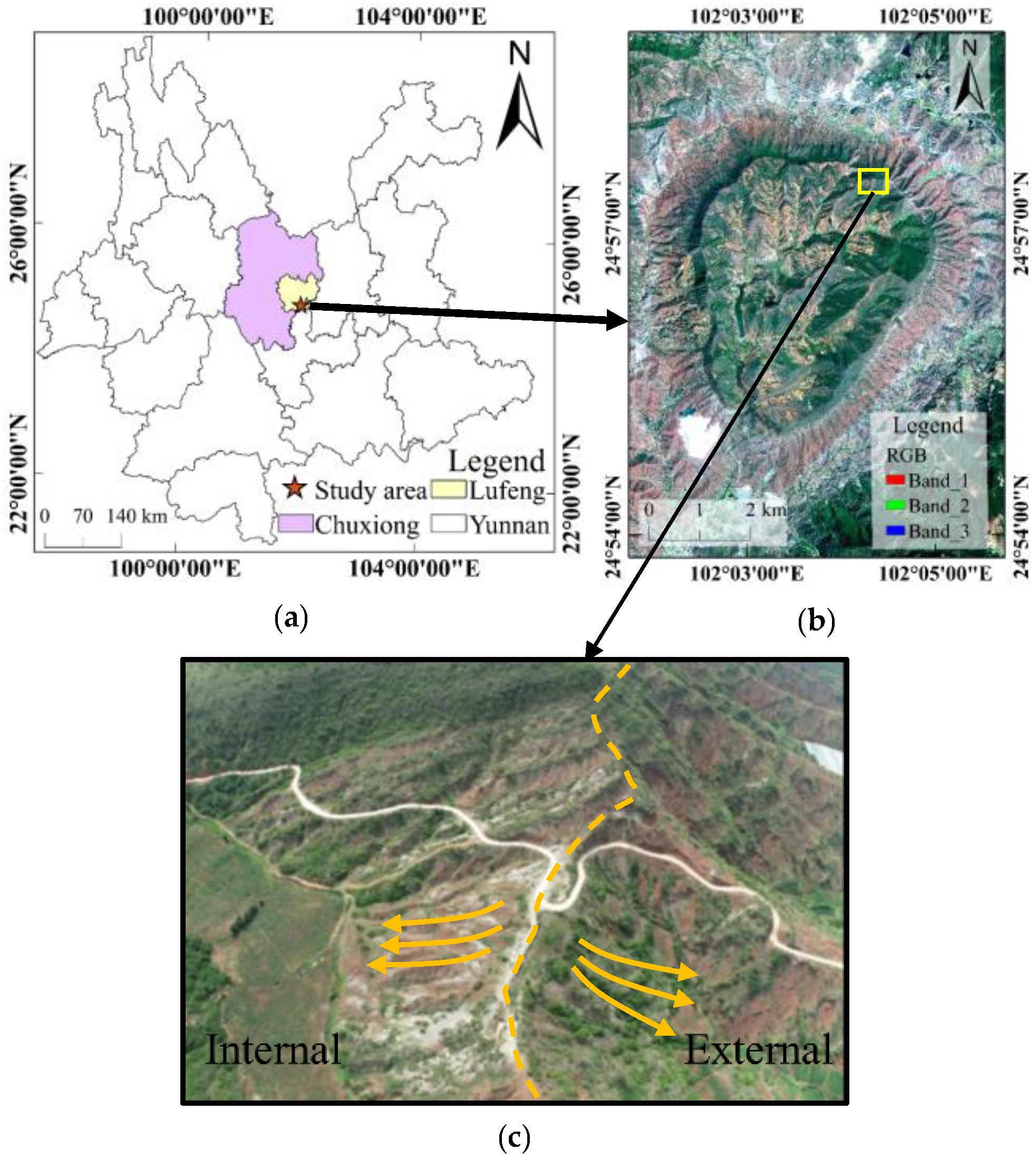
2. Study Area
3. Material and Methods
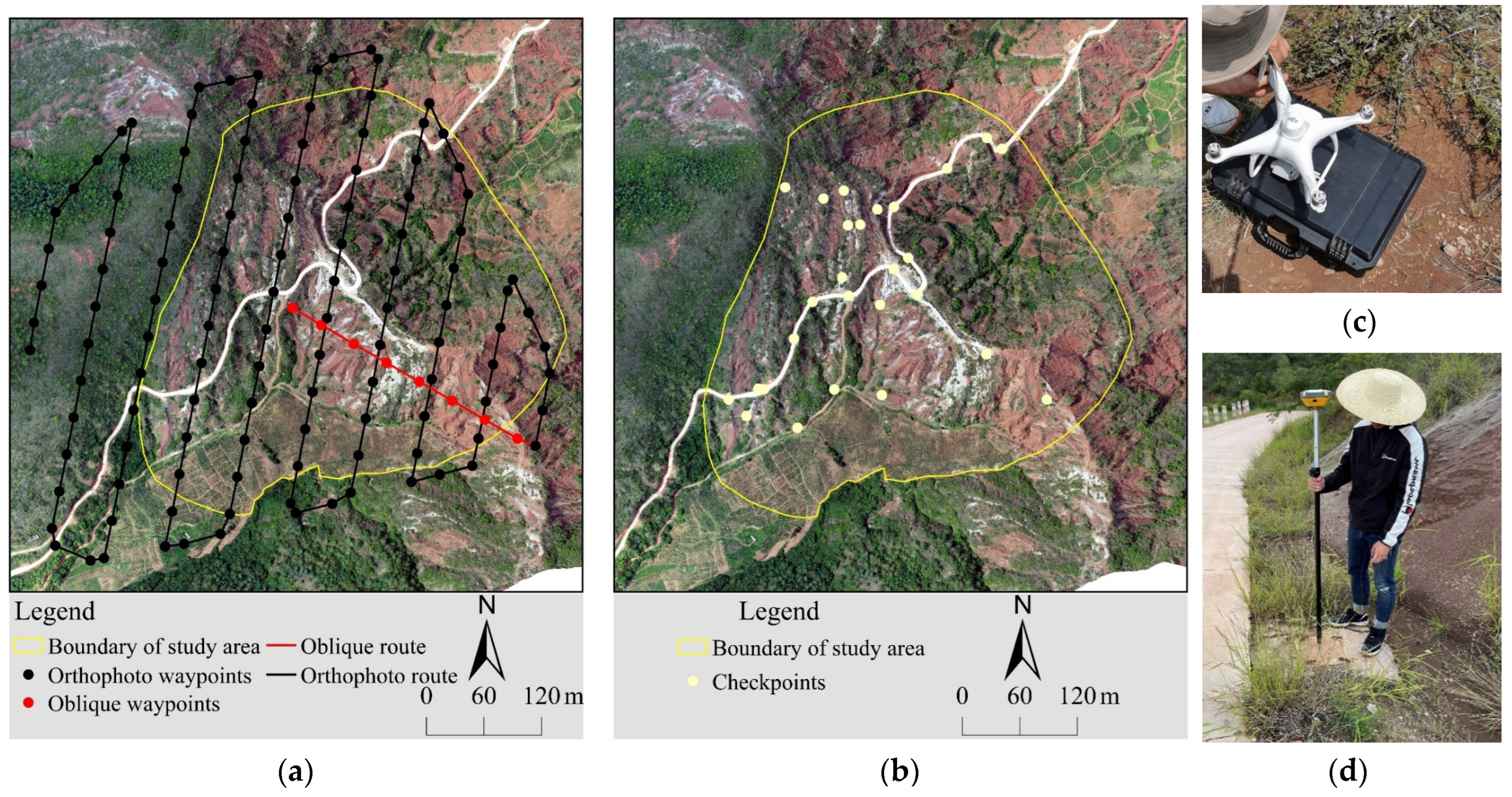
3.1. Data Acquisition
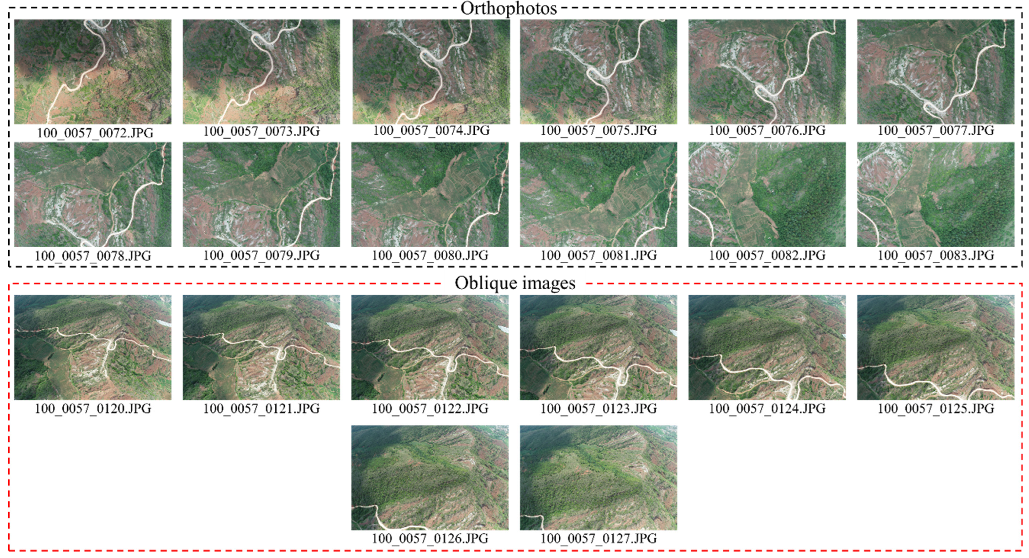
3.1.1. UAV Images Collection
3.1.2. Checkpoint Acquisition
3.2. 3D Scene Construction Based on SfM-MVS
3.3. Accuracy Assessment Methods
3.3.1. 3D scene Absolute Accuracy Assessment
3.3.2. Internal and External Precision Assessment
4. Results and Analysis
4.1. 3D Scene Absolute Accuracy Analysis
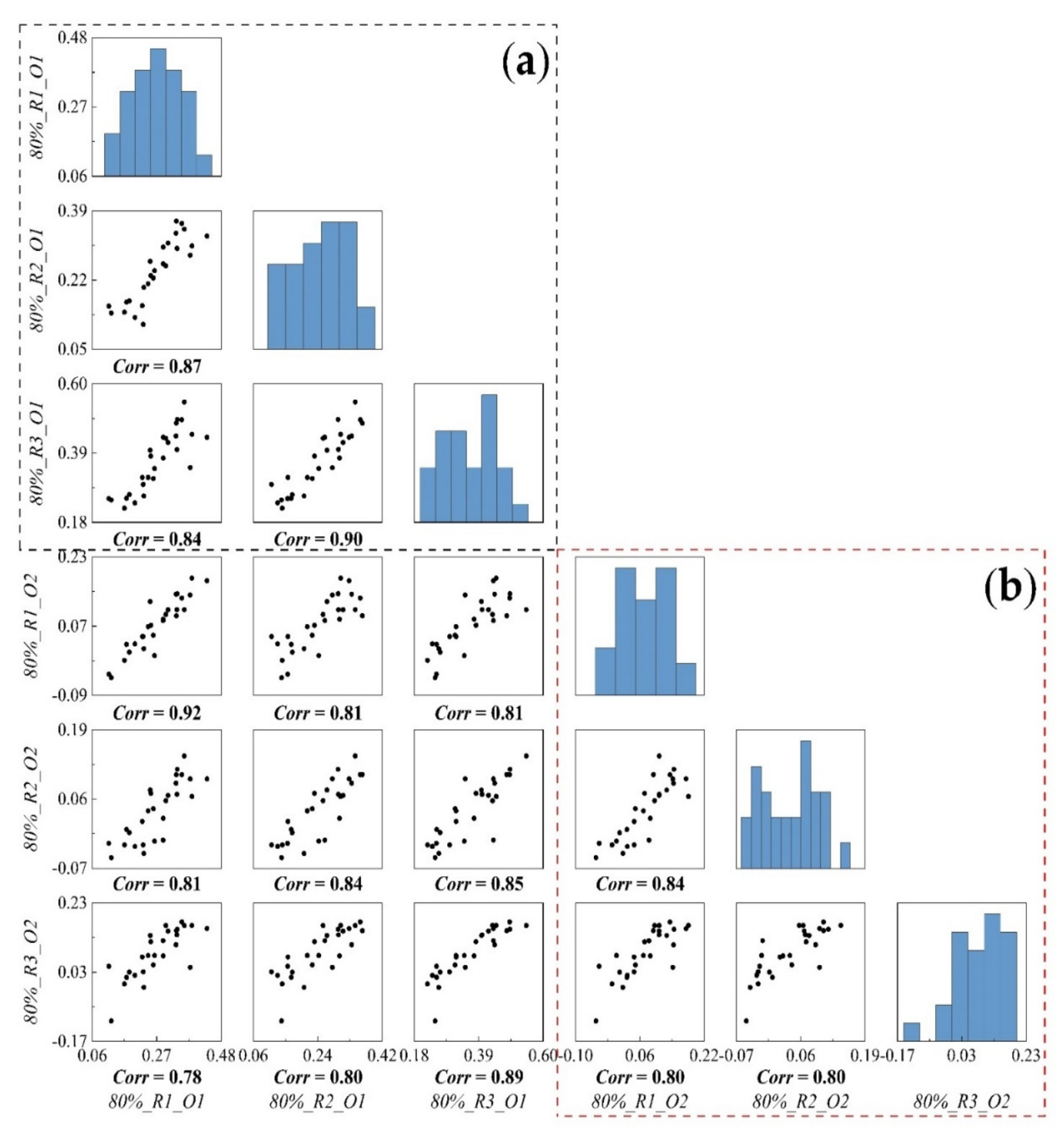
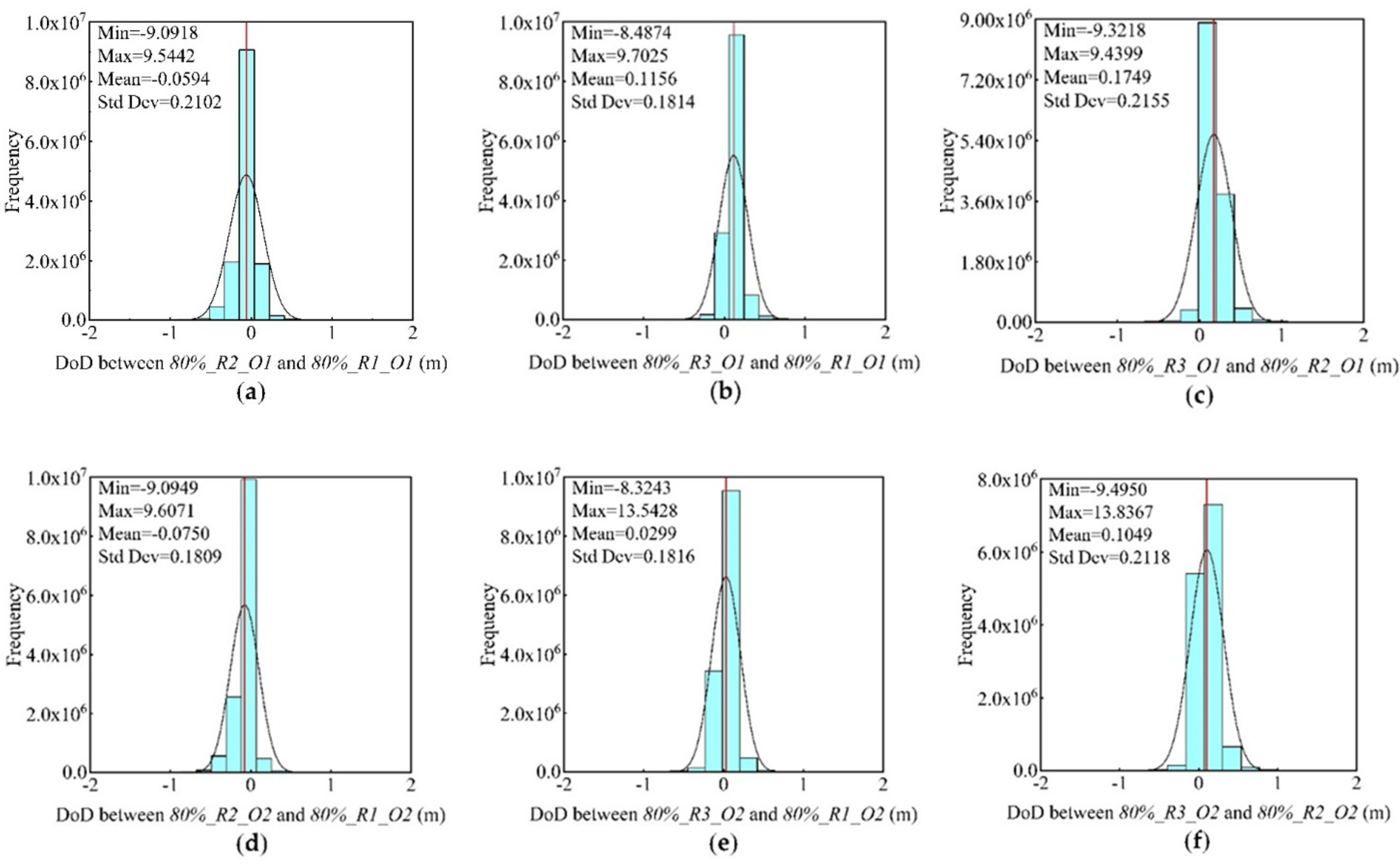
4.2. Internal Precision Analysis
4.3. External Precision Analysis
5. Discussion
6. Conclusions
Author Contributions
Funding
Institutional Review Board Statement
Informed Consent Statement
Data Availability Statement
Conflicts of Interest
References
- Li, D.R.; Li, M. Research advance and application prospect of unmanned aerial vehicle remote sensing system. Geomat. Inf. Sci. Wuhan Univ. 2014, 39, 505–513. [Google Scholar] [CrossRef]
- Yang, B.S.; Li, J.P. Implementation of a low-cost mini-UAV laser scanning system. Geomat. Inf. Sci. Wuhan Univ. 2018, 43, 1972–1978. [Google Scholar] [CrossRef]
- Michaelides, R.J.; Chen, R.H.; Zhao, Y.; Schaefer, K.; Parsekian, A.D.; Sullivan, T.; Moghaddam, M.; Zebker, H.A.; Liu, L.; Xu, X.; et al. Permafrost dynamics observatory-part I: Postprocessing and calibration methods of UAVSAR L-band InSAR data for seasonal subsidence rstimation. Earth Space Sci. 2021, 8, e2020EA001630. [Google Scholar] [CrossRef]
- Zhang, J.X.; Liu, F.; Wang, J. Review of the light-weighted and small UAV system for aerial photography and remote sensing. Natl. Remote Sens. Bull. 2021, 25, 708–724. [Google Scholar] [CrossRef]
- Li, X.; Xiong, B.S.; Yuan, Z.D.; He, K.F.; Liu, X.L.; Liu, Z.M.; Shen, Z.Q. Evaluating the potentiality of using control-free images from a mini Unmanned Aerial Vehicle (UAV) and Structure-from-Motion (SfM) photogrammetry to measure paleoseismic offsets. Int. J. Remote Sens. 2021, 42, 2417–2439. [Google Scholar] [CrossRef]
- Fernandez, T.; Perez, J.L.; Cardenal, J.; Gomez, J.M.; Colomo, C.; Delgado, J. Analysis of landslide evolution affecting Olive Groves using UAV and photogrammetric techniques. Remote Sens. 2016, 8, 29. [Google Scholar] [CrossRef] [Green Version]
- Anders, N.; Smith, M.; Suomalainen, J.; Cammeraat, E.; Valente, J.; Keesstra, S. Impact of flight altitude and cover orientation on Digital Surface Model (DSM) accuracy for flood damage assessment in Murcia (Spain) using a fixed-wing UAV. Earth Sci. Inform. 2020, 13, 391–404. [Google Scholar] [CrossRef] [Green Version]
- Dai, W.Q.; LI, H.; Gong, Z.; Zhang, C.K.; Zhou, Z. Application of unmanned aerial vehicle technology in geomorphological evolution of tidal flat. Adv. Water Sci. 2019, 30, 359–372. [Google Scholar] [CrossRef]
- Liu, Y.; Feng, H.K.; Huang, J.; Sun, Q.; Yang, F.Q.; Yang, G.J. Estimation of potato plant height and above-ground biomass based on UAV hyperspectral images. Trans. Chin. Soc. Agric. Mach. 2021, 52, 188–198. [Google Scholar] [CrossRef]
- Yang, Y.C.; Qi, Y.B.; Fu, J.X.; Wu, J. DEM based geomorphic features and classification: A case study in the Pisha sandstone area. Sci. Soil Water Conserv. 2019, 17, 1–10. [Google Scholar] [CrossRef]
- Garcia, G.P.B.; Grohmann, C.H. DEM-based geomorphological mapping and landforms characterization of a tropical karst environment in southeastern Brazil. J. S. Am. Earth Sci. 2019, 93, 14–22. [Google Scholar] [CrossRef] [Green Version]
- Lian, H.Q.; Meng, L.; Han, R.G.; Yang, Y.; Yu, B. Geological information extraction based on remote sensing of unmanned aerial vehicle: Exemplified by Liujiang Basin. Remote Sens. Land Resour. 2020, 32, 136–142. [Google Scholar] [CrossRef]
- Meinen, B.U.; Robinson, D.T. Mapping erosion and deposition in an agricultural landscape: Optimization of UAV image acquisition schemes for SfM-MVS. Remote Sens. Environ. 2020, 239, 10. [Google Scholar] [CrossRef]
- Hugenholtz, C.H.; Whitehead, K.; Brown, O.W.; Barchyn, T.E.; Moorman, B.J.; LeClair, A.; Riddell, K.; Hamilton, T. Geomorphological mapping with a small unmanned aircraft system (sUAS): Feature detection and accuracy assessment of a photogrammetrically-derived digital terrain model. Geomorphology 2013, 194, 16–24. [Google Scholar] [CrossRef] [Green Version]
- Elkhrachy, I. Accuracy assessment of low-cost Unmanned Aerial Vehicle (UAV) photogrammetry. Alex. Eng. J. 2021, 60, 5579–5590. [Google Scholar] [CrossRef]
- Liu, Y.S.; Qin, X.; Guo, W.Q.; Gao, S.R.; Chen, J.Z.; Wang, L.H.; Li, Y.X.; Jin, Z.Z. Influence of the use of photogrammetric measurement precision on low-altitude micro-UAVs in the glacier region. Natl. Remote Sens. Bull. 2020, 24, 161–172. [Google Scholar] [CrossRef]
- Zhu, J.; Ding, Y.Z.; Chen, P.J.; Wang, X.A.; Guo, B.X.; Xiao, X.W.; Niu, K.K. Influence of control points’ layout on aero-triangulation accuracy for UAV images. Sci. Surv. Mapp. 2016, 41, 116–120. [Google Scholar] [CrossRef]
- Sanz-Ablanedo, E.; Chandler, J.H.; Rodríguez-Pérez, J.R.; Ordóñez, C. Accuracy of Unmanned Aerial Vehicle (UAV) and SfM photogrammetry survey as a function of the number and location of ground control points used. Remote Sens. 2018, 10, 1606. [Google Scholar] [CrossRef] [Green Version]
- Li, Z.J.; Zhong, L.T.; Huang, Y.H.; Ge, H.L.; Zhu, Y.; Jiang, F.S.; Li, X.F.; Zhang, Y.; Lin, J.S. Monitoring technology for collapse erosion based on the nap of the object photograph of UAV. Trans. Chin. Soc. Agric. Eng. 2021, 37, 151–159. [Google Scholar] [CrossRef]
- Gong, C.G.; Lei, S.G.; Bian, Z.F.; Liu, Y.; Zhang, Z.; Cheng, W. Analysis of the development of an erosion gully in an open-pit coal mine dump during a Winter freeze-thaw cycle by using low-cost UAVs. Remote Sens. 2019, 11, 17. [Google Scholar] [CrossRef] [Green Version]
- Brunetta, R.; Duo, E.; Ciavola, P. Evaluating short-term tidal flat evolution through UAV surveys: A case study in the Po Delta (Italy). Remote Sens. 2021, 13, 31. [Google Scholar] [CrossRef]
- Zhang, B.G.; Zhao, J.; Ma, C.; Li, T.; Cheng, X.; Liu, L.B. UAV photogrammetric monitoring of Antarctic ice doline formation. J. Beijing Norm. Univ. (Nat. Sci.) 2019, 55, 19–24. [Google Scholar] [CrossRef]
- Yin, S.L.; Tan, Y.Y.; Zhang, L.; Feng, W.; Liu, S.Y.; Jin, J. 3D outcrop geological modeling based on UAV oblique photography data: A case study of Pingtouxiang section in Lüliang City, Shanxi Province. J. Palaeogeogr. (Chin. Ed.) 2018, 20, 909–924. [Google Scholar] [CrossRef]
- Peppa, M.V.; Hall, J.; Goodyear, J.; Mills, J.P. Photogrammetric assessment and comparison of DJI Phantom 4 Pro and Phantom 4 RTK small unmanned aircraft systems. Int. Arch. Photogramm. Remote Sens. Spat. Inf. Sci. 2019, XLII-2/W13, 503–509. [Google Scholar] [CrossRef] [Green Version]
- Xiao, S.Y. Positioning accuracy analysis of aerial triangulation of UAV images without ground control points. J. Chongqing Jiaotong Univ. (Nat. Sci.) 2021, 40, 117–123. [Google Scholar] [CrossRef]
- Benassi, F.; Dall’Asta, E.; Diotri, F.; Forlani, G.; di Cella, U.M.; Roncella, R.; Santise, M. Testing accuracy and repeatability of UAV blocks oriented with GNSS-supported aerial triangulation. Remote Sens. 2017, 9, 23. [Google Scholar] [CrossRef] [Green Version]
- Zhao, C.X.; Yang, W.; Wang, Y.J.; Ding, B.H.; Xu, X.C. Changes in surface elevation and velocity of Parlung No.4 glacier in southeastern Tibetan Plateau: Monitoring by UAV technology. J. Beijing Norm. Univ. (Nat. Sci.) 2020, 56, 557–565. [Google Scholar] [CrossRef]
- Casella, V.; Chiabrando, F.; Franzini, M.; Manzino, A.M. Accuracy assessment of a photogrammetric UAV block by using different software and adopting diverse processing strategies. In Proceedings of the 5th International Conference on Geographical Information Systems Theory, Applications and Management (GISTAM), Heraklion, Greece, 3–5 May 2019; pp. 77–87. [Google Scholar]
- Forlani, G.; Dall’Asta, E.; Diotri, F.; di Cella, U.M.; Roncella, R.; Santise, M. Quality assessment of DSMs produced from UAV flights georeferenced with on-board RTK positioning. Remote Sens. 2018, 10, 22. [Google Scholar] [CrossRef] [Green Version]
- Clapuyt, F.; Vanacker, V.; Van Oost, K. Reproducibility of UAV-based earth topography reconstructions based on Structure-from-Motion algorithms. Geomorphology 2016, 260, 4–15. [Google Scholar] [CrossRef]
- Lowe, D.G. Distinctive image features from scale-invariant keypoints. Int. J. Comput. Vis. 2004, 60, 91–110. [Google Scholar] [CrossRef]
- Wu, C.C. Towards linear-time incremental Structure from Motion. In Proceedings of the 2013 International Conference on 3D Vision—3DV 2013, Seattle, WA, USA, 29 June–1 July 2013; pp. 127–134. [Google Scholar]
- Snavely, N.; Seitz, S.M.; Szeliski, R. Modeling the world from Internet photo collections. Int. J. Comput. Vis. 2008, 80, 189–210. [Google Scholar] [CrossRef] [Green Version]
- Xiao, X.W.; Guo, B.X.; Li, D.R.; Li, L.H.; Yang, N.; Liu, J.C.; Zhang, P.; Peng, Z. Multi-View Stereo matching based on self-adaptive patch and image grouping for multiple unmanned aerial vehicle imagery. Remote Sens. 2016, 8, 30. [Google Scholar] [CrossRef] [Green Version]
- Brasington, J.; Langham, J.; Rumsby, B. Methodological sensitivity of morphometric estimates of coarse fluvial sediment transport. Geomorphology 2003, 53, 299–316. [Google Scholar] [CrossRef]
- Cook, K.L. An evaluation of the effectiveness of low-cost UAVs and structure from motion for geomorphic change detection. Geomorphology 2017, 278, 195–208. [Google Scholar] [CrossRef]
- Alfredsen, K.; Haas, C.; Tuhtan, J.A.; Zinke, P. Brief Communication: Mapping river ice using drones and structure from motion. Cryosphere 2018, 12, 627–633. [Google Scholar] [CrossRef] [Green Version]
- Pagan, J.I.; Banon, L.; Lopez, I.; Banon, C.; Aragones, L. Monitoring the dune-beach system of Guardamar del Segura (Spain) using UAV, SfM and GIS techniques. Sci. Total Environ. 2019, 687, 1034–1045. [Google Scholar] [CrossRef]
- Yang, D.D.; Qiu, H.J.; Hu, S.; Pei, Y.Q.; Wang, X.G.; Du, C.; Long, Y.Q.; Cao, M.M. Influence of successive landslides on topographic changes revealed by multitemporal high-resolution UAS-based DEM. Catena 2021, 202, 13. [Google Scholar] [CrossRef]
- Bi, R.; Gan, S.; Yuan, X.P.; LI, R.B.; Hu, L.; Gao, S. Research on UAV elevation route planning and modeling analysis for complex mountain landslides in Dongchuan. Bull. Surv. Mapp. 2021, 63–67. [Google Scholar] [CrossRef]


| UVA Specifications | Camera Specifications | |||
|---|---|---|---|---|
| Aircraft | DJI Phantom 4 RTK | Sensor | FC6310R | |
| Take-off weight | 1391 g | Sensor format | 1” (CMOS) 13.2 mm × 8.8 mm | |
| Max flight speed | 50 km/h (Positioning) 58 km/h (Attitude) | Focal length | 8.8 mm | |
| Max flight time | 30 min | 35 mm equiv. focal length | 24 mm | |
| Max take-off altitude | 6000 m | Image resolution | 5472 × 3648 | |
| Satellite positioning systems | Asia | GPS + BeiDou + Galileo | Field of View | 84° |
| Other area | GPS + GLONASS + Galileo | |||
| GNSS positioning accuracy | Horizontal | 1 cm + 1 ppm (RMS) | Pixel size | 2.41 µm |
| Vertical | 1.5 cm + 1 ppm (RMS) | |||
| UAV Flight Parameters | ||
|---|---|---|
| Type of Image | Orthophoto | Oblique Image |
| Survey date | July 2021 | |
| Flight altitude (m) | 200 m | |
| Ground Sampling Distance (GSD, cm/px) | 5.48 cm/px | |
| Image forward overlap (%) | 80% | |
| Image side overlap (%) | 80% | |
| Main route angle (°) | 68° | |
| Camera angle (°) | −90° | −45° |
| RTK status | Fixed | |
| Flight time (min, s) | 10 min | 35 s |
| Number of images captured | 119 | 8 |
| Dataset | Type of Image | Number of Images | Area (km2) | Number of Tie-Points | Mean Density of Tie-Points (pts/m2) |
|---|---|---|---|---|---|
| orthophoto | 119 | 0.0647 | 138,924 | 0.35 | |
| 0.0619 | 123,707 | 0.30 | |||
| 0.0648 | 136,996 | 0.35 | |||
| Oblique image | 127 (8 of oblique images) | 0.0660 | 144,410 | 0.36 | |
| 0.0671 | 128,634 | 0.30 | |||
| 0.0666 | 144,407 | 0.36 |
| Dataset | Error (m) | ||||
|---|---|---|---|---|---|
| 0.0265 | 0.0338 | 0.2832 | 0.0430 | 0.2865 | |
| 0.0232 | 0.0380 | 0.2554 | 0.0445 | 0.2593 | |
| 0.0311 | 0.0340 | 0.3761 | 0.0461 | 0.3789 | |
| 0.0269 | 0.0353 | 0.3049 | 0.0445 | 0.3082 | |
| 0.0240 | 0.0231 | 0.0968 | 0.0333 | 0.1024 | |
| 0.0191 | 0.0300 | 0.0683 | 0.0356 | 0.0770 | |
| 0.0182 | 0.0272 | 0.1175 | 0.0327 | 0.1220 | |
| 0.0204 | 0.0267 | 0.0942 | 0.0339 | 0.1005 | |
| Dataset 1 | Dataset 2 | Error (m) | ||||
|---|---|---|---|---|---|---|
| 0.0300 | 0.0289 | 0.0487 | 0.0416 | 0.0641 | ||
| 0.0281 | 0.0272 | 0.1058 | 0.0391 | 0.1128 | ||
| 0.0288 | 0.0290 | 0.1273 | 0.0409 | 0.1337 | ||
| 0.0290 | 0.0284 | 0.0939 | 0.0405 | 0.1035 | ||
| 0.0304 | 0.0301 | 0.0477 | 0.0427 | 0.0640 | ||
| 0.0240 | 0.0302 | 0.0521 | 0.0386 | 0.0648 | ||
| 0.0276 | 0.0339 | 0.0657 | 0.0437 | 0.0790 | ||
| 0.0273 | 0.0314 | 0.0552 | 0.0417 | 0.0693 | ||
| Dataset 1 | Dataset 2 | Error (m) | Std Dev | ||
|---|---|---|---|---|---|
| Minimum | Maximum | Mean | |||
| −9.0918 | 9.5442 | −0.0594 | 0.2102 | ||
| −8.4874 | 9.7025 | 0.1156 | 0.1814 | ||
| −9.3218 | 9.4399 | 0.1749 | 0.2155 | ||
| 8.9670 | 9.5622 | 0.1166 | 0.2024 | ||
| −9.0949 | 9.6071 | −0.0750 | 0.1809 | ||
| −8.3243 | 13.5428 | 0.0299 | 0.1816 | ||
| −9.4950 | 13.8367 | 0.1049 | 0.2118 | ||
| 8.9514 | 12.3289 | 0.0700 | 0.1914 | ||
| Dataset | Error (m) | ||||
|---|---|---|---|---|---|
| 0.0264 | 0.0244 | 0.1338 | 0.0360 | 0.1385 | |
| 0.0250 | 0.0225 | 0.1234 | 0.0336 | 0.1279 | |
| 0.0270 | 0.0223 | 0.1385 | 0.0350 | 0.1429 | |
| 0.0225 | 0.0205 | 0.1225 | 0.0305 | 0.1262 | |
| 0.0191 | 0.0300 | 0.0683 | 0.0356 | 0.0770 | |
| Dataset 1 | Dataset 2 | Error (m) | Std Dev | ||
|---|---|---|---|---|---|
| Minimum | Maximum | Mean | |||
| −8.6395 | 9.2965 | 0.0772 | 0.1493 | ||
| −9.6110 | 9.1234 | 0.0489 | 0.1518 | ||
| −9.5295 | 8.5393 | 0.0865 | 0.1244 | ||
| −9.6611 | 8.4387 | 0.0415 | 0.1208 | ||
| Dataset | ||
|---|---|---|
| 3707.94 | 3707.94 | |
| 3707.94 | ||
| 3707.94 | ||
| 3707.94 | 3708.14 | |
| 3708.23 | ||
| 3708.24 |
| Dataset | Mean Image Spacing (m) | Mean Image Overlap (%) |
|---|---|---|
| 268.6780 | 0 | |
| 39.2523 | 83.16 | |
| 78.8377 | 66.89 | |
| 39.4021 | 85.18 | |
| 38.3829 | 84.58 |
Publisher’s Note: MDPI stays neutral with regard to jurisdictional claims in published maps and institutional affiliations. |
© 2021 by the authors. Licensee MDPI, Basel, Switzerland. This article is an open access article distributed under the terms and conditions of the Creative Commons Attribution (CC BY) license (https://creativecommons.org/licenses/by/4.0/).
Share and Cite
Bi, R.; Gan, S.; Yuan, X.; Li, R.; Gao, S.; Luo, W.; Hu, L. Studies on Three-Dimensional (3D) Accuracy Optimization and Repeatability of UAV in Complex Pit-Rim Landforms As Assisted by Oblique Imaging and RTK Positioning. Sensors 2021, 21, 8109. https://doi.org/10.3390/s21238109
Bi R, Gan S, Yuan X, Li R, Gao S, Luo W, Hu L. Studies on Three-Dimensional (3D) Accuracy Optimization and Repeatability of UAV in Complex Pit-Rim Landforms As Assisted by Oblique Imaging and RTK Positioning. Sensors. 2021; 21(23):8109. https://doi.org/10.3390/s21238109
Chicago/Turabian StyleBi, Rui, Shu Gan, Xiping Yuan, Raobo Li, Sha Gao, Weidong Luo, and Lin Hu. 2021. "Studies on Three-Dimensional (3D) Accuracy Optimization and Repeatability of UAV in Complex Pit-Rim Landforms As Assisted by Oblique Imaging and RTK Positioning" Sensors 21, no. 23: 8109. https://doi.org/10.3390/s21238109
APA StyleBi, R., Gan, S., Yuan, X., Li, R., Gao, S., Luo, W., & Hu, L. (2021). Studies on Three-Dimensional (3D) Accuracy Optimization and Repeatability of UAV in Complex Pit-Rim Landforms As Assisted by Oblique Imaging and RTK Positioning. Sensors, 21(23), 8109. https://doi.org/10.3390/s21238109