
Detection of Collaterals from Cone-Beam CT Images in Stroke

 , , ,
, , ,
Abstract
:1. Introduction
2. Related Works
2.1. Artifact Removal
2.2. Vessel Enhancement
2.3. Feature Extraction
2.4. Classification
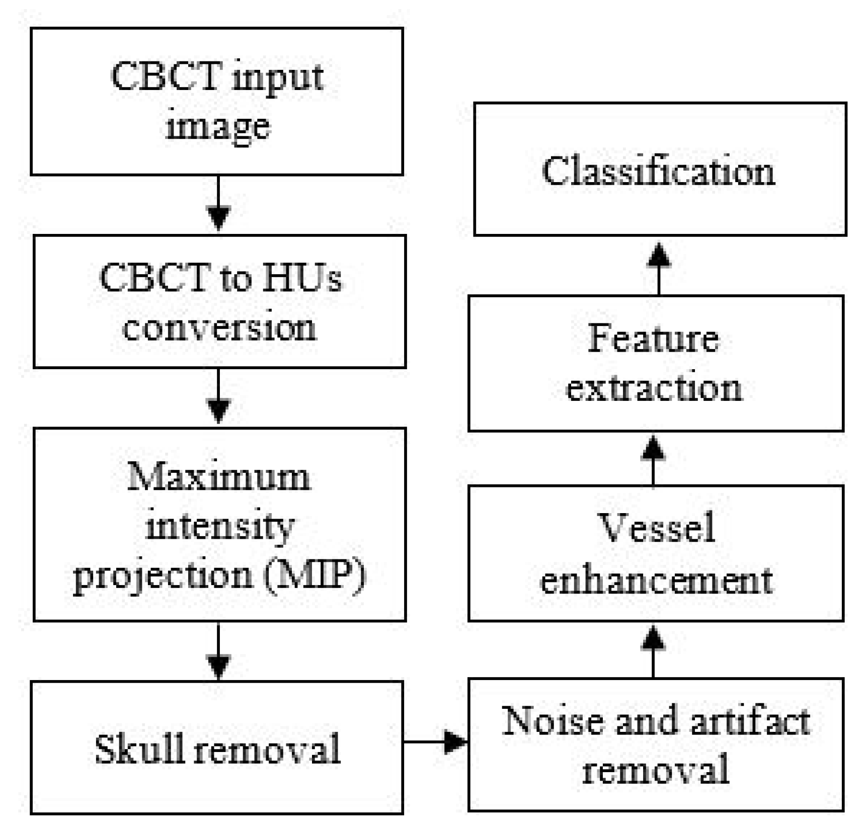
3. Methodology
3.1. Image Acquisition
3.2. Conversion of CBCT to CT Values
3.3. Maximum Intensity Projection
3.4. Skull Removal
3.5. Noise and Artifact Removal
3.6. Vessel Enhancement
3.7. Feature Extraction
3.8. Classification
3.9. Performance Measures
4. Results and Discussion
4.1. HU Conversion and MIP Projection
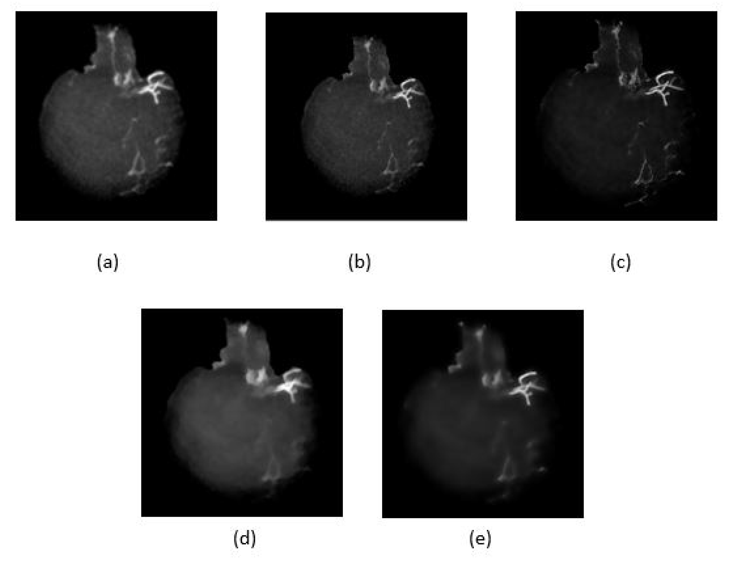
4.2. Artifact Removal
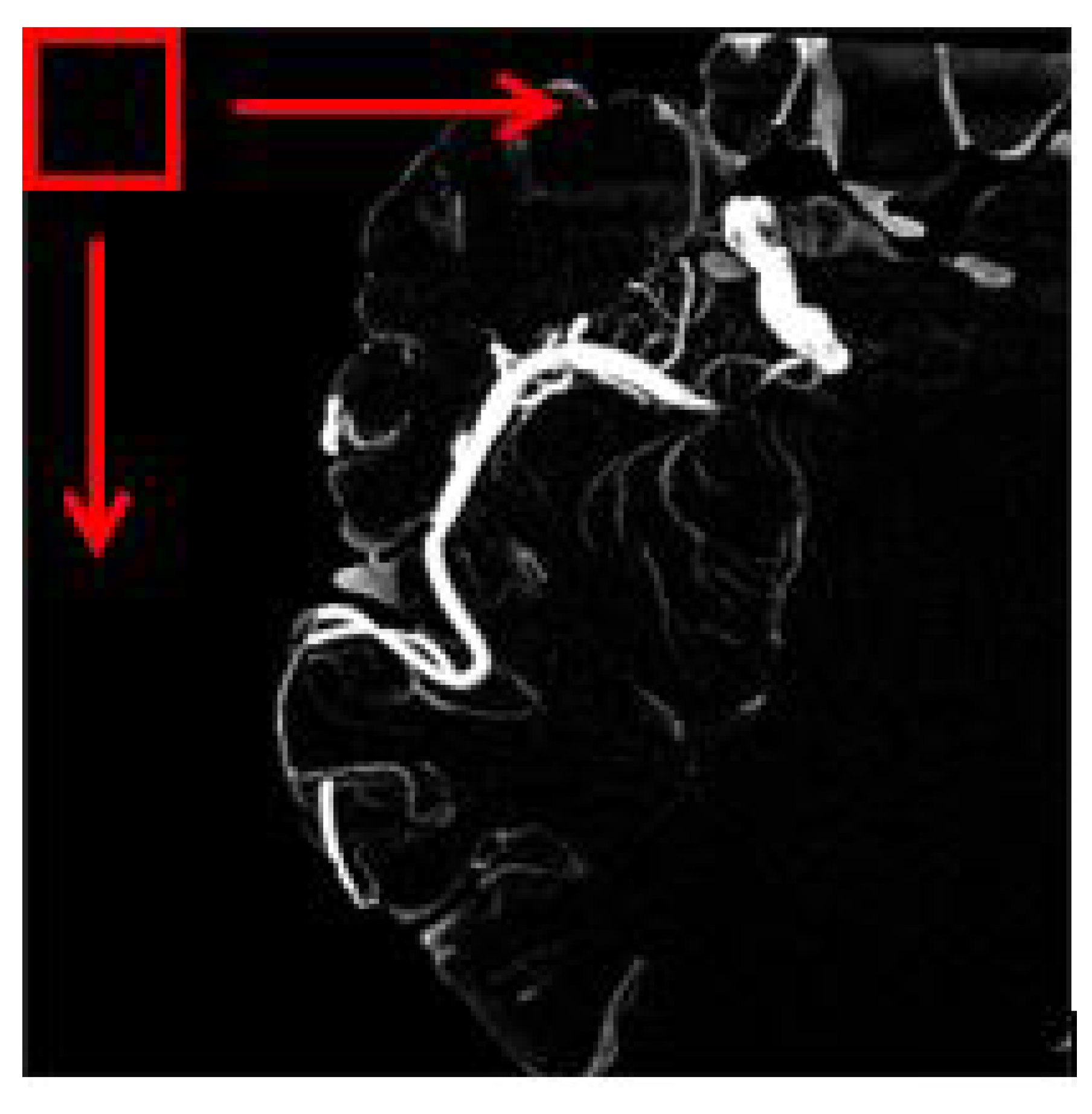
4.3. Vessel Enhancement
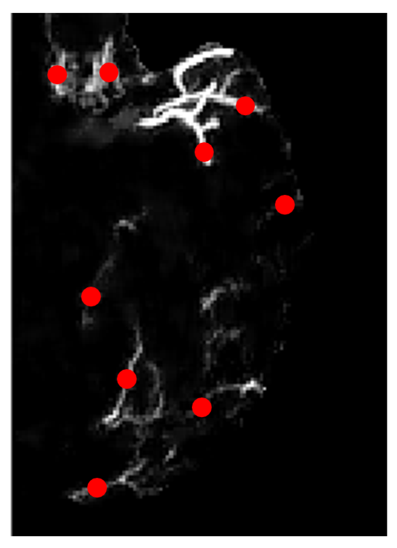
4.4. Feature Extraction
4.5. Performance of Classifiers
5. Conclusions
Author Contributions
Funding
Institutional Review Board Statement
Informed Consent Statement
Data Availability Statement
Acknowledgments
Conflicts of Interest
References
- Lee, Y.; Shafie, A.; Sidek, N.; Aziz, Z. Economic burden of stroke in malaysia: Results from national neurology registry. J. Neurol. Sci. 2017, 381, 167–168. [Google Scholar] [CrossRef]
- Galimanis, A.; Jung, S.; Mono, M.L.; Fischer, U.; Findling, O.; Weck, A.; Meier, N.; Marco De Marchis, G.; Brekenfeld, C.; El-Koussy, M.; et al. Endovascular therapy of 623 patients with anterior circulation stroke. Stroke 2012, 43, 1052–1057. [Google Scholar] [CrossRef] [PubMed] [Green Version]
- Kucinski, T.; Koch, C.; Eckert, B.; Becker, V.; Krömer, H.; Heesen, C.; Grzyska, U.; Freitag, H.; Röther, J.; Zeumer, H. Collateral circulation is an independent radiological predictor of outcome after thrombolysis in acute ischaemic stroke. Neuroradiology 2003, 45, 11–18. [Google Scholar] [CrossRef] [PubMed]
- Bang, O.Y.; Saver, J.L.; Kim, S.J.; Kim, G.M.; Chung, C.S.; Ovbiagele, B.; Lee, K.H.; Liebeskind, D.S. Collateral flow predicts response to endovascular therapy for acute ischemic stroke. Stroke 2011, 42, 693–699. [Google Scholar] [CrossRef] [PubMed] [Green Version]
- Bang, O.Y.; Saver, J.L.; Kim, S.J.; Kim, G.M.; Chung, C.S.; Ovbiagele, B.; Lee, K.H.; Liebeskind, D.S.; UCLA-Samsung Stroke Collaborators. Collateral flow averts hemorrhagic transformation after endovascular therapy for acute ischemic stroke. Stroke 2011, 42, 2235–2239. [Google Scholar] [CrossRef] [PubMed] [Green Version]
- Shuaib, A.; Butcher, K.; Mohammad, A.A.; Saqqur, M.; Liebeskind, D.S. Collateral blood vessels in acute ischaemic stroke: A potential therapeutic target. Lancet Neurol. 2011, 10, 909–921. [Google Scholar] [CrossRef]
- Ibraheem, I. Reduction of artifacts in dental cone beam CT images to improve the three dimensional image reconstruction. J. Biomed. Sci. Eng. 2012, 5, 409–415. [Google Scholar] [CrossRef] [Green Version]
- Scarfe, W.C.; Farman, A.G. What is cone-beam CT and how does it work? Dent. Clin. N. Am. 2008, 52, 707–730. [Google Scholar] [CrossRef]
- McKinley, R.; Häni, L.; Gralla, J.; El-Koussy, M.; Bauer, S.; Arnold, M.; Fischer, U.; Jung, S.; Mattmann, K.; Reyes, M.; et al. Fully automated stroke tissue estimation using random forest classifiers (FASTER). J. Cereb. Blood Flow Metab. 2017, 37, 2728–2741. [Google Scholar] [CrossRef] [Green Version]
- Chiaradia, M.; Radaelli, A.; Campeggi, A.; Bouanane, M.; De La Taille, A.; Kobeiter, H. Automatic three-dimensional detection of prostatic arteries using cone-beam CT during prostatic arterial embolization. J. Vasc. Interv. Radiol. 2015, 26, 413–417. [Google Scholar] [CrossRef]
- Schulze, R.; Heil, U.; Groβ, D.; Bruellmann, D.; Dranischnikow, E.; Schwanecke, U.; Schoemer, E. Artefacts in CBCT: A review. Dentomaxillofac. Radiol. 2011, 40, 265–273. [Google Scholar] [CrossRef] [Green Version]
- Iqbal, S. A comprehensive study of the anatomical variations of the circle of willis in adult human brains. J. Clin. Diagn. Res. JCDR 2013, 7, 2423. [Google Scholar] [CrossRef] [PubMed]
- Akbari, H.; Kosugi, Y.; Kojima, K.; Tanaka, N. Blood vessel detection and artery-vein differentiation using hyperspectral imaging. In Proceedings of the 2009 Annual International Conference of the IEEE Engineering in Medicine and Biology Society, Minneapolis, MN, USA, 3–6 September 2009; pp. 1461–1464. [Google Scholar] [CrossRef]
- Preethi, M.; Vanithamani, R. Review of retinal blood vessel detection methods for automated diagnosis of Diabetic Retinopathy. In Proceedings of the IEE International Conference on Advances In Engineering, Science And Management (ICAESM-2012), Nagapattinam, India, 30–31 March 2012; pp. 262–265. [Google Scholar]
- Thakur, A.; Malik, M.; Phutela, N.; Khare, P.; Mor, P. CBCT image noise reduction and enhancement using Bi-Histogram method with bent activation function. In Proceedings of the International Conference on Information Technology (InCITe)—The Next Generation IT Summit on the Theme-Internet of Things: Connect your Worlds, Noida, India, 6–7 October 2016; pp. 242–246. [Google Scholar]
- Liang, X.; Zhang, Z.; Niu, T.; Yu, S.; Wu, S.; Li, Z.; Zhang, H.; Xie, Y. Iterative image-domain ring artifact removal in cone-beam CT. Phys. Med. Biol. 2017, 62, 5276. [Google Scholar] [CrossRef] [PubMed]
- Yilmaz, E.; Kayikcioglu, T.; Kayipmaz, S. Noise removal of CBCT images using an adaptive anisotropic diffusion filter. In Proceedings of the 40th International Conference on Telecommunications and Signal Processing (TSP), Barcelona, Spain, 5–7 July 2017; pp. 650–653. [Google Scholar]
- Zhang, Y.; Zhang, L.; Zhu, X.R.; Lee, A.K.; Chambers, M.; Dong, L. Reducing metal artifacts in cone-beam CT images by preprocessing projection data. Int. J. Radiat. Oncol. Biol. Phys. 2007, 67, 924–932. [Google Scholar] [CrossRef]
- Chen, Y.W.; Duan, G.; Fujita, A.; Hirooka, K.; Ueno, Y. Ring artifacts reduction in cone-beam CT images based on independent component analysis. In Proceedings of the Conference on Instrumentation and Measurement Technology, Singapore, 5–7 May 2009; pp. 1734–1737. [Google Scholar]
- Altunbas, C.; Lai, C.J.; Zhong, Y.; Shaw, C.C. Reduction of ring artifacts in CBCT: Detection and correction of pixel gain variations in flat panel detectors. Med. Phys. 2014, 41, 091913. [Google Scholar] [CrossRef]
- Yılmaz, E.; Kayıkçıoğlu, T.; Kayıpmaz, S. Experimental comparison of different noise reduction techniques on cone beam computed tomography images. In Proceedings of the 22nd Conference on Signal Processing and Communications Applications (SIU), Trabzon, Turkey, 23–25 April 2014; pp. 2086–2089. [Google Scholar]
- Perona, P.; Malik, J. Scale-space and edge detection using anisotropic diffusion. IEEE Trans. Pattern Anal. Mach. Intell. 1990, 12, 629–639. [Google Scholar] [CrossRef] [Green Version]
- Crete, F.; Dolmiere, T.; Ladret, P.; Nicolas, M. The blur effect: Perception and estimation with a new no-reference perceptual blur metric. In Human Vision and Electronic Imaging XII; International Society for Optics and Photonics: Bellingham, WA, USA, 2007; Volume 6492, p. 64920I. [Google Scholar]
- Huo, Q.; Li, J.; Lu, Y.; Yan, Z. Removing ring artifacts in CBCT images via smoothing. Int. J. Imaging Syst. Technol. 2016, 26, 284–294. [Google Scholar] [CrossRef]
- Xu, L.; Yan, Q.; Xia, Y.; Jia, J. Structure extraction from texture via relative total variation. ACM Trans. Graph. TOG 2012, 31, 1–10. [Google Scholar] [CrossRef]
- Chen, W.; Prell, D.; Kalender, W. Accelerating ring artifact correction for flat-detector CT using the CUDA framework. In Medical Imaging 2010: Physics of Medical Imaging; International Society for Optics and Photonics: Bellingham, WA, USA, 2010; Volume 7622, p. 76223A. [Google Scholar]
- Wei, Z.; Wiebe, S.; Chapman, D. Ring artifacts removal from synchrotron CT image slices. J. Instrum. 2013, 8, C06006. [Google Scholar] [CrossRef]
- Dufour, A.; Tankyevych, O.; Naegel, B.; Talbot, H.; Ronse, C.; Baruthio, J.; Dokládal, P.; Passat, N. Filtering and segmentation of 3D angiographic data: Advances based on mathematical morphology. Med. Image Anal. 2013, 17, 147–164. [Google Scholar] [CrossRef] [PubMed] [Green Version]
- Truc, P.T.; Khan, M.A.; Lee, Y.K.; Lee, S.; Kim, T.S. Vessel enhancement filter using directional filter bank. Comput. Vis. Image Underst. 2009, 113, 101–112. [Google Scholar] [CrossRef]
- Hsu, C.Y.; Schneller, B.; Ghaffari, M.; Alaraj, A.; Linninger, A. Medical image processing for fully integrated subject specific whole brain mesh generation. Technologies 2015, 3, 126–141. [Google Scholar] [CrossRef] [Green Version]
- Frangi, A.F.; Niessen, W.J.; Vincken, K.L.; Viergever, M.A. Multiscale vessel enhancement filtering. In Proceedings of the International Conference on Medical Image Computing and Computer-Assisted Intervention, Cambridge, MA, USA, 11–13 October 1998; Springer: Berlin/Heidelberg, Germany, 1998; pp. 130–137. [Google Scholar]
- Alharbi, S.S.; Sazak, Ç.; Nelson, C.J.; Obara, B. Curvilinear structure enhancement by multiscale top-hat tensor in 2D/3D images. In Proceedings of the International Conference on Bioinformatics and Biomedicine (BIBM), Madrid, Spain, 3–6 December 2018; pp. 814–822. [Google Scholar]
- Sun, K.; Chen, Z.; Jiang, S.; Wang, Y. Morphological multiscale enhancement, fuzzy filter and watershed for vascular tree extraction in angiogram. J. Med. Syst. 2011, 35, 811–824. [Google Scholar] [CrossRef]
- Bai, X.; Zhou, F. Analysis of new top-hat transformation and the application for infrared dim small target detection. Pattern Recognit. 2010, 43, 2145–2156. [Google Scholar] [CrossRef]
- Medjahed, S.A. A comparative study of feature extraction methods in images classification. Int. J. Image Graph. Signal Process. 2015, 7, 16. [Google Scholar] [CrossRef] [Green Version]
- Mishra, S.; Panda, M. Medical image retrieval using self-organising map on texture features. Future Comput. Inform. J. 2018, 3, 359–370. [Google Scholar] [CrossRef]
- Takala, V.; Ahonen, T.; Pietikäinen, M. Block-based methods for image retrieval using local binary patterns. In Proceedings of the Scandinavian Conference on Image Analysis, Joensuu, Finland, 19–22 June 2005; Springer: Berlin/Heidelberg, Germany, 2005; pp. 882–891. [Google Scholar]
- Reed, T.R.; Dubuf, J.H. A review of recent texture segmentation and feature extraction techniques. CVGIP Image Underst. 1993, 57, 359–372. [Google Scholar] [CrossRef]
- Haralick, R.M.; Shanmugam, K.; Dinstein, I.H. Textural features for image classification. IEEE Trans. Syst. Man Cybern. 1973, SMC-3, 610–621. [Google Scholar] [CrossRef] [Green Version]
- Soh, L.K.; Tsatsoulis, C. Texture analysis of SAR sea ice imagery using gray level co-occurrence matrices. IEEE Trans. Geosci. Remote Sens. 1999, 37, 780–795. [Google Scholar] [CrossRef] [Green Version]
- Ojala, T.; Pietikainen, M.; Maenpaa, T. Multiresolution gray-scale and rotation invariant texture classification with local binary patterns. IEEE Trans. Pattern Anal. Mach. Intell. 2002, 24, 971–987. [Google Scholar] [CrossRef]
- Dornaika, F.; Moujahid, A.; El Merabet, Y.; Ruichek, Y. A comparative study of image segmentation algorithms and descriptors for building detection. In Handbook of Neural Computation; Elsevier: Amsterdam, The Netherlands, 2017; pp. 591–606. [Google Scholar]
- Gunay, A.; Nabiyev, V.V. Automatic age classification with LBP. In Proceedings of the 23rd International Symposium on Computer and Information Sciences, Istanbul, Turkey, 27–29 October 2008; pp. 1–4. [Google Scholar]
- Alhindi, T.J.; Kalra, S.; Ng, K.H.; Afrin, A.; Tizhoosh, H.R. Comparing LBP, HOG and deep features for classification of histopathology images. In Proceedings of the International Joint Conference on Neural Networks (IJCNN), Rio de Janeiro, Brazil, 8–13 July 2018; pp. 1–7. [Google Scholar]
- Clausi, D.A. An analysis of co-occurrence texture statistics as a function of grey level quantization. Can. J. Remote Sens. 2002, 28, 45–62. [Google Scholar] [CrossRef]
- Mingqiang, Y.; Kidiyo, K.; Joseph, R. A survey of shape feature extraction techniques. Pattern Recognit. 2008, 15, 43–90. [Google Scholar]
- Ranjidha, A.; Ramesh Kumar, A.; Saranya, M. Survey on medical image retrieval based on shape features and relevance vector machine classification. Int. J. Emerg. Trends Technol. Comput. Sci. IJETTCS 2013, 2, 333–339. [Google Scholar]
- Chaugule, A.; Mali, S.N. Evaluation of texture and shape features for classification of four paddy varieties. J. Eng. 2014, 2014. [Google Scholar] [CrossRef] [Green Version]
- Hu, M.K. Visual pattern recognition by moment invariants. IRE Trans. Inf. Theory 1962, 8, 179–187. [Google Scholar]
- Nixon, M.; Aguado, A. Feature Extraction and Image Processing for Computer Vision; Academic Press: Cambridge, MA, USA, 2019. [Google Scholar]
- Jain, A. Fundamentals of Digital Image Processing; Prentice Hall of India Private Limited: Upper Saddle River, NJ, USA, 1995. [Google Scholar]
- Steven, L.E.; Rafael, C.G.; Richard, E.W. Digital Image Processing Using Matlab; Princeton Hall Pearson Education: Upper Saddle River, NJ, USA, 2004. [Google Scholar]
- Altman, N.S. An introduction to kernel and nearest-neighbor nonparametric regression. Am. Stat. 1992, 46, 175–185. [Google Scholar]
- Cortes, C.; Vapnik, V. Support-vector networks. Mach. Learn. 1995, 20, 273–297. [Google Scholar] [CrossRef]
- Amelio, L.; Amelio, A. Classification methods in image analysis with a special focus on medical analytics. In Machine Learning Paradigms; Springer: Berlin/Heidelberg, Germany, 2019; pp. 31–69. [Google Scholar]
- Nardelli, P.; Jimenez-Carretero, D.; Bermejo-Pelaez, D.; Washko, G.R.; Rahaghi, F.N.; Ledesma-Carbayo, M.J.; San José Estépar, R. Pulmonary Artery–Vein Classification in CT Images Using Deep Learning. IEEE Trans. Med. Imaging 2018, 37, 2428–2440. [Google Scholar] [CrossRef]
- Girard, F.; Cheriet, F. Artery/vein classification in fundus images using CNN and likelihood score propagation. In Proceedings of the 2017 IEEE Global Conference on Signal and Information Processing (GlobalSIP), Montreal, QC, Canada, 14–16 November 2017; pp. 720–724. [Google Scholar] [CrossRef]
- Montagne, C.; Kodewitz, A.; Vigneron, V.; Giraud, V.; Lelandais, S. 3D Local Binary Pattern for PET image classification by SVM, Application to early Alzheimer disease diagnosis. In Proceedings of the 6th International Conference on Bio-Inspired Systems and Signal Processing (BIOSIGNALS 2013), Barcelona, Spain, 11–14 February 2013; pp. 145–150. [Google Scholar]
- Xiao, Z.; Ding, Y.; Lan, T.; Zhang, C.; Luo, C.; Qin, Z. Brain MR image classification for Alzheimer’s disease diagnosis based on multifeature fusion. Comput. Math. Methods Med. 2017, 2017, 1952373. [Google Scholar] [CrossRef] [PubMed]
- Yang, F.; Hamit, M.; Yan, C.B.; Yao, J.; Kutluk, A.; Kong, X.M.; Zhang, S.X. Feature extraction and classification on esophageal X-ray images of Xinjiang Kazak nationality. J. Healthc. Eng. 2017, 2017. [Google Scholar] [CrossRef] [PubMed] [Green Version]
- Hua, Y.; Nackaerts, O.; Duyck, J.; Maes, F.; Jacobs, R. Bone quality assessment based on cone beam computed tomography imaging. Clin. Oral Implant. Res. 2009, 20, 767–771. [Google Scholar] [CrossRef] [PubMed]
- Mah, P.; Reeves, T.; McDavid, W. Deriving Hounsfield units using grey levels in cone beam computed tomography. Dentomaxillofac. Radiol. 2010, 39, 323–335. [Google Scholar] [CrossRef] [PubMed]
- Chindasombatjaroen, J.; Kakimoto, N.; Shimamoto, H.; Murakami, S.; Furukawa, S. Correlation between pixel values in a cone-beam computed tomographic scanner and the computed tomographic values in a multidetector row computed tomographic scanner. J. Comput. Assist. Tomogr. 2011, 35, 662–665. [Google Scholar] [CrossRef] [PubMed]
- Zohra, F.T.; Gavrilov, A.D.; Duran, O.Z.; Gavrilova, M. A linear regression model for estimating facial image quality. In Proceedings of the 16th International Conference on Cognitive Informatics & Cognitive Computing (ICCI*CC), Oxford, UK, 26–28 July 2017; pp. 130–138. [Google Scholar]
- Sharma, K.; Soni, H.; Agarwal, K. Lung Cancer Detection in CT Scans of Patients Using Image Processing and Machine Learning Technique. In Advanced Computational and Communication Paradigms; Springer: Berlin/Heidelberg, Germany, 2018; pp. 336–344. [Google Scholar]
- García-Martinez, C.; Rodriguez, F.J.; Lozano, M. Analysing the significance of no free lunch theorems on the set of real-world binary problems. In Proceedings of the 11th International Conference on Intelligent Systems Design and Applications, Cordoba, Spain, 22–24 November 2011; pp. 344–349. [Google Scholar] [CrossRef]


| Features | Name | Methods |
|---|---|---|
| Texture | GLCM | Haralick Texture Feature [39], Soh et al. [40], and Clausi et al. [45] |
| Shape | SHAPE | Shape factors using region properties [48] |
| MOMENT | The seven Hu moment invariants [52] |
| Method | PSNR | SSIM |
|---|---|---|
| Anisotropic diffusion filter | 81.6645 | 0.9113 |
| Median filter | 82.7276 | 0.9112 |
| Wiener filter | 72.1510 | 0.9133 |
| L-RTV | 78.0170 | 0.8603 |
| L-RTV | 79.1176 | 0.8714 |
| Feature | Model | Accuracy (%) | Sensitivity (%) | Specificity (%) | Precision (%) | F-Measure (%) | AUC |
|---|---|---|---|---|---|---|---|
| GLCM | DET | 99.89 | 99.87 | 99.92 | 99.92 | 99.89 | 0.9990 |
| SVM | 99.92 | 99.87 | 99.98 | 99.98 | 99.93 | 0.9999 | |
| Random Forest | 99.85 | 99.96 | 99.75 | 99.75 | 99.85 | 0.9986 | |
| KNN | 97.41 | 98.46 | 96.40 | 96.31 | 97.37 | 0.9743 | |
| MOMENT INVARIANT | DET | 77.67 | 79.01 | 76.70 | 75.67 | 77.19 | 0.7785 |
| SVM | 77.58 | 69.21 | 99.33 | 99.58 | 81.64 | 0.8427 | |
| Random Forest | 78.04 | 69.83 | 98.07 | 98.75 | 81.81 | 0.8395 | |
| KNN | 68.33 | 75.65 | 64.37 | 54 | 62.89 | 0.7001 | |
| SHAPE | DET | 71.5 | 72.16 | 71.12 | 70.16 | 71.03 | 0.7164 |
| SVM | 72.20 | 71.07 | 74.02 | 75.91 | 73.23 | 0.7254 | |
| Random Forest | 78.41 | 76.18 | 81.63 | 83.75 | 79.64 | 0.7890 | |
| KNN | 79.33 | 77.14 | 82.14 | 83.66 | 80.21 | 0.7964 |
Publisher’s Note: MDPI stays neutral with regard to jurisdictional claims in published maps and institutional affiliations. |
© 2021 by the authors. Licensee MDPI, Basel, Switzerland. This article is an open access article distributed under the terms and conditions of the Creative Commons Attribution (CC BY) license (https://creativecommons.org/licenses/by/4.0/).
Share and Cite
Abd Aziz, A.; Izhar, L.I.; Asirvadam, V.S.; Tang, T.B.; Ajam, A.; Omar, Z.; Muda, S. Detection of Collaterals from Cone-Beam CT Images in Stroke. Sensors 2021, 21, 8099. https://doi.org/10.3390/s21238099
Abd Aziz A, Izhar LI, Asirvadam VS, Tang TB, Ajam A, Omar Z, Muda S. Detection of Collaterals from Cone-Beam CT Images in Stroke. Sensors. 2021; 21(23):8099. https://doi.org/10.3390/s21238099
Chicago/Turabian StyleAbd Aziz, Azrina, Lila Iznita Izhar, Vijanth Sagayan Asirvadam, Tong Boon Tang, Azimah Ajam, Zaid Omar, and Sobri Muda. 2021. "Detection of Collaterals from Cone-Beam CT Images in Stroke" Sensors 21, no. 23: 8099. https://doi.org/10.3390/s21238099
APA StyleAbd Aziz, A., Izhar, L. I., Asirvadam, V. S., Tang, T. B., Ajam, A., Omar, Z., & Muda, S. (2021). Detection of Collaterals from Cone-Beam CT Images in Stroke. Sensors, 21(23), 8099. https://doi.org/10.3390/s21238099