Figure 1.
Examples of concrete wearable devices, along with their typical on-body location, can be found in body area networks dedicated to patient monitoring. Both vital signs and body movements can be captured by these kinds of devices.
Figure 1.
Examples of concrete wearable devices, along with their typical on-body location, can be found in body area networks dedicated to patient monitoring. Both vital signs and body movements can be captured by these kinds of devices.
Figure 2.
Activity recognition chain defined in [
16] which includes the following (from
left to
right): data acquisition, signal preprocessing, segmentation, feature extraction, classification, and evaluation stages. From [
30].
Figure 2.
Activity recognition chain defined in [
16] which includes the following (from
left to
right): data acquisition, signal preprocessing, segmentation, feature extraction, classification, and evaluation stages. From [
30].
Figure 3.
Schematic of the typical units that compose a sensor (from left to right): transducer, amplifier, analog-to-digital converter (ADC), ADC postcorrection, and digital signal processing (DSP) units. The measurement of a phenomenon (measurand) as simple as temperature by a sensor is in and of itself an inductive process involving many biases. The action of the physico-electrical process of the sensor (via the units it encompasses) generates an electrical signal proportional to the physical phenomenon being measured. We, actually, do not have access to the physical phenomenon itself but to a representation provided through a transfer function deduced mathematically and that is specific to the physico-electrical process of the sensor. The choice of this process constitutes a bias similar to the elaboration of the transfer function.
Figure 6.
Various locations of wearable devices on the body. Illustration of a subject wearing the wearable sensors on the ear, chest, arm, wrist, waist, knee, and ankle.
Figure 6.
Various locations of wearable devices on the body. Illustration of a subject wearing the wearable sensors on the ear, chest, arm, wrist, waist, knee, and ankle.
Figure 7.
Framework of the proposed approach.
Figure 7.
Framework of the proposed approach.
Figure 8.
Basic learning setting where the learner is supplied with a fixed set of inductive biases. The inductive biases guide the learner in searching for the hypothesis that explain best the set of learning examples.
Figure 8.
Basic learning setting where the learner is supplied with a fixed set of inductive biases. The inductive biases guide the learner in searching for the hypothesis that explain best the set of learning examples.
Figure 9.
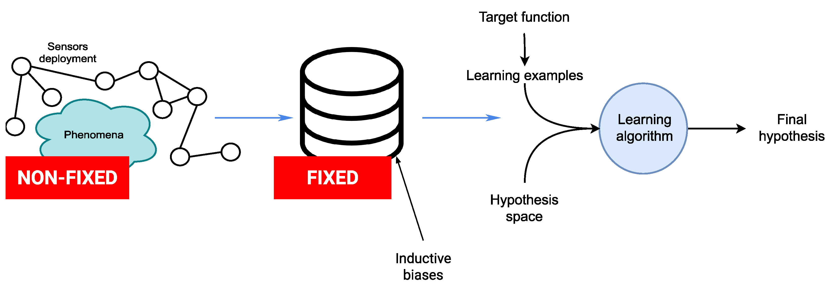
(left) Sensor-rich environment depicting a deployment of sensors surrounding a phenomena of interest. (center) Data repository where the fixed nature of the inductive biases used during the data generation process is highlighted. (right) The different components of the traditional learning processes. Learning processes in the case of sensor-rich environments deal very often with evolving and non-fixed settings materialized by the sensor deployments as well as the phenomenon of interest. This contrasts with the traditional setting where inductive biases are fixed beforehand and assumed to remain relevant during the entire deployment.
Figure 9.
(left) Sensor-rich environment depicting a deployment of sensors surrounding a phenomena of interest. (center) Data repository where the fixed nature of the inductive biases used during the data generation process is highlighted. (right) The different components of the traditional learning processes. Learning processes in the case of sensor-rich environments deal very often with evolving and non-fixed settings materialized by the sensor deployments as well as the phenomenon of interest. This contrasts with the traditional setting where inductive biases are fixed beforehand and assumed to remain relevant during the entire deployment.
Figure 10.
In the proposed framework, we are no longer required to fix the inductive biases beforehand as in the case of the traditional setting. The models describing both the deployment of sensors (in red) and the monitored phenomena itself (in green) serve to guide the learning process by providing the adequate inductive biases dynamically. More formally, the distribution Q can control the various scenarios that the activity recognition model will likely encounter in real-life deployment settings, such as the evolution of the deployment topology, the sensing platform, etc. As illustrated, the distribution Q can also control the evolution of the monitored phenomena.
Figure 11.
Global framework for uncertainty quantification [
91]. This framework is used to model the distribution
Q controlling the various scenarios that the activity recognition model will likely encounter in real-life deployment settings.
Figure 11.
Global framework for uncertainty quantification [
91]. This framework is used to model the distribution
Q controlling the various scenarios that the activity recognition model will likely encounter in real-life deployment settings.
Figure 12.
Architectural components used to construct the neural architectures. (a) Feature extraction (FE), (b) feature fusion (FF), (c) decision fusion (DF), and (d) analysis unit (AU).
Figure 12.
Architectural components used to construct the neural architectures. (a) Feature extraction (FE), (b) feature fusion (FF), (c) decision fusion (DF), and (d) analysis unit (AU).
Figure 13.
An example of architecture constructed using the architectural components depicted in
Figure 12. The nodes
and
correspond to the data sources.
Figure 13.
An example of architecture constructed using the architectural components depicted in
Figure 12. The nodes
and
correspond to the data sources.
Figure 14.
Highlighted in red is one of the paths that have as source node the data source denoted by and that is processed by the architectural components , , , and before joining the architecture’s output node.
Figure 14.
Highlighted in red is one of the paths that have as source node the data source denoted by and that is processed by the architectural components , , , and before joining the architecture’s output node.
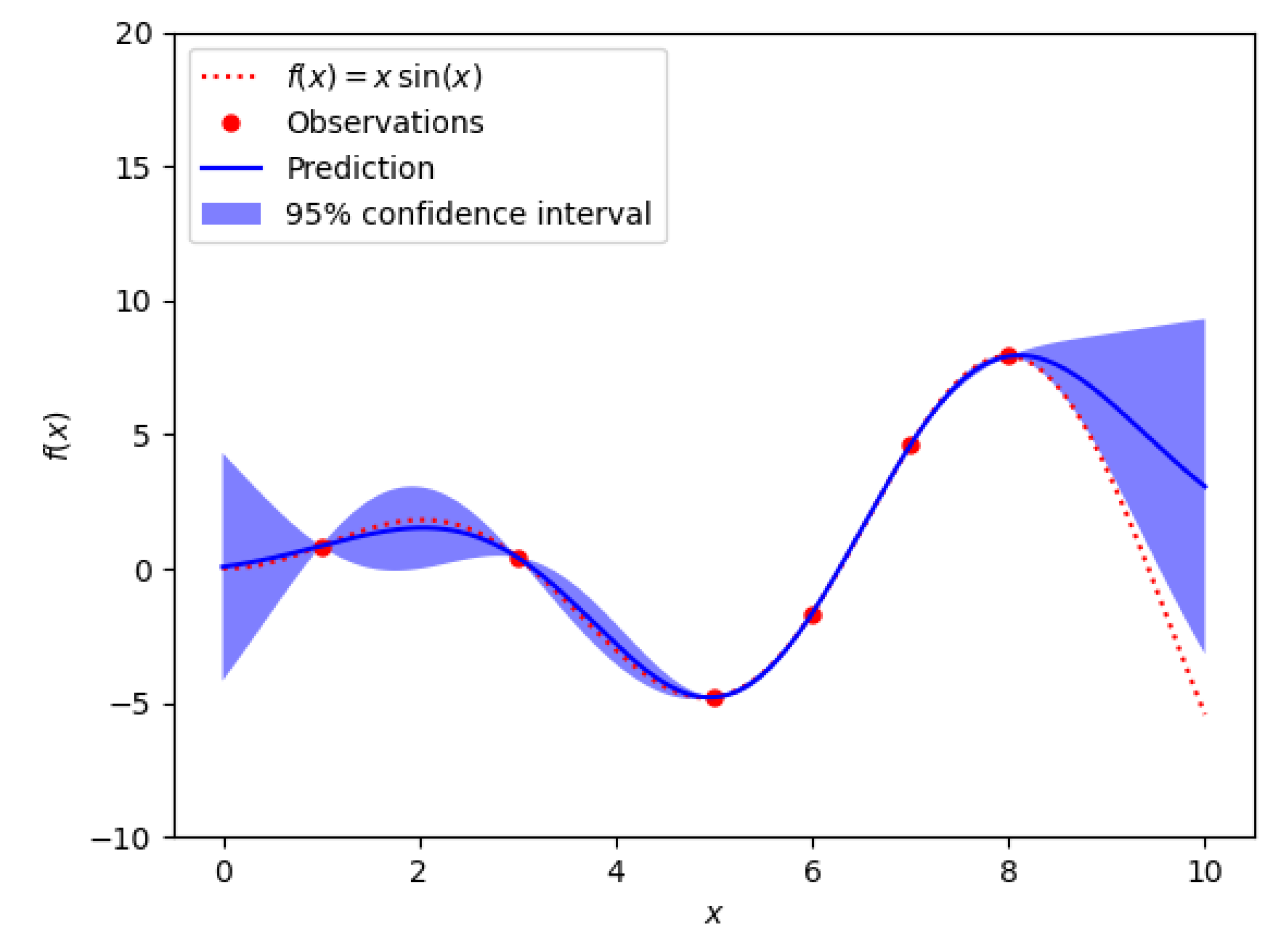
Figure 15.
An example of a Kriging (also known as Gaussian process modeling) metamodel The observations correspond to the actual evaluations of the hyperparameter instantiations. Kriging assumes that the true model is a trajectory of an underlying Gaussian process. The x-axis represents the design space (experimental points or realizations) while the y-axis represents the model’s response.
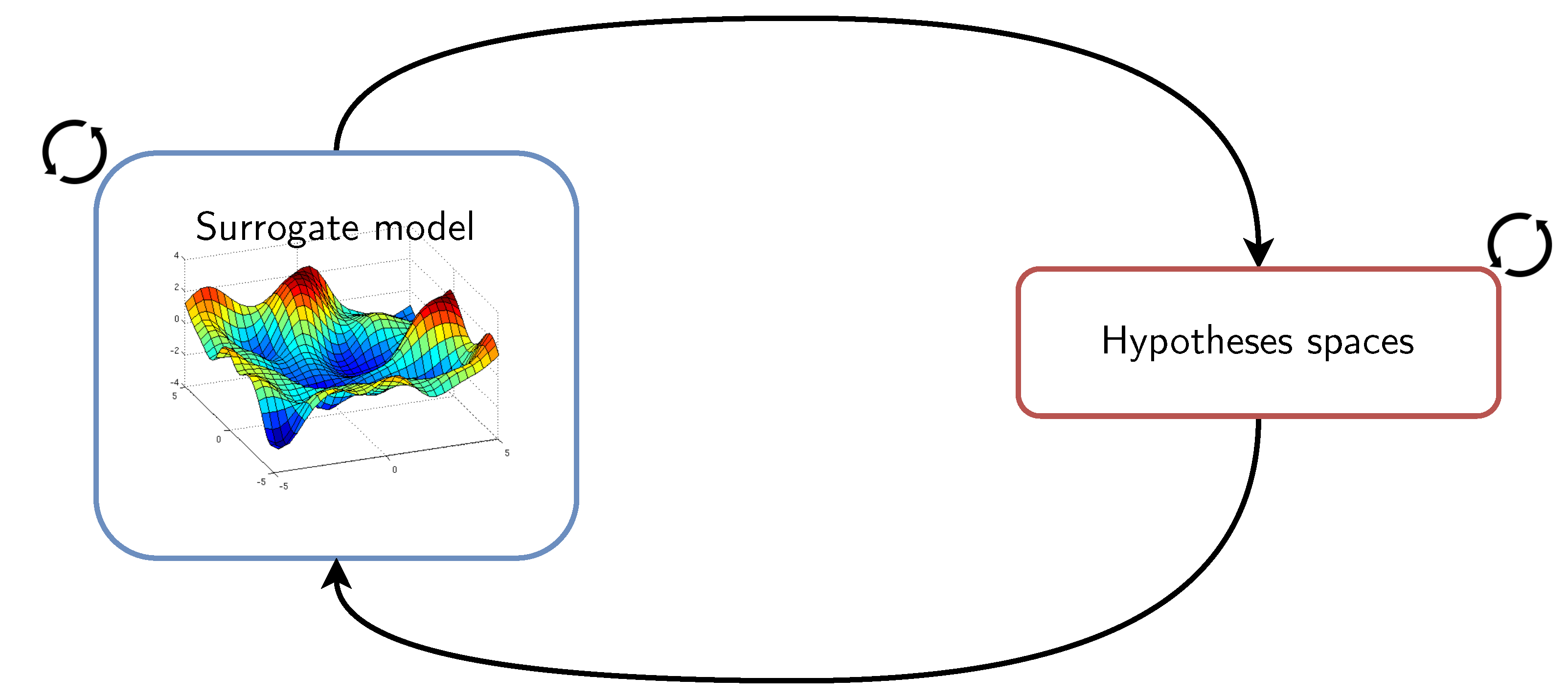
Figure 16.
Surrogate model-informed selection of inductive biases where, among the hypothesis spaces family , a set of concurrent hypothesis spaces (each of which containing a possibly suitable optimal hypothesis) is maintained throughout the learning process and model deployment.
Figure 16.
Surrogate model-informed selection of inductive biases where, among the hypothesis spaces family , a set of concurrent hypothesis spaces (each of which containing a possibly suitable optimal hypothesis) is maintained throughout the learning process and model deployment.
Figure 17.
Topology of the on-body sensors deployment featured by the SHL dataset, which is used in the experimental part of this paper. Data collection was performed by each participant using four smartphones simultaneously placed in different body locations: Hand, Torso, Hips, and Bag.
Figure 17.
Topology of the on-body sensors deployment featured by the SHL dataset, which is used in the experimental part of this paper. Data collection was performed by each participant using four smartphones simultaneously placed in different body locations: Hand, Torso, Hips, and Bag.
Figure 18.
Confusion matrix of the best model trained on all body locations fused together yielding 70.86% recognition performance measured by the f1-score. Best model among the set of models evaluated as part of a Bayesian optimization process involving the hyperparameters of the activity recognition chain.
Figure 19.
Pairwise marginal plots produced via the fANOVA framework [
115]. These plots illustrate the interplay (or the mutual impact influence) between some of the hyperparameters being optimized in (
a) interplay between kernel sizes 2 (
) and (
) (
b) interplay between the number of units of the dense layer (
) and kernel size 2 (
).
Figure 20.
Summary of the hyperparameters instantiations (or realizations) that have been evaluated during the construction of the surrogate model. For example, the highlighted plot (red box) shows the joint instantiations of the hyperparameter overlap (or stride) (s) and the kernel size (). The realizations are illustrated with graduated colors representing the quantity of interest (recognition performance) of the model at this location of the space. The figure zooms on the rightmost part of the diagram for better readability. The plots on the diagonal show the distribution of the realizations for each individual hyperparameter. For example, the highlighted plot (green box) describes the distribution of the instantiations in the case of kernel size ().
Figure 21.
Estimated interaction structure of the data sources for 3 different activities (bike, run, and walk), using the fANOVA graph [
116]. Data sources are grouped by their respective positions. The circumference of the circles represents main effects (importance), and the thickness of the edges represents total interaction effects. From [
23].
Figure 22.
Recognition performances, measured by the f1-score, as a function of the number of data sources (the cardinality on average of the subsets ) used to train the deployed activity recognition models. The configuration with 25 data sources corresponds to subsets where all data sources are used, i.e., no privileged information provided.
Figure 23.
Impact of the architecture space exploration strategy used to derive privileged information incorporated into activity recognition models. Results obtained with the exploration strategies are listed in
Section 6.2.1 are illustrated. Recognition performances, measured by the f1-score, of models trained with human expertise (
w-HExp) and without any privileged information (
wo-prvlg) are also illustrated.
Figure 24.
Timeline showing a real scenario of activity transition from
Still (in red) to
Walk (in blue). In addition to the true transition
![Sensors 21 07278 i001]()
, a false alarm
![Sensors 21 07278 i002]()
is triggered by the model during the walking activity. At the top of the timeline, the subsets of data sources are consecutively leveraged when the model detects a transition (true or false). At the bottom of the timeline, the two graphs show the evolution of the model’s predictions entropy monitored continuously against the confidence threshold (
). Figure adapted from [
25].
Figure 25.
Illustration of the process of adaptation from the meta-hypothesis towards a more appropriate hypothesis (among those derived from the surrogate model) that matches the sensing configuration encountered by the deployed learning system.
Figure 25.
Illustration of the process of adaptation from the meta-hypothesis towards a more appropriate hypothesis (among those derived from the surrogate model) that matches the sensing configuration encountered by the deployed learning system.
Figure 26.
On-body placement of the sensing nodes (
a) along the torso and (
b) around the torso. (
c) Measurement of the path loss (dB) as a function of the distance (m) between the sensing nodes around the torso (top line) and along the torso (bottom line). From [
127].
Figure 26.
On-body placement of the sensing nodes (
a) along the torso and (
b) around the torso. (
c) Measurement of the path loss (dB) as a function of the distance (m) between the sensing nodes around the torso (top line) and along the torso (bottom line). From [
127].
Table 1.
Hyperparameters of the architectural components and their associated ranges used for the construction of the surrogate model. From [
109].
Table 1.
Hyperparameters of the architectural components and their associated ranges used for the construction of the surrogate model. From [
109].
| Hyperparameter | Low | High | Prior |
|---|
| Learning rate () | 0.001 | 0.1 | log |
| Kernel size 1st () | 9 | 15 | - |
| Kernel size 2nd () | 9 | 15 | - |
| Kernel size 3rd () | 9 | 12 | - |
| Number of filters () | 16 | 28 | - |
| Stride (s) | 0.5 | 0.6 | log |
| Number of units dense layer () | 64 | 2048 | - |
| Number of hidden units 1 () | 64 | 384 | - |
| Number of hidden units 2 () | 64 | 384 | - |
| Inputs dropout probability () | 0.5 | 1 | log |
| Outputs dropout probability () | 0.5 | 1 | log |
| States dropout probability () | 0.5 | 1 | log |
Table 2.
Summary of the results obtained with the fANOVA analysis showing the importance of the individual importance of the hyperparameters associated with the architectures defined in
Section 6.2.1. Architectures with recurrent output layers are referred to as
Hybrid while those with dense output layers are referred to as
Convolutional. From [
109].
| Hyperparameter | Individual Importance |
|---|
| Convolutional | Hybrid |
|---|
| Learning rate () | 0.10423 | 0.19815 |
| Kernel size 1st () | 0.01410 | 0.00874 |
| Kernel size 2nd () | 0.00916 | 0.023105 |
| Kernel size 3rd () | 0.04373 | 0.01788 |
| Number of filters () | 0.02810 | 0.01845 |
| Stride (s) | 0.08092 | 0.06236 |
| Number of units dense layer () | 0.16748 | - |
| Number of hidden units 1 () | - | 0.06324 |
| Number of hidden units 2 () | - | 0.02478 |
| Inputs dropout probability () | - | 0.04047 |
| Outputs dropout probability () | - | 0.01056 |
| States dropout probability () | - | 0.01991 |
Table 3.
Level of agreement between privileged information (or knowledge) derived from the surrogate model and human expertise by using different space exploration strategies. The level of agreement with the human expertise-based model (HExp) is measured using Cohen’s kappa coefficient [
117]. The partial recognition performances
obtained while exploring the space are averaged and illustrated. From [
23].
| Exploration Strategy | Agreement | on Average |
|---|
| Exhaustive search | | |
| Random Search | 0.156 ± 0.04 | 67.12% |
| Grid Search | 0.251 ± 0.05 | 66.78% |
| Heuristic search | | |
| Naïve evolution | 0.347 ± 0.12 | 73.35% |
| Anneal | 0.481 ± 0.05 | 75.47% |
| Hyperband | 0.395 ± 0.08 | 74.2% |
| Sequential Model-Based | | |
| BOHB | 0.734 ± 0.03 | 84.25% |
| TPE | 0.645 ± 0.1 | 83.87% |
| GP Tuner | 0.865 ± 0.02 | 84.95% |
Table 4.
Details of the datasets used to evaluate the impact of incorporating the derived surrogate model of the data acquisition step into activity recognition models. Illustrated details include the availability of multiple modalities in multiple locations simultaneously. Motion-based modalities, which are referred to with the following abbreviations: (accelerometer), (gyroscope), (magnetometer), (linear accelerometer) (gravity) (orientation), and (pressure). In addition, GPS refers to global positioning system, GSR to galvanic skin response, and ECG to electrocardiogram.
| Dataset/Study | Multi-Modality | Multi-Location | Modality | Location | Activity |
|---|
| USC-HAD [20] | ✔ | ✗ | acc, gyr, mag, GPS, WiFi, ECG, GSR, etc. | hip | walking forward, walking left, walking right, walking upstairs, walking downstairs, running forward, jumping, sitting, standing, sleeping, elevator up, and elevator down |
| HTC-TMD [21] | ✔ | ✗ | acc, gyr, mag, GPS, WiFi | - | Still, Walk, Run, Bike, (riding) Motorcycle, Car, Bus, Metro, Train, and high speed rail (HSR) |
| US-TMD [22] | ✔ | ✗ | acc, gyr, sound | - | Walking, Car, Still, Train, and Bus |
| w-HAR [118] | ✔ | ✔ | IMU (accelerometer and gyroscope) and stretch sensor | ankle, knee | jump, lie down, sit, stand, stairs down, stairs up, and walk |
| SHL [18] | ✔ | ✔ | acc, gyr, mag, lacc, ori, gra, etc. | hand, hips, bag, torso | Still, Walk, Run, Bike, Car, Bus, Train, and Subway |
Table 5.
Comparison of different privileged settings in terms of recognition performances on four different datasets USC-HAD, HTC-TMD, US-TMD, and SHL. Privileged information are derived from the surrogate model constructed by using the data featured in the SHL dataset. Scores of column w-prvlg correspond to top-performing models selected while varying the data source importance threshold . Recognition performance means and variances are reported on a total of 10 experiments repetitions.
| Dataset | Recognition Performances |
|---|
| wo-Prvlg | w-HExp | w-Prvlg |
|---|
| USC-HAD | 72.1% ± 0.009 | 75.38% ± 0.33 | 89.33% ± 0.14 |
| HTC-TMD | 74.4% ± 0.03 | 77.16% ± 0.5 | 78.9% ± 0.067 |
| US-TMD | 71.32% ± 0.2 | 80.28% ± 0.008 | 83.64% ± 0.04 |
| SHL | 70.86% ± 0.12 | 77.18% ± 0.044 | 88.7% ± 0.6 |
Table 6.
Few-shot recognition performances on various sensing configurations featuring the ablation of 2, 5, 9, and 12 sensors from the original sensor deployment of the SHL dataset. For reference, the baseline evaluated on the sensor ablation configurations is also shown.
Table 6.
Few-shot recognition performances on various sensing configurations featuring the ablation of 2, 5, 9, and 12 sensors from the original sensor deployment of the SHL dataset. For reference, the baseline evaluated on the sensor ablation configurations is also shown.
| Configuration | Baseline | Surrogate-Informed |
|---|
| 1-Shot | 5-Shot | 10-Shot |
|---|
| 2-sensor ablation | 69.56% ± 0.074 | 88.09% ± 0.01 | 88.51% ± 0.081 | 89.55% ± 0.09 |
| 5-sensor ablation | 62.17.4% ± 0.08 | 86.12% ± 0.047 | 87.92% ± 0.07 | 87.88% ± 0.16 |
| 9-sensor ablation | 51.22% ± 0.026 | 81.27% ± 0.204 | 85.23% ± 0.14 | 86.08% ± 0.097 |
| 12-sensor ablation | 41.02 % ± 0.84 | 75.74 % ± 0.51 | 82.17% ± 0.37 | 82.32% ± 0.64 |
Table 7.
Measurement of the shadowing standard deviation (dB) in anechoic chamber and indoor. Various on-body placement configuration assessed. From [
128].
Table 7.
Measurement of the shadowing standard deviation (dB) in anechoic chamber and indoor. Various on-body placement configuration assessed. From [
128].
| TX on Hip/RX on | Chest | Thigh | R Wrist | R Foot |
|---|
| Anechoic chamber | | | | |
| Still | 0.61 | 0.41 | 0.95 | 0.41 |
| Walking | 2.15 | 5.27 | 4.31 | 4.97 |
| Running | 2.39 | 2.47 | 3.49 | 2.69 |
| Indoor | | | | |
| Still | 0.60 | 0.24 | 0.26 | 0.24 |
| Walking | 1.52 | 3.27 | 2.66 | 2.57 |
| Running | 2.00 | 1.98 | 2.37 | 1.80 |
| TX on L Ear/RX on | R Ear | Hip | R Wrist | R Foot |
| Anechoic chamber | | | | |
| Still | 0.23 | 0.45 | 1.15 | 0.56 |
| Walking | 0.54 | 2.07 | 3.35 | 4.21 |
| Running | 0.52 | 2.82 | 2.98 | 1.57 |
| Indoor | | | | |
| Still | 0.21 | 0.28 | 0.31 | 0.30 |
| Walking | 0.90 | 2.20 | 1.80 | 2.02 |
| Running | 0.70 | 2.19 | 1.88 | 1.24 |


 , a false alarm
  is triggered by the model during the walking activity. At the top of the timeline, the subsets of data sources are consecutively leveraged when the model detects a transition (true or false). At the bottom of the timeline, the two graphs show the evolution of the model’s predictions entropy monitored continuously against the confidence threshold (). Figure adapted from [25].


