
Influence of Recharging Wells, Sanitary Collectors and Rain Drainage on Increase Temperature in Pumping Wells on the Groundwater Heat Pump System


Abstract
:1. Introduction
2. Materials and Methods
2.1. Unconfined Aquifers and Aquifer Parameters
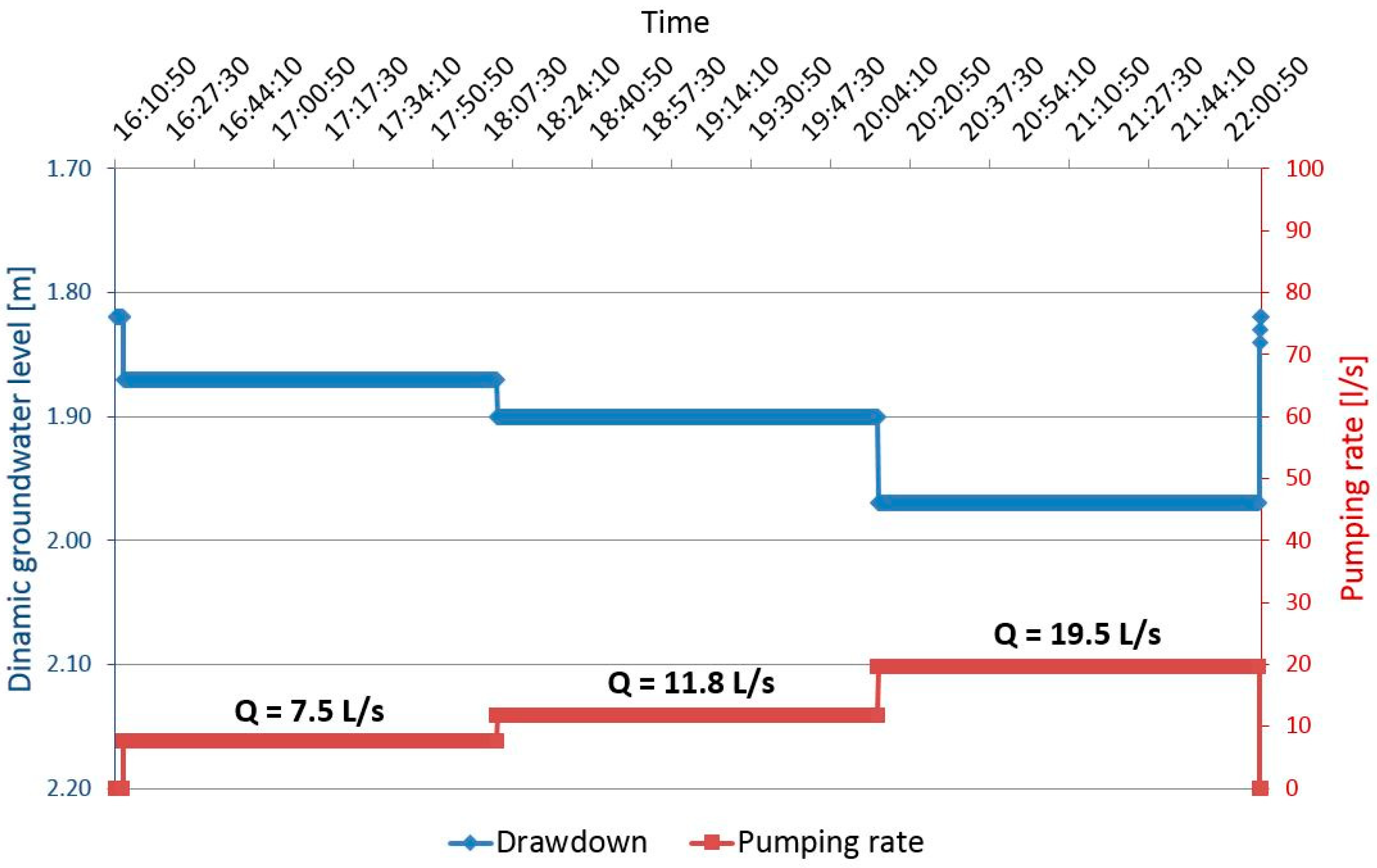
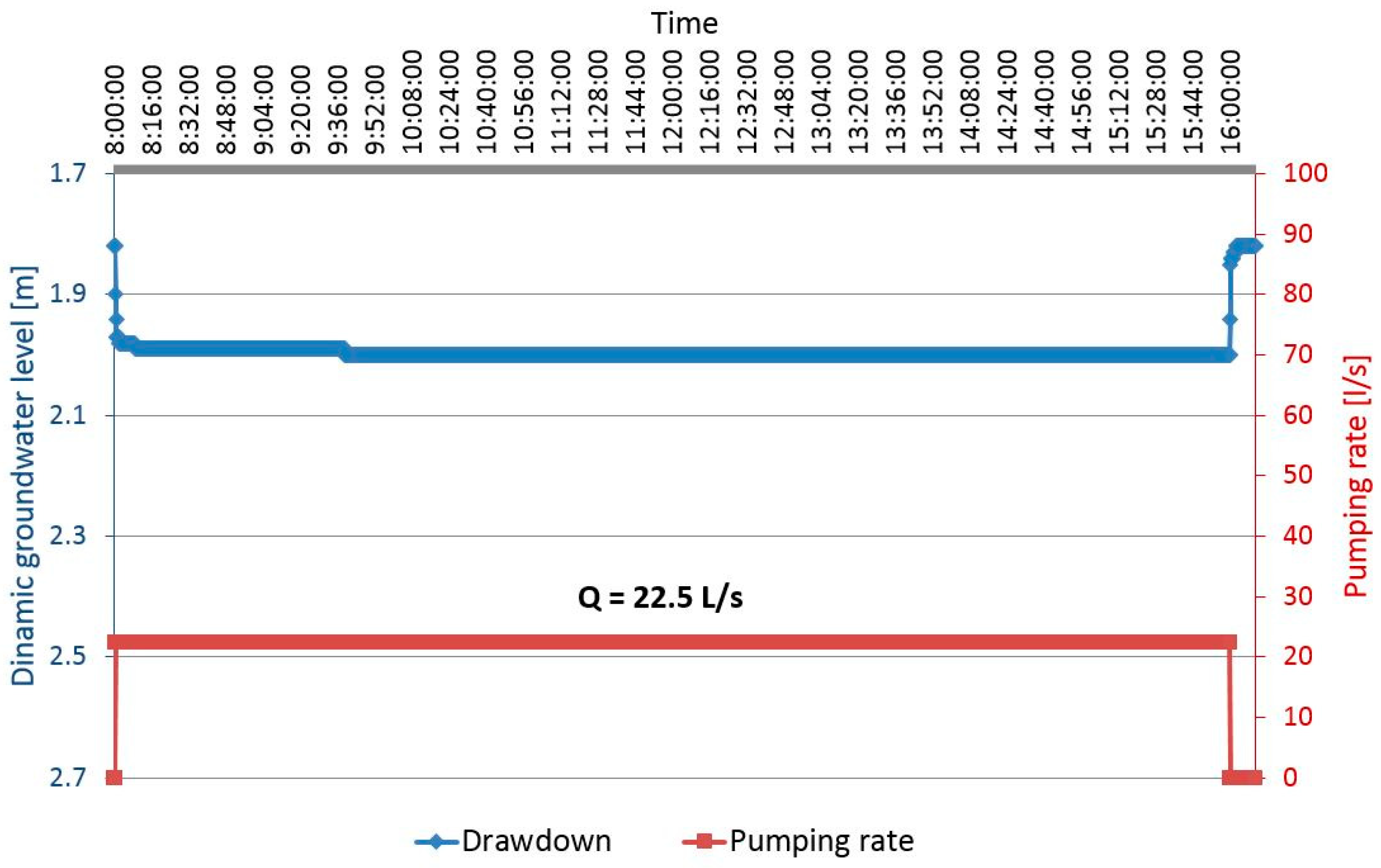
2.2. Pumping Tests
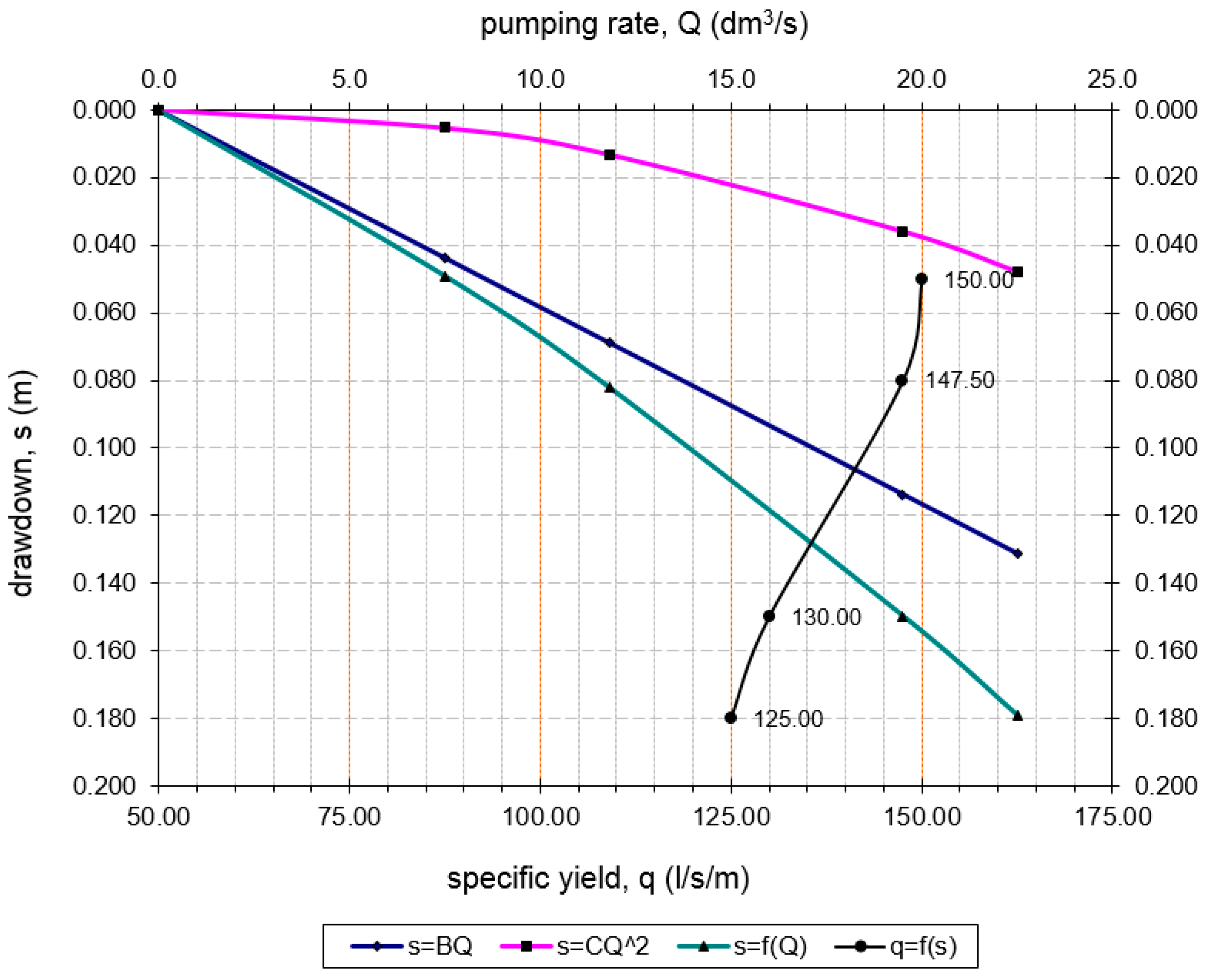
- st—total drawdown in a pumping well (m);
- sa = BQ—part of drawdown due to Aquifer losses, as laminar term;
- sw = CQ2—part of drawdown due to well losses, as turbulent term;
- B—factor related to the hydraulic characteristics of the aquifer (s/m2);
- C—factor related to the characteristics of the well (s2/m5);
- Q—pumping rate (m3/s).
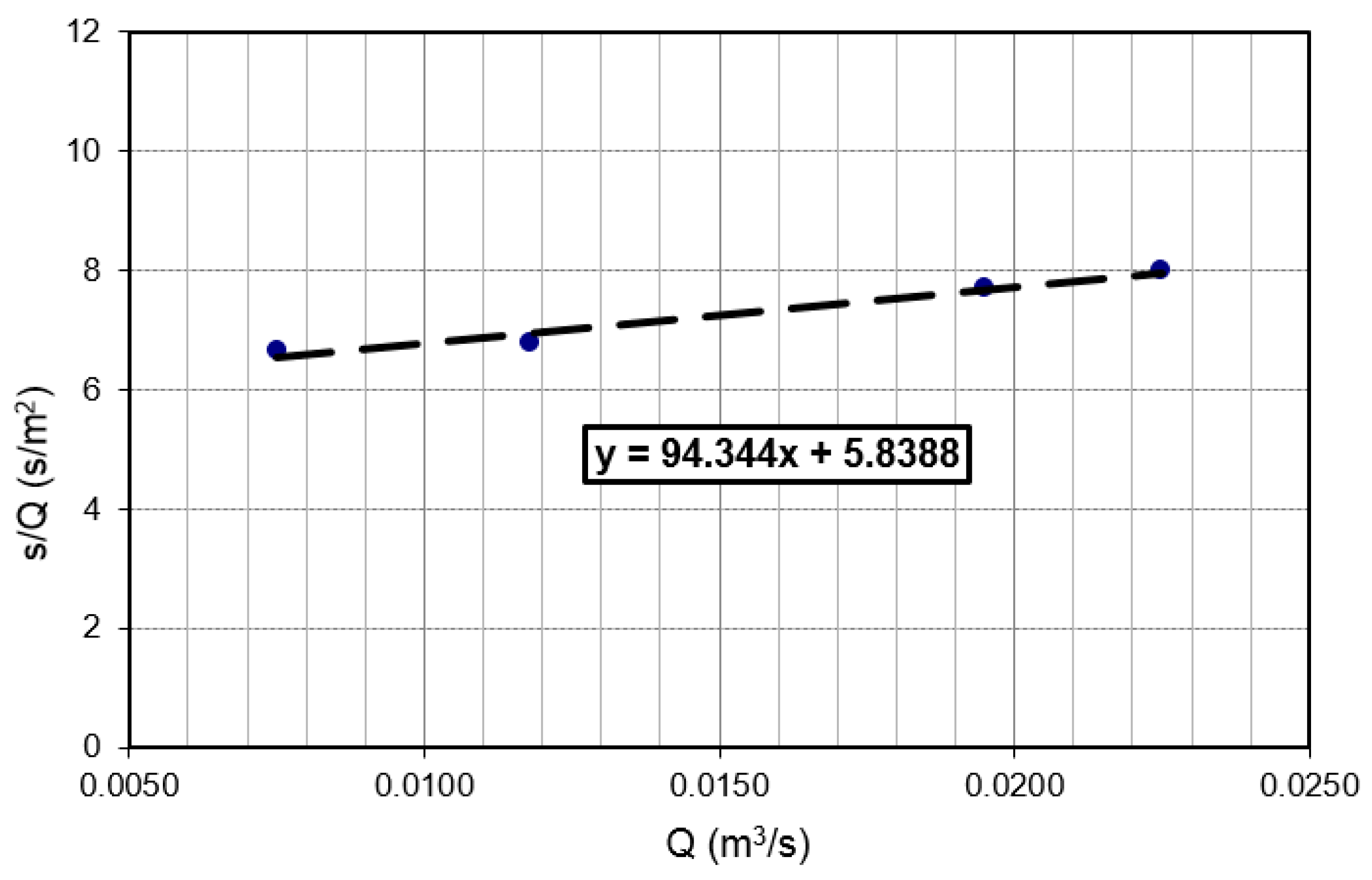
- Draw for up to more different Q, find sT based on the well equation st = BQ + CQ2.
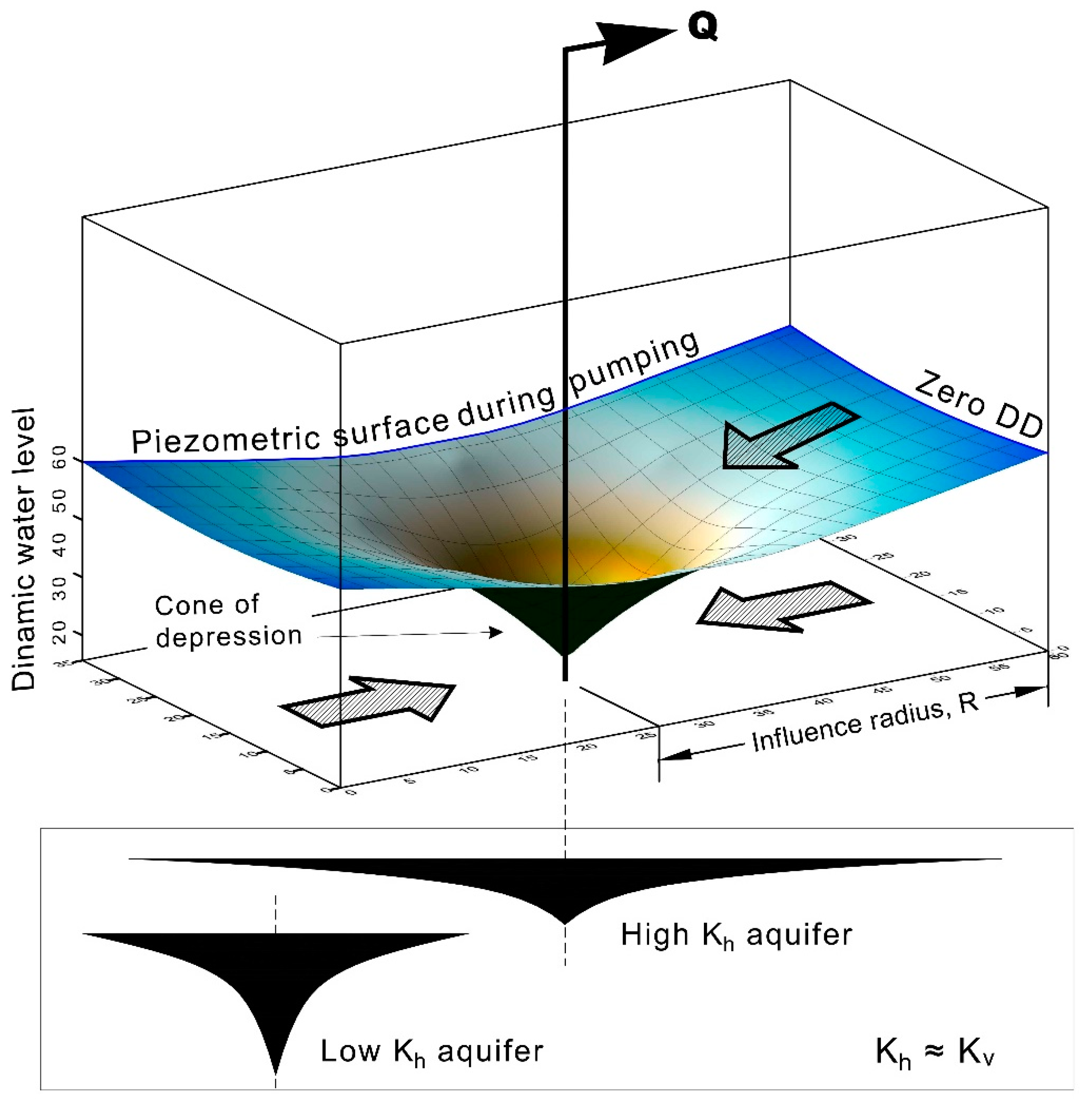
- For the same pumping rates, find theoretical (s) through the equation: s = (q/2πk) ln(R/rw), Figure 4.
- Calculate well efficiency for all pumping rates.
- Display the graph between efficiencies and pumping rates, and choose a Q value that corresponds to more than 65% efficiency or more.
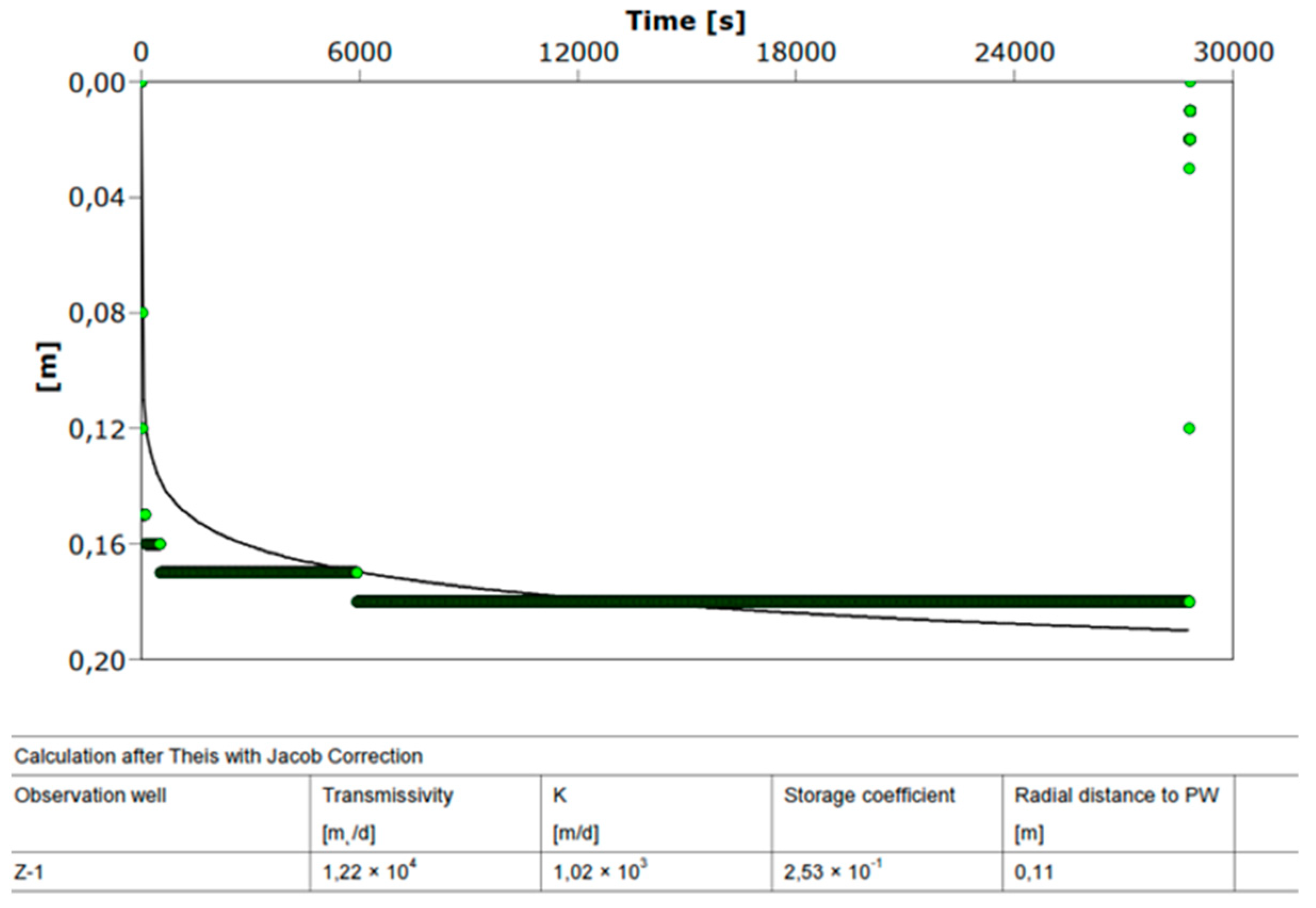
- R—influence radius (m); T—transmissivity (m/s); t—time (s); S—storage.
- h—height of the water table above substratum (m); n—effective porosity.
- k—hydraulic conductivity (m/s); s—drawdown in the borehole (m).
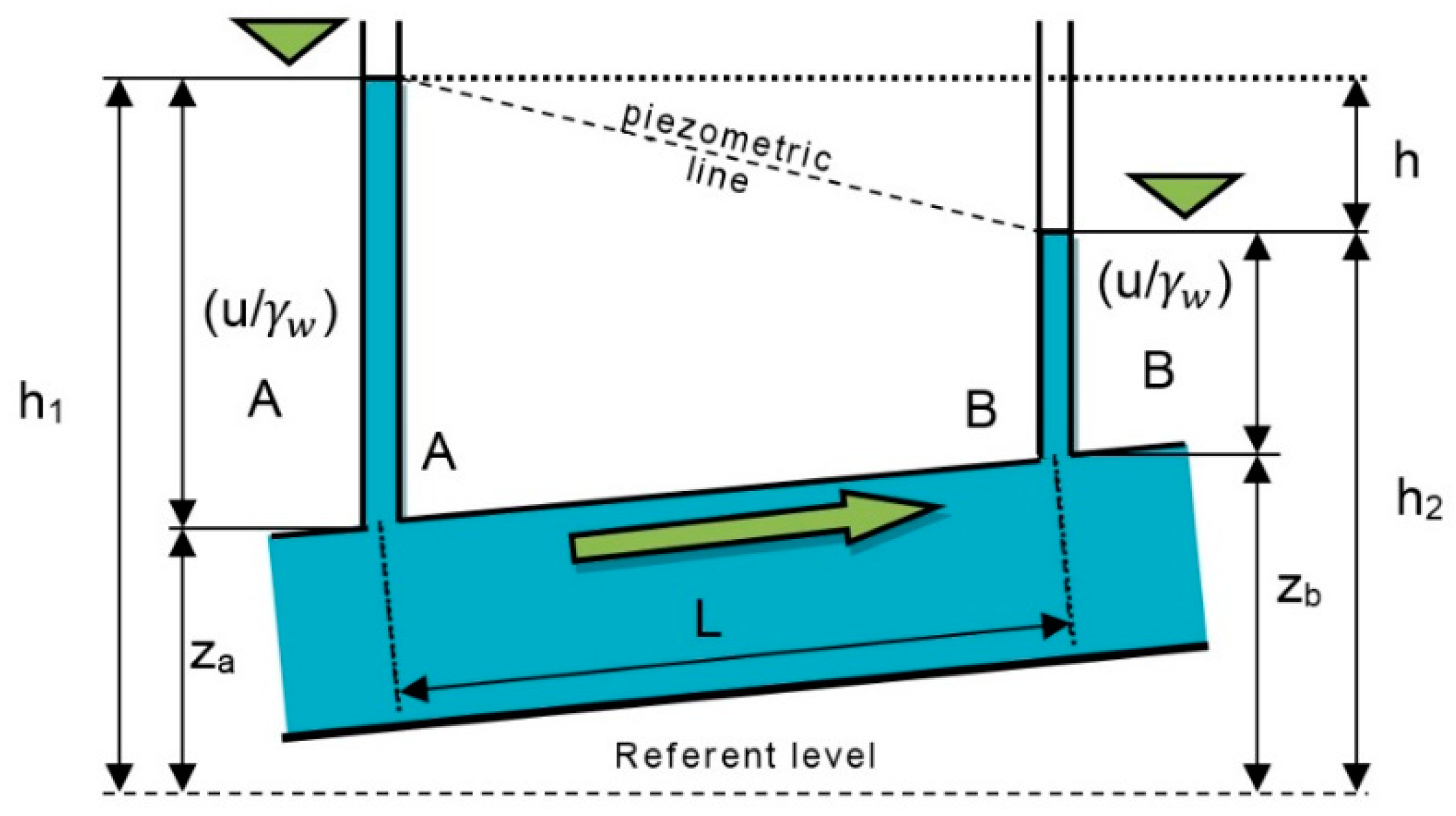
2.3. Velocity of Groundwater Flow Rate (Darcy’s Law)
- v—Darcy velocity of flow (m/s);
- Q—volume of water passing through the porous medium per unit time (m3/s);
- A—cross-sectional area of the porous media (m2);
- k—coefficient of permeability or coefficient of hydraulic conductivity (m/s);
- i—hydraulic gradient, i = (h1 − h2)/L (−);
- L—distance between piezometers (m).
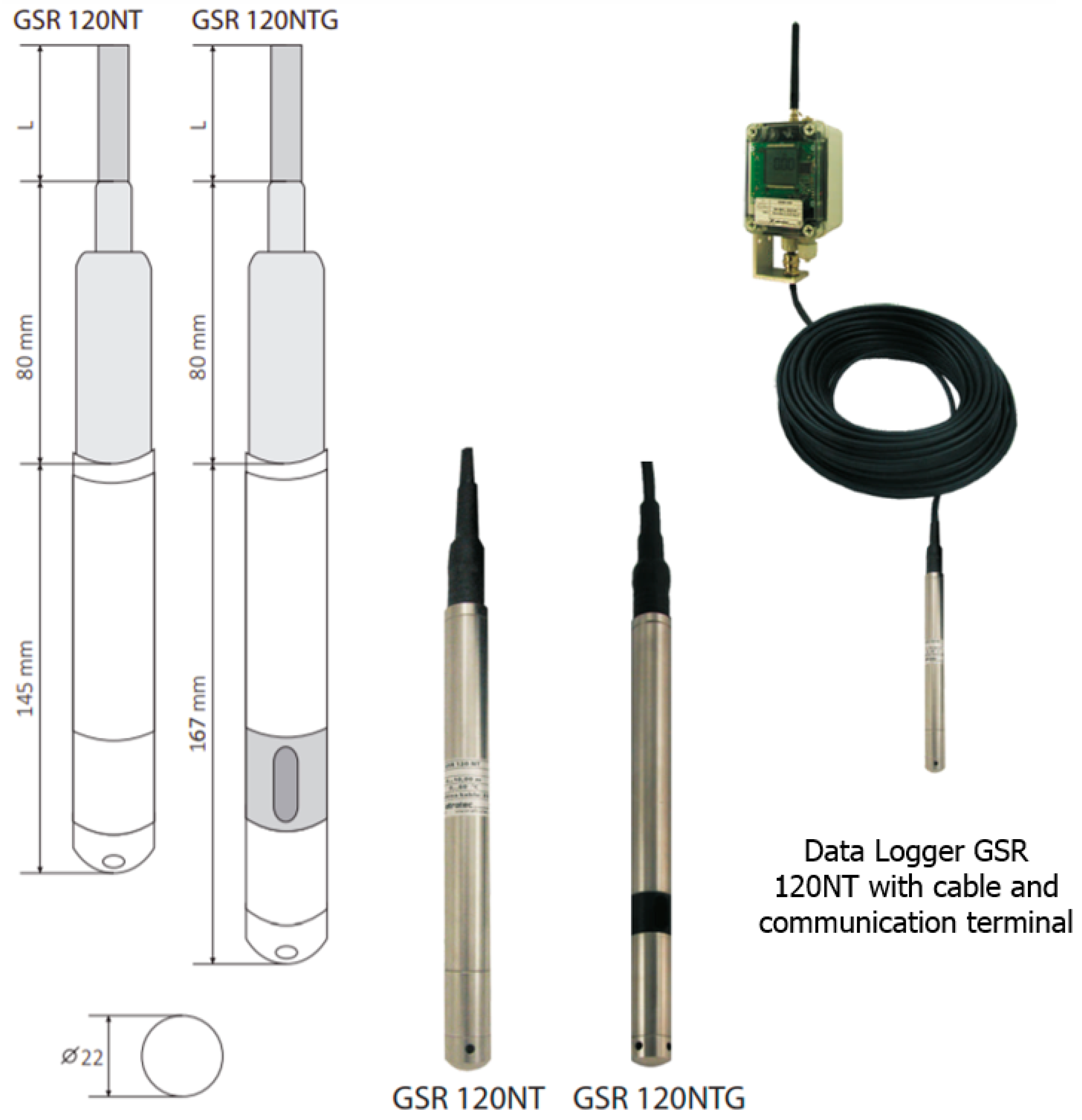
2.4. Sensors Used for the Measurements
- −
- Level, temperature, and conductivity measurements;
- −
- Compact submersible stainless steel housing;
- −
- Battery or grid powered;
- −
- Communication connection RS 485;
- −
- Data transfer and parameter settings can be done with a computer (wired connection) or over a GSM modem (wireless connection);
- −
- Easy assembly.
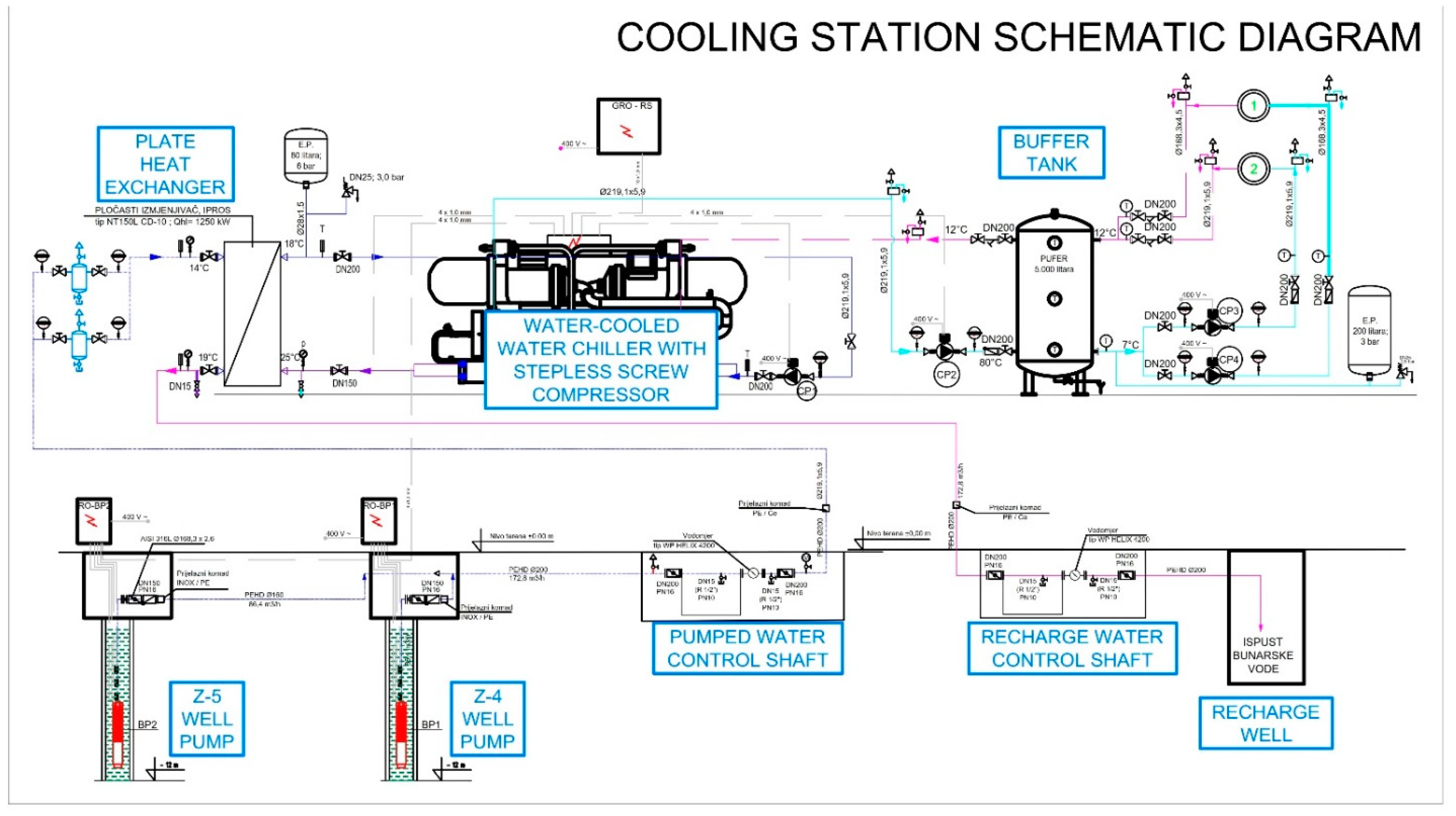
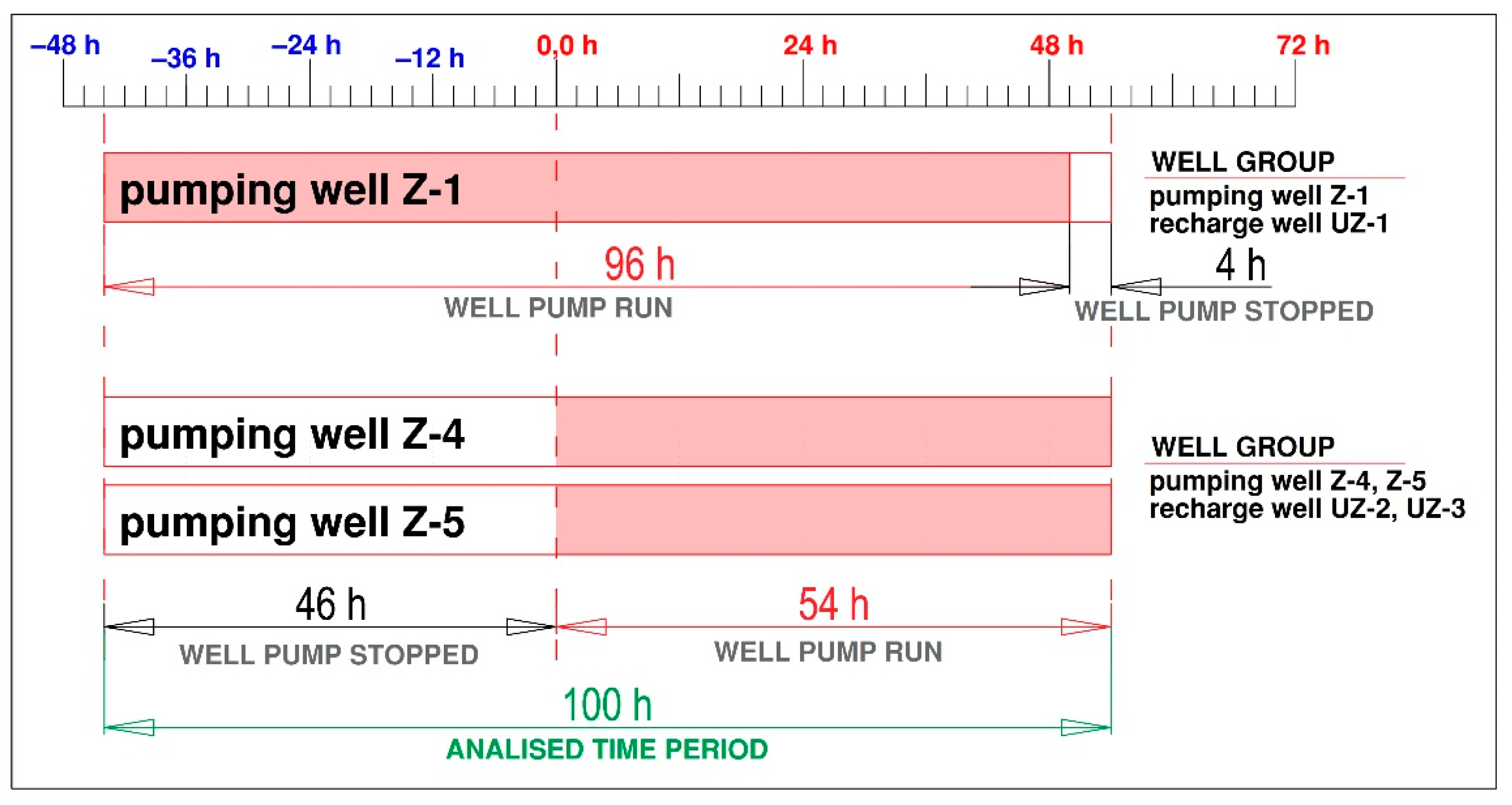
2.5. Short Description of the Operation of the Cooling Station
3. Results
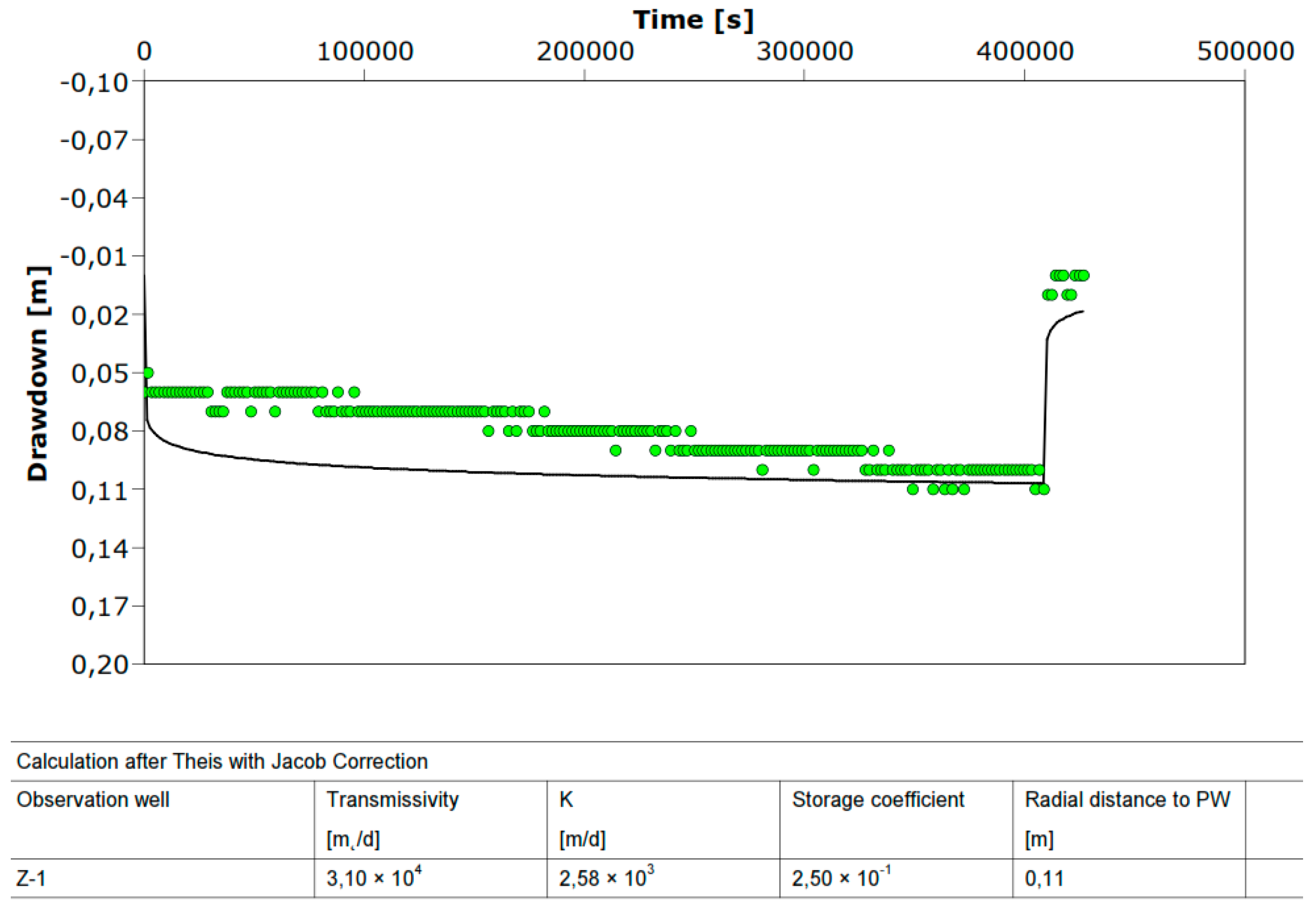
3.1. Results of Pumping Tests
3.2. Hydrogeological Aquifer Parameters
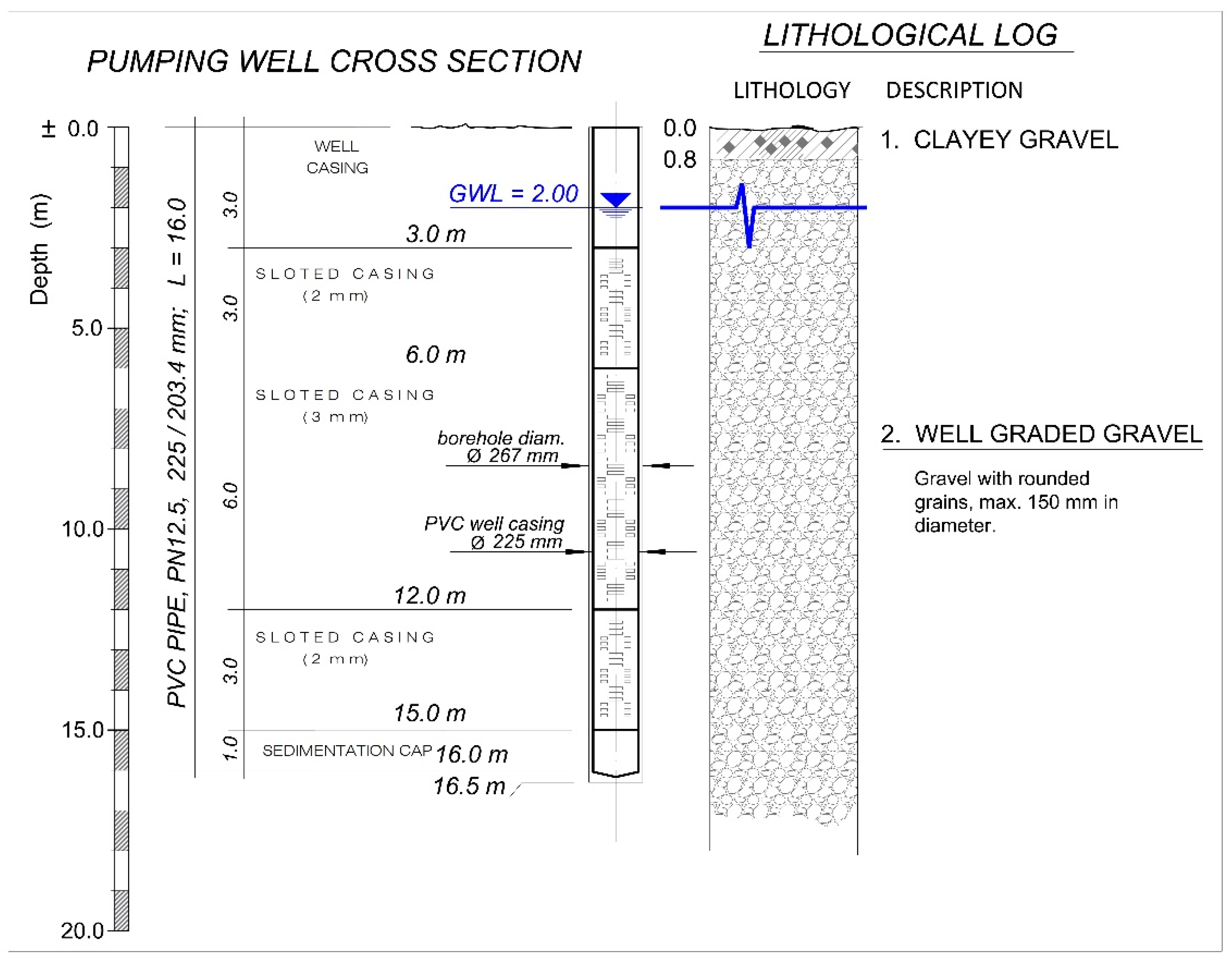
- d = 0.225 m—the diameter of the built-in filter;
- v = 0.03 m/s—maximum velocity of water entry into the filter for laminar flow conditions;
- s = 2.00 mm—the width of the strip opening (slot) of the filter;
- f = 12.70 %—total perforated (slotted) part of the filter in percentages;
- L = 12.00 m—the total length of the built-in filter;
- = 2.69 l/s—specific capacity per meter length.
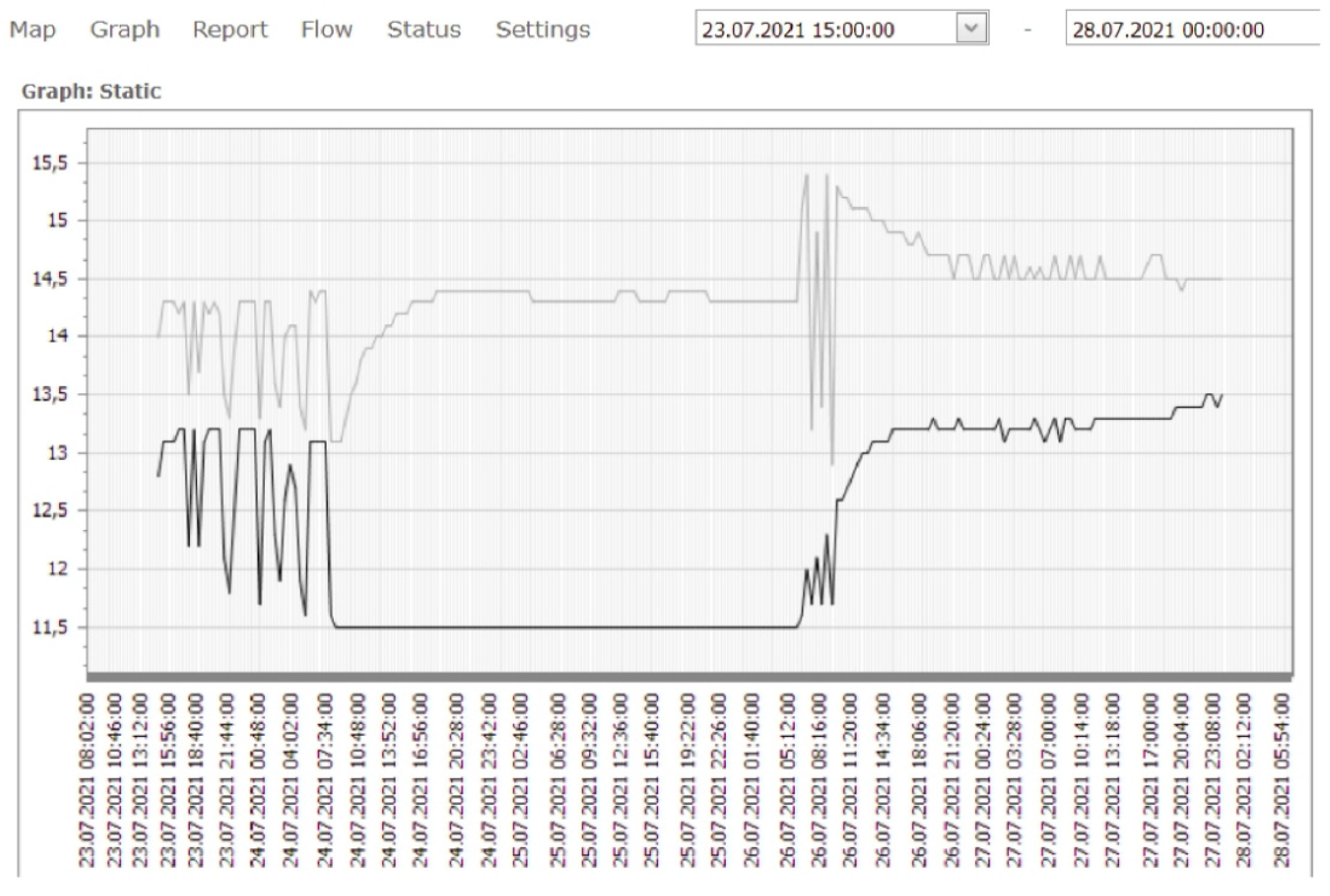
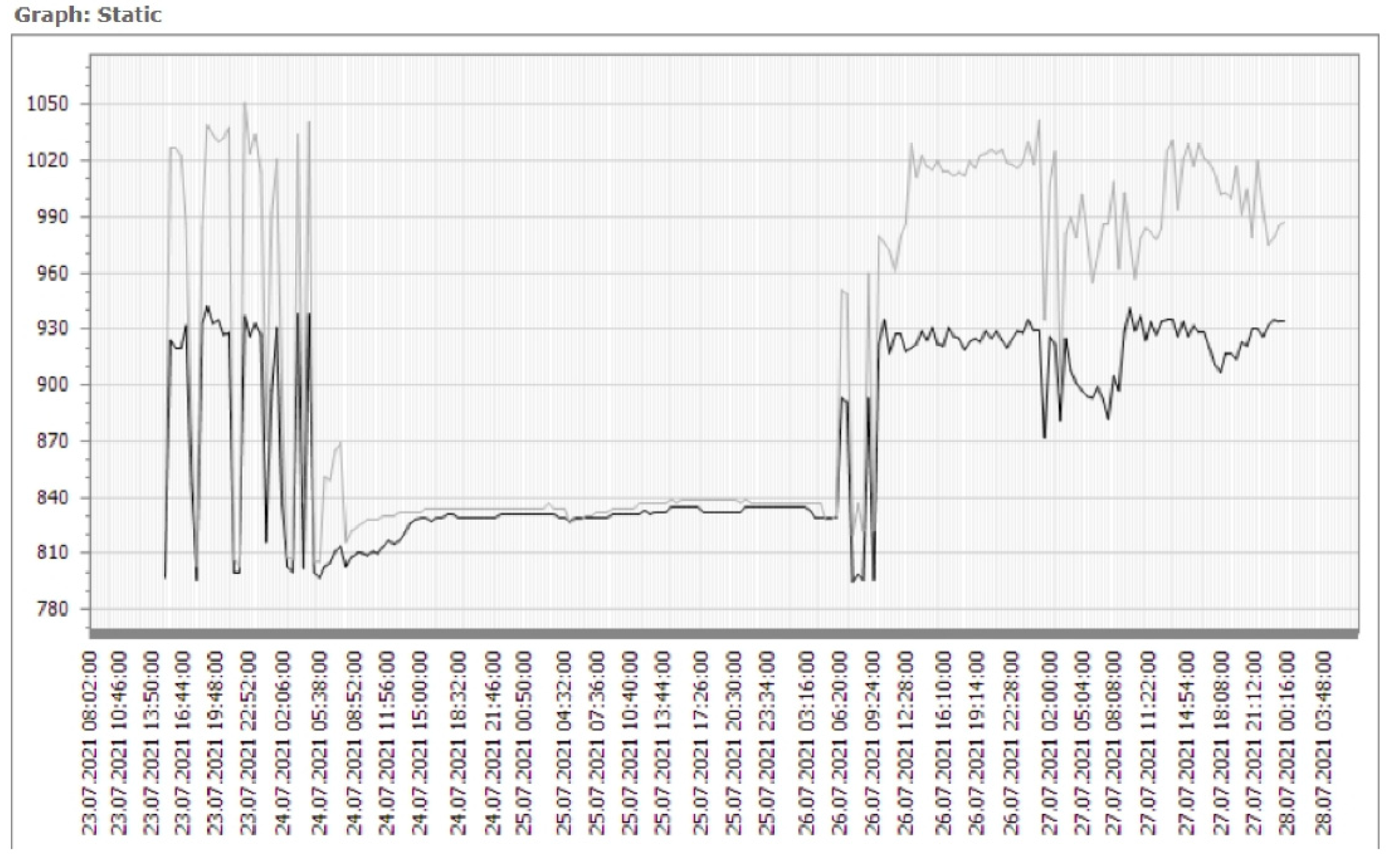
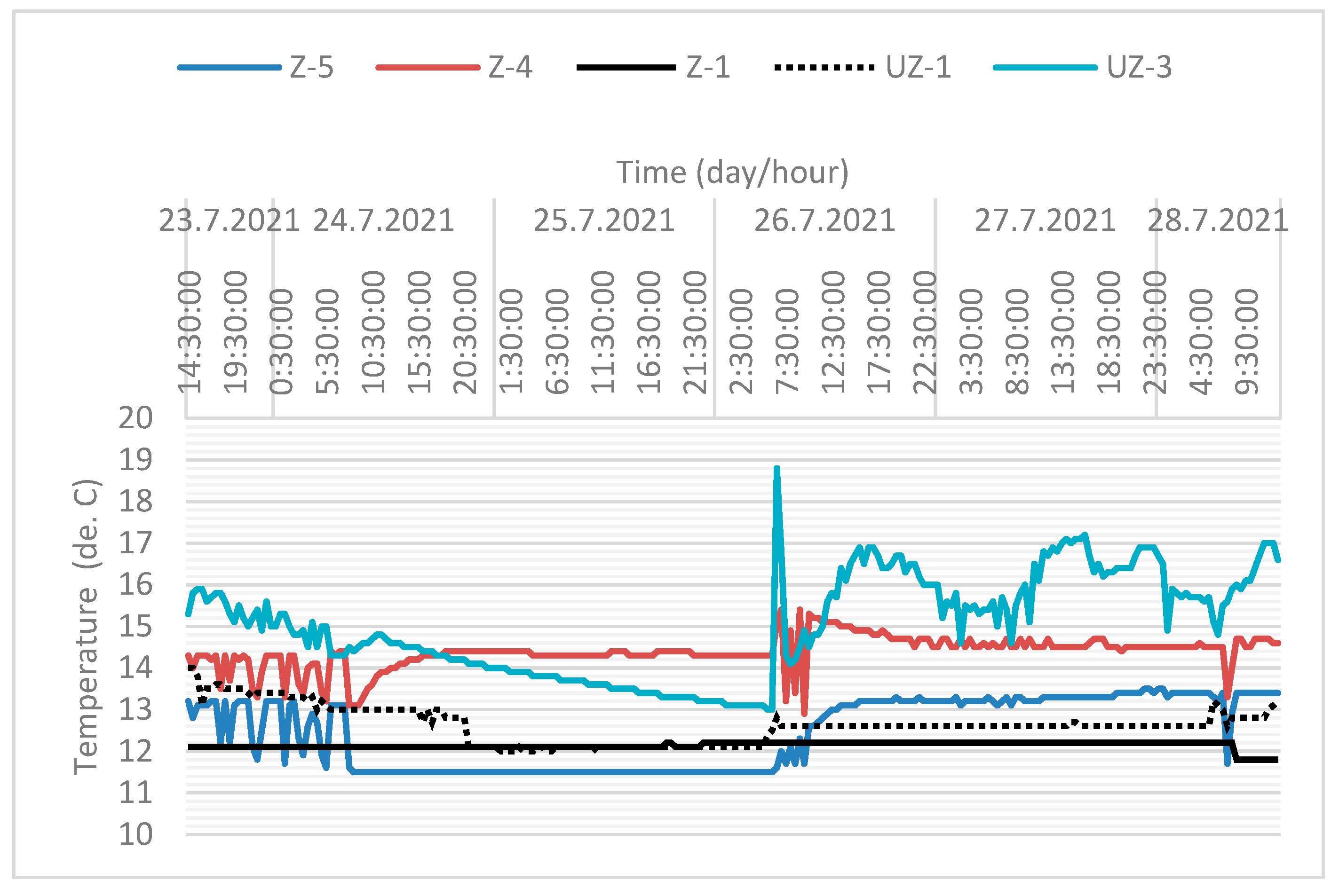
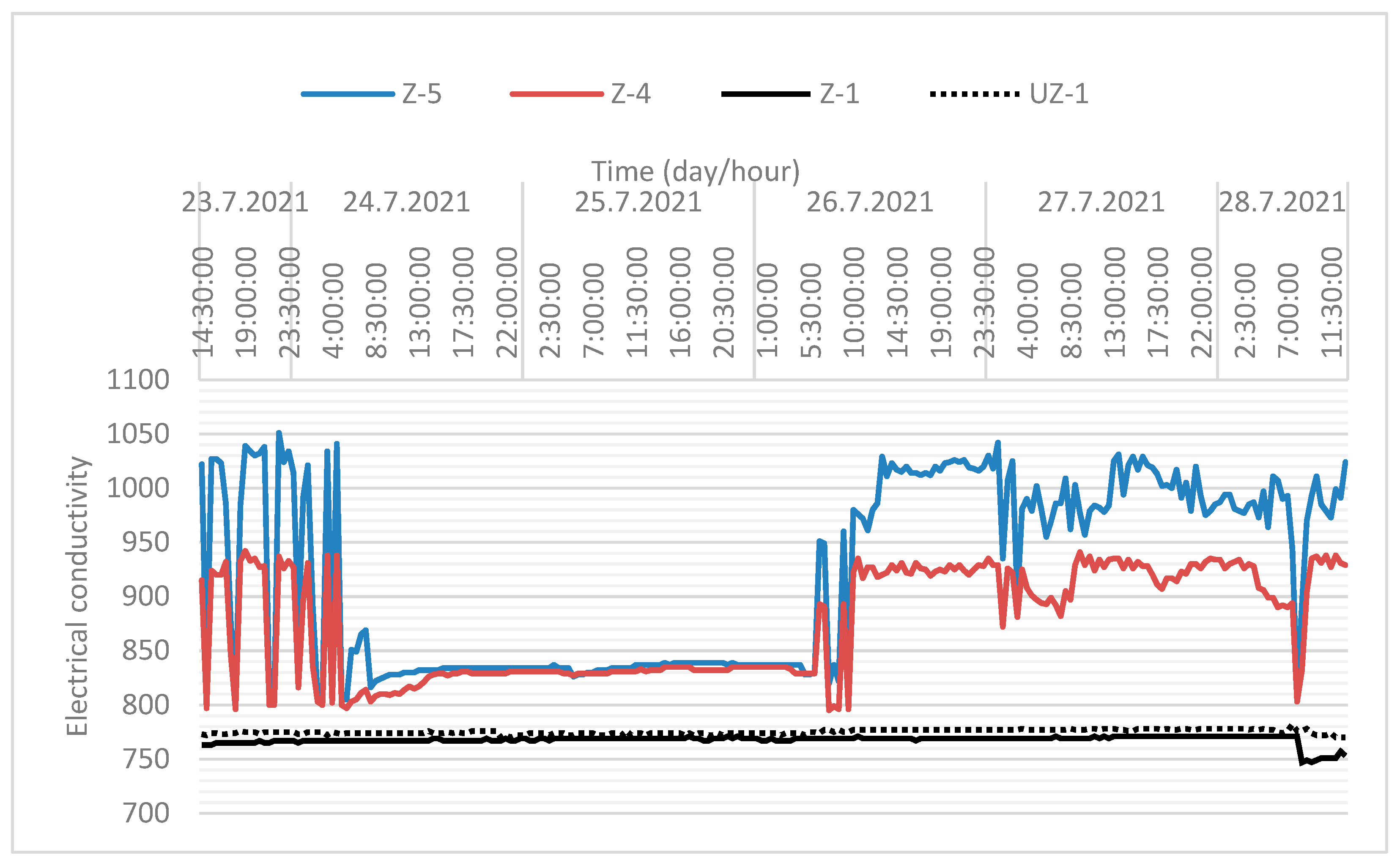
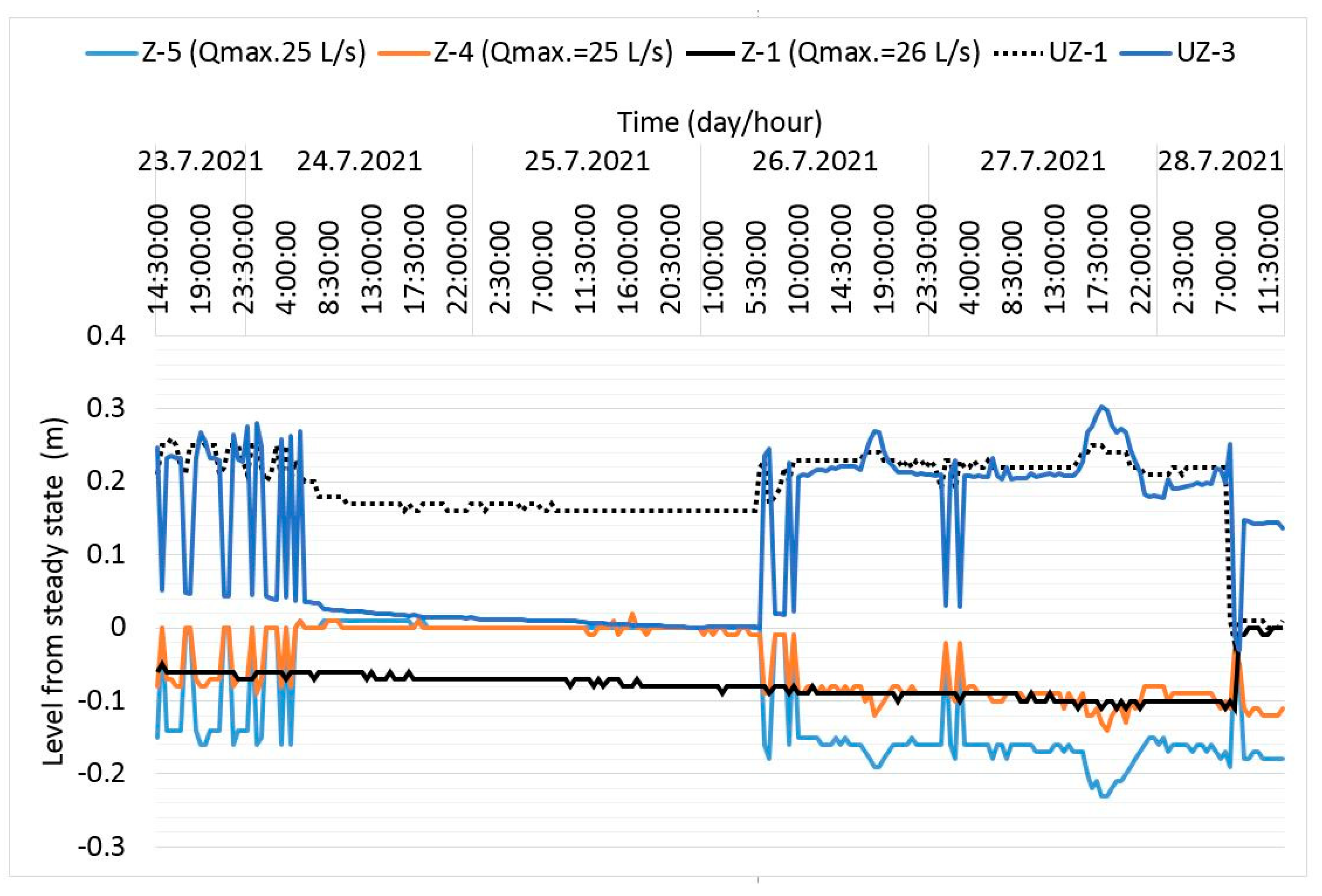
3.3. Results of Sensory Observation on Wells
4. Discussion
4.1. Analysis of Pumping Test Results
4.2. Analysis Sensors Obtained Data
5. Conclusions
Author Contributions
Funding
Institutional Review Board Statement
Informed Consent Statement
Data Availability Statement
Conflicts of Interest
References
- Garman, D.K. Geothermal Technologies Program: Buried Treasure: The Evironmental, Economic and Employment Benefits of Geothermal Energy; U.S. Department of Energy: Washington, DC, USA, 2004.
- Younis, M.; Bolisetti, T.; Ting, D.S. Ground source heat pump systems: Current status. Int. J. Environ. Stud. 2010, 67, 405–415. [Google Scholar] [CrossRef]
- Bundschuh, J.; Chen, G. (Eds.) Sustainable Energy Solutions in Agriculture, 1st ed.; CRC Press: London, UK, 2014; ISBN 9780429227493. [Google Scholar]
- Sommer, W.T.; Valstar, J.; Leusbrock, I.; Grotenhuis, J.T.C.; Rijnaarts, H.H.M. Optimization and spatial pattern of large-scale aquifer thermal energy storage. Appl. Energy 2015, 137, 322–337. [Google Scholar] [CrossRef]
- Ooka, R.; Nam, Y.; Shiba, Y.; Tanifuji, K.; Okumura, T.; Miwa, Y. Development of groundwater circulation heat pump system. HVAC&R Res. 2011, 17, 556–565. [Google Scholar] [CrossRef]
- Schout, G.; Drijver, B.; Gutierrez-Neri, M.; Schotting, R. Analysis of recovery efficiency in high-temperature aquifer thermal energy storage: A Rayleigh-based method. Hydrogeol. J. 2014, 22, 281–291. [Google Scholar] [CrossRef]
- Ganguly, S.; Mohan Kumar, M.S.; Date, A.; Akbarzadeh, A. Numerical investigation of temperature distribution and thermal performance while charging-discharging thermal energy in aquifer. Appl. Therm. Eng. 2017, 115, 756–773. [Google Scholar] [CrossRef]
- Marković, S.; Mioč, P. Basic Geological Map of SFRY 1:100000, Geology of the Nađ-Kaniža sheet; Federal Geological Institute: Belgrade, Serbia, 1989; pp. 33–58. [Google Scholar]
- Urumović, K.; Hlevnjak, B.; Prelogović, E.; Mayer, D. Hydrogeological Conditions of the Varaždin Aquifer. Geološki Vjesn. 1990, 43, 149–158. [Google Scholar]
- Confined and Unconfined Aquifers. Available online: https://dpipwe.tas.gov.au/water/groundwater/aquifers/confined-unconfined-aquifers (accessed on 20 September 2021).
- Todd, D.K.; Mays, L.W. Groundwater Hydrology, 3rd ed.; Wiley: Hoboken, NJ, USA, 2005; ISBN 978-0-471-05937-0. [Google Scholar]
- Bear, J. Dynamics of Fluids in Porous Media. Soil Sci. 1972, 120, 162–163. [Google Scholar] [CrossRef] [Green Version]
- Freeze, R.A.; Cherry, J.A. Groundwater; Prentice-Hall, Inc.: Upper Saddle River, NJ, USA, 1979; ISBN 9780133653120. [Google Scholar]
- Kruseman, G.P.; de Ridder, N.A.; Ridder, N.A.; Verweij, J.M. Improvement Analysis and Evaluation of Pumping Test Data; ILRI publication; International Institute for Land Reclamation and Improvement: Wageningen, The Netherlands, 1990; ISBN 9789070754204. [Google Scholar]
- Hydrogeologic, W. Aquifer Test. Available online: https://www.waterloohydrogeologic.com/products/aquifertest/ (accessed on 20 September 2021).
- Heath, R.C. Basic ground-water hydrology. In Geological Survey Water-Supply Paper; U.S. Geological Survey: Reston, VA, USA, 1983. [Google Scholar]
- Driscoll, F.G. Groundwater and Wells; Johnson Screens: Saint Paul, MN, USA, 1986; ISBN 0-9616456-0-1. [Google Scholar]
- Jacob, C.E. Flow of Groundwater in Engineering Hydraulic; John Wiley & Sons: New York, NY, USA, 1950. [Google Scholar]
- Fetter, C.W. Applied Hydrogeology; Maxwell Macmillan International: Long grove, IL, USA, 1994; ISBN 978-93-893-9654-6. [Google Scholar]
- Walton, W.C. Groundwater resource evaluation. J. Hydrol. 1971, 14, 363. [Google Scholar] [CrossRef]
- Fileccia, A. Some simple procedures for the calculation of the influence radius and well head protection areas (theoretical approach and a field case for a water table aquifer in an alluvial plain). Acque Sotter. Ital. J. Groundw. 2015, 4, 7–23. [Google Scholar] [CrossRef]
- Copper, H.H.; Jacob, C.E. A generalized graphical method for evaluating formation constants and summarizing well-field history. Eos. Trans. Am. Geophys. Union 1946, 27, 526–534. [Google Scholar] [CrossRef]
- Aravin, V.I.; Numerov, S.N. Theory of motion of liquids and gases in undeformable porous media. Gostekhizdat Mosc. 1953, 616. [Google Scholar]
- Cashman, P.M.; Preene, M. Groundwater Lowering in Construction; Spon Press: London, UK, 2001; ISBN 0-419-21110-1. [Google Scholar]
- Darcy, H. Les Fontaines Publiques de la Ville de Dijon: Exposition et Application; Victor Dalmont: Paris, France, 1856. [Google Scholar]
- Fetter, C.W. Contaminant Hydrogeology; Maxwell Macmillan International: New York, NY, USA, 1993; ISBN 0023371358. [Google Scholar]
- Domenico, P.A.; Schwartz, F.W. Physical and Chemical Hydrogeology. Geol. Mag. 1991, 128, 681–682. [Google Scholar] [CrossRef]
- Hall, S.; Luttrell, S.; Cronin, W.E. Method for estimating effective porosity and ground-water velocity. Groundwater 1991, 29, 171–174. [Google Scholar] [CrossRef]
- Norton, D. Transport Phenomena in Hydrothermal Systems: The redistribution of Chemical Components around Cooling Magmas. Bulletin de Minéralogie 1979, 102, 471–486. [Google Scholar] [CrossRef]
- Peyton, G.; Gibb, J.; LeFaivre, M.; Ritchey, J. On the concept of effective porosity and its measurement in saturated fine-grained porous materials. In Proceedings of the 2nd Canadian/American Conference of Hydrology, Banff, AB, Canada, 25–29 June 1985. [Google Scholar]
- Stephens, D.B.; Hsu, K.-C.; Prieksat, M.A.; Ankeny, M.D.; Blandford, N.; Roth, T.L.; Kelsey, J.A.; Whitworth, J.R. A comparison of estimated and calculated effective porosity. Hydrogeol. J. 1998, 6, 156–165. [Google Scholar] [CrossRef]
- Muckenthaler, P. Hydraulische Sicherheit von Staudämmen; Technical University: München, Germany, 1989. [Google Scholar]


| Well Loss C (min2/m5) | Well Conditions |
|---|---|
| <0.5 | Good design and yield |
| 0.5–1.0 | Medium losses due to colmation |
| 1.0–4.0 | Seriously impaired due to colmation |
| >4.0 | Very hard to regenerate to its original state |
| Well | Well Coordinates (HTRS96/TM) | GWL (Relatively) | GWL (Absolutely) | Well Distance (m) | ΔGWL (m) | i (-) | |||
|---|---|---|---|---|---|---|---|---|---|
| E | N | H | i (-) | ||||||
| Z-5 | 508,280.62 | 5,133,821.51 | 147.65 | −2.130 | 145.515 | ||||
| 27.30 | 0.0250 | 0.0009 | 0.0007 | ||||||
| Z-4 | 508,307.86 | 5,133,823.74 | 147.84 | −2.350 | 145.490 | ||||
| 164.70 | 0.1010 | 0.0006 | |||||||
| Z-1 | 508,150.29 | 5,133,871.66 | 147.55 | −1.960 | 145.591 | ||||
| 221.10 | 0.1310 | 0.0006 | |||||||
| UZ-1 | 508,371.35 | 5,133,865.71 | 147.81 | −2.350 | 145.460 | ||||
| 127.20 | 0.0088 | 0.0007 | |||||||
| Z-2 | 508,250.17 | 5,133,904.50 | 147.62 | −2.070 | 145.548 | ||||
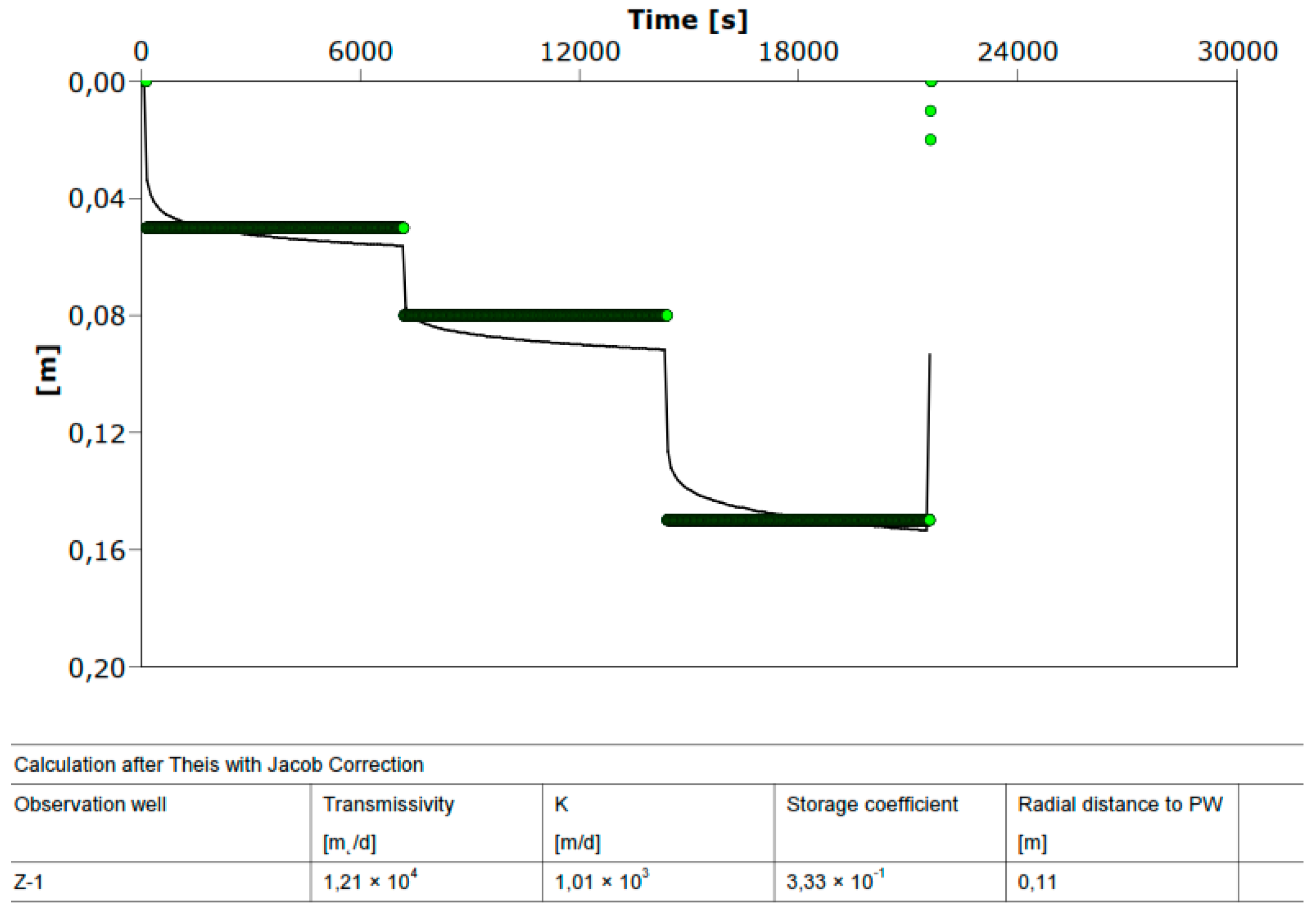
| Test | k (m/Day) | T (m2/Day) | S |
|---|---|---|---|
| Constant | 1020 | 12,200 | 0.253 |
| Step | 1010 | 12,100 | 0.330 |
| Well | Wells Coordinates (HTRS96/TM) | Q (l/s) | Drawdown/Build-Up (m) | |
|---|---|---|---|---|
| E | N | |||
| Z-1 | 508,150.28 | 5,133,871.66 | 26 | 0.12 |
| Z-2 | 508,250.17 | 5,133,904.49 | 1 | 0.04 |
| Z-3 | 508,369.00 | 5,133,940.00 | 1 | −0.05 |
| Z-4 | 508,307.86 | 5,133,823.73 | 25 | 0.09 |
| Z-5 | 508,280.62 | 5,133,821.51 | 25 | 0.12 |
| UZ-1 | 508,371.35 | 5,133,865.71 | −26 | −0.20 |
| UZ-2 | 508,375.23 | 5,133,851.64 | −25 | −0.20 |
| UZ-3 | 508,365.56 | 5,133,838.46 | −25 | −0.18 |
Publisher’s Note: MDPI stays neutral with regard to jurisdictional claims in published maps and institutional affiliations. |
© 2021 by the authors. Licensee MDPI, Basel, Switzerland. This article is an open access article distributed under the terms and conditions of the Creative Commons Attribution (CC BY) license (https://creativecommons.org/licenses/by/4.0/).
Share and Cite
Strelec, S.; Grabar, K.; Jug, J.; Kranjčić, N. Influence of Recharging Wells, Sanitary Collectors and Rain Drainage on Increase Temperature in Pumping Wells on the Groundwater Heat Pump System. Sensors 2021, 21, 7175. https://doi.org/10.3390/s21217175
Strelec S, Grabar K, Jug J, Kranjčić N. Influence of Recharging Wells, Sanitary Collectors and Rain Drainage on Increase Temperature in Pumping Wells on the Groundwater Heat Pump System. Sensors. 2021; 21(21):7175. https://doi.org/10.3390/s21217175
Chicago/Turabian StyleStrelec, Stjepan, Kristijan Grabar, Jasmin Jug, and Nikola Kranjčić. 2021. "Influence of Recharging Wells, Sanitary Collectors and Rain Drainage on Increase Temperature in Pumping Wells on the Groundwater Heat Pump System" Sensors 21, no. 21: 7175. https://doi.org/10.3390/s21217175
APA StyleStrelec, S., Grabar, K., Jug, J., & Kranjčić, N. (2021). Influence of Recharging Wells, Sanitary Collectors and Rain Drainage on Increase Temperature in Pumping Wells on the Groundwater Heat Pump System. Sensors, 21(21), 7175. https://doi.org/10.3390/s21217175