Effect of Spectral Signal-to-Noise Ratio on Resolution Enhancement at Surface Plasmon Resonance

Abstract
1. Introduction
2. Materials and Methods
2.1. Transfer Matrix Modeling
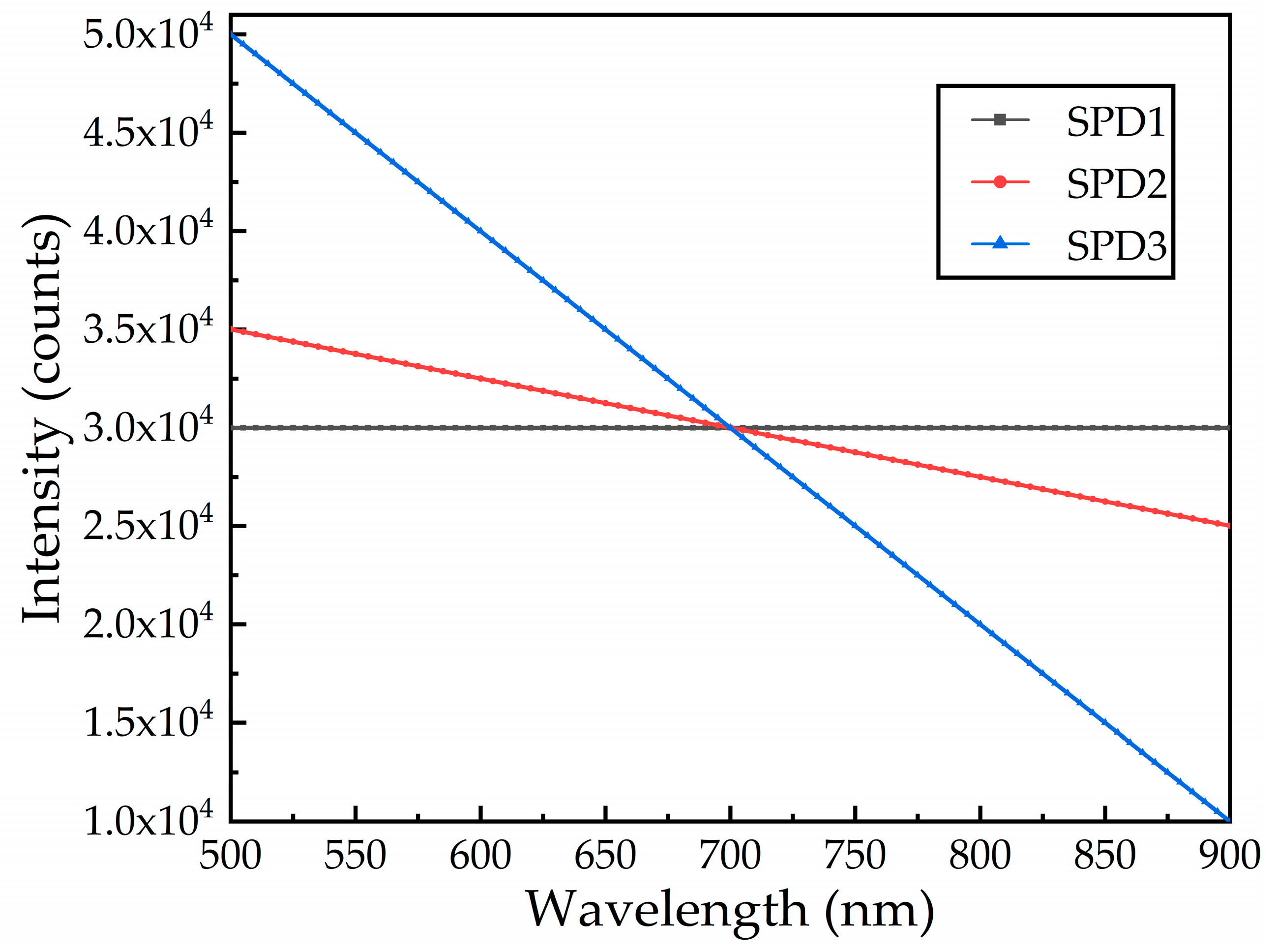
2.2. Model Parameters
2.3. RI Resolution
2.3.1. Same Noise Levels at Different SPDs
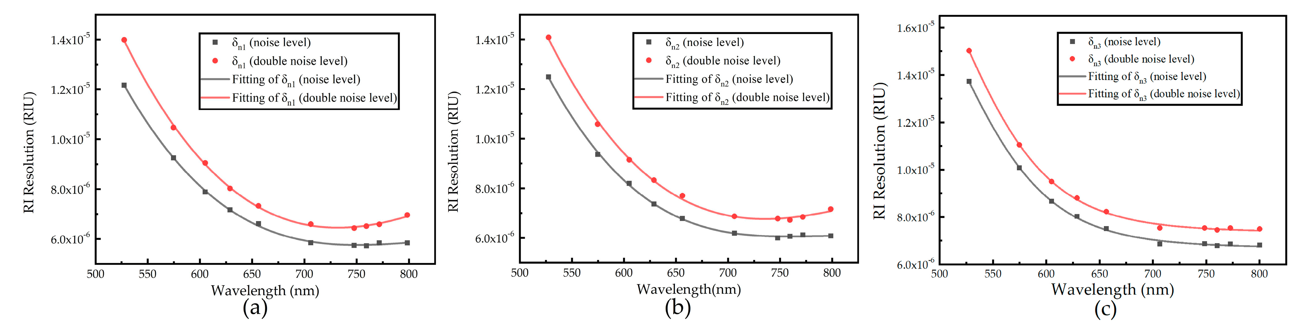
2.3.2. Same SPD at Different Noise Levels
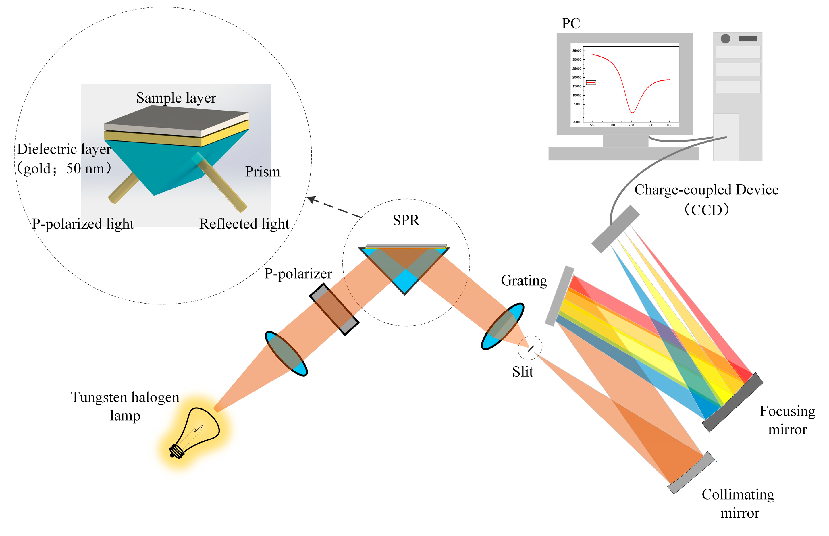
2.4. Experimental
3. Results and Discussion
3.1. Simulation Results
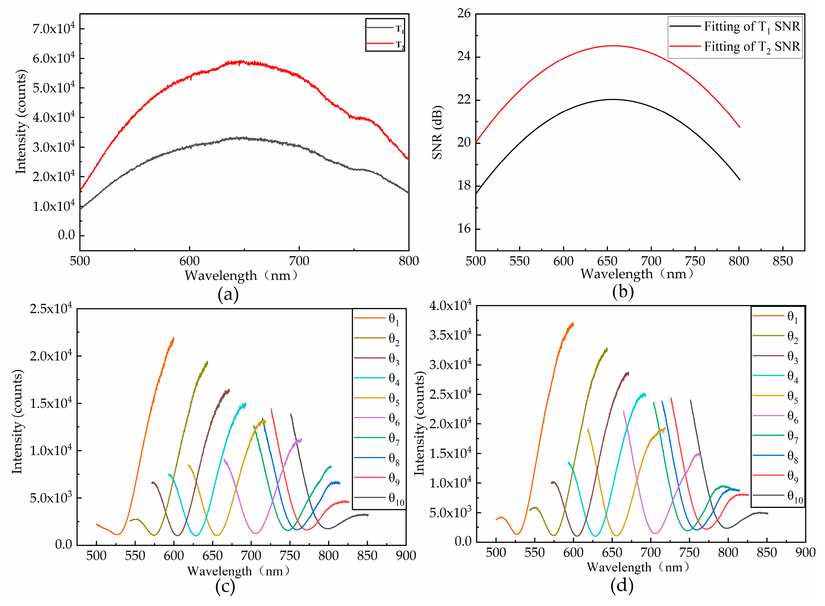
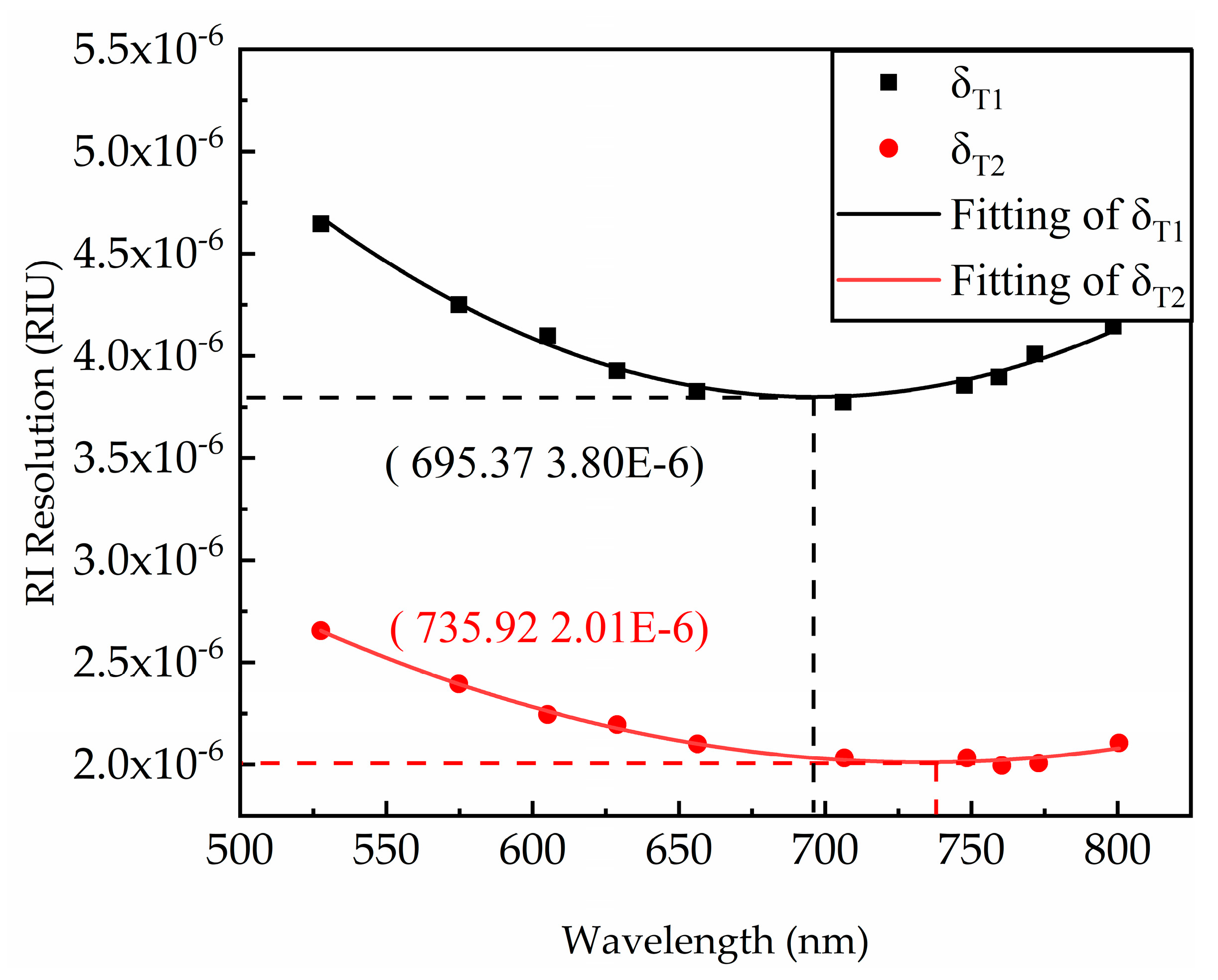
3.2. Experimental Results
3.3. Discussion
4. Conclusions
Author Contributions
Funding
Institutional Review Board Statement
Informed Consent Statement
Data Availability Statement
Conflicts of Interest
References
- Loo, F.C.; Ng, S.P.; Wu, C.M.L.; Kong, S.K. An aptasensor using DNA aptamer and white light common-path SPR spectral interferometry to detect cytochrome-c for anti-cancer drug screening. Sens. Actuators B: Chem. 2014, 198, 416–423. [Google Scholar] [CrossRef]
- Chung, J.W.; Kim, S.D.; Bernhardt, R.; Pyun, J.C. Application of SPR biosensor for medical diagnostics of human hepatitis B virus (hHBV). Sens. Actuators B: Chem. 2005, 111, 416–422. [Google Scholar] [CrossRef]
- Rasooly, A. Surface plasmon resonance analysis of staphylococcal enterotoxin B in food. J. Food Prot. 2001, 64, 37–43. [Google Scholar] [CrossRef] [PubMed]
- Conteduca, D.; Dell’Olio, F.; Innone, F.; Ciminelli, C.; Armenise, M.N. Rigorous design of an ultra-high Q/V photonic/plasmonic cavity to be used in biosensing applications. Opt. Laser Technol. 2016, 77, 151–161. [Google Scholar] [CrossRef]
- Hu, C.; Gan, N.; Chen, Y.; Bi, L.; Zhang, X.; Song, L. Detection of microcystins in environmental samples using surface plasmon resonance biosensor. Talanta 2009, 80, 407–410. [Google Scholar] [CrossRef] [PubMed]
- Yu, P.Q.; Yang, H.; Chen, X.F.; Yi, Z.; Yao, W.T.; Chen, J.F.; Yi, Y.G.; Wu, P.H. Ultra-wideband solar absorber based on refractory titanium metal. Renew. Energy 2020, 158, 227–235. [Google Scholar] [CrossRef]
- Yi, Z.; Li, J.K.; Lin, J.C.; Qin, F.; Chen, X.F.; Yao, W.T.; Liu, Z.M.; Cheng, S.B.; Wu, P.H.; Li, H.L. Broadband polarization-insensitive and wide-angle solar energy absorber based on tungsten ring-disc array. Nanoscale 2020, 12, 23077–23083. [Google Scholar] [CrossRef]
- Li, J.K.; Chen, X.F.; Yi, Z.; Yang, H.; Tang, Y.J.; Yi, Y.; Yao, W.T.; Wang, J.Q.; Yi, Y.G. Broadband solar energy absorber based on monolayer molybdenum disulfide using tungsten elliptical arrays. Mater. Today Energy 2020, 16, 100390. [Google Scholar] [CrossRef]
- Chu, P.X.; Chen, J.X.; Xiong, Z.G.; Yi, Z. Controllable frequency conversion in the coupled time-modulated cavities with phase delay. Opt. Commun. 2020, 476, 126338. [Google Scholar] [CrossRef]
- Zhang, Y.B.; Wu, P.H.; Zhou, Z.G. Study on Temperature Adjustable Terahertz Metamaterial Absorber Based on Vanadium Dioxide. IEEE Access 2020, 8, 85154–85161. [Google Scholar] [CrossRef]
- Karamanska, R.; Clarke, J.; Blixt, O.; MacRae, J.I.; Zhang, J.Q.; Crocker, P.R.; Laurent, N.; Wright, A.; Flitsch, S.L.; Russell, D.A.; et al. Surface plasmon resonance imaging for real-time, label-free analysis of protein interactions with carbohydrate microarrays. Glycoconj. J. 2008, 25, 69–74. [Google Scholar] [CrossRef] [PubMed]
- Liedberg, B.; Nylander, C.; Lunström, I. Surface plasmon resonance for gas detection and biosensing. Sens. Actuators 1983, 4, 299–304. [Google Scholar] [CrossRef]
- Zhao, Y.; Deng, Z.; Wang, Q. Fiber optic SPR sensor for liquid concentration measurement. Sens. Actuators B: Chem. 2014, 192, 229–233. [Google Scholar] [CrossRef]
- Mivehi, L.; Bordes, R.; Holmberg, K. Adsorption of cationic gemini surfactants at solid surfaces studied by QCM-D and SPR: Effect of the rigidity of the spacer. Langmuir 2011, 27, 7549–7557. [Google Scholar] [CrossRef] [PubMed]
- Maharana, P.K.; Jha, R. Chalcogenide prism and graphene multilayer based surface plasmon resonance affinity biosensor for high performance. Sens. Actuators B: Chem. 2012, 169, 161–166. [Google Scholar] [CrossRef]
- Chiang, H.P.; Lin, J.L.; Chen, Z.W. High sensitivity surface plasmon resonance sensor based on phase interrogation at optimal incident wavelengths. Appl. Phys. Lett. 2006, 88, 141105. [Google Scholar] [CrossRef]
- Piliarik, M.; Homola, J. Surface plasmon resonance (SPR) sensors: Approaching their limits? Opt. Express 2009, 17, 16505–16517. [Google Scholar] [CrossRef]
- Yi, S.J.; Yuk, J.S.; Jung, S.H.; Zhavnerko, G.K.; Kim, Y.M.; Ha, K.S. Investigation of selective protein immobilization on charged protein array by wavelength interrogation-based SPR sensor. Mol. Cells 2003, 15, 333. [Google Scholar]
- Jiang, L.Y.; Yuan, C.; Li, Z.Y.; Su, J.; Yi, Z.; Yao, W.T.; Wu, P.H.; Liu, Z.M.; Cheng, S.B.; Pan, M. Multi-band and high-sensitivity perfect absorber based on monolayer grapheme metamaterial. Diam. Relat. Mater. 2021, 111, 108227. [Google Scholar] [CrossRef]
- Zhang, Y.B.; Yi, Z.; Wang, X.Y.; Chu, P.X.; Yao, W.T.; Zhou, Z.G.; Cheng, S.B.; Liu, Z.M.; Wu, P.H.; Pan, M.; et al. Dual band visible metamaterial absorbers based on four identical ring patches. Phys. E: Low-Dimens. Syst. Nanostruct. 2020, 114526. [Google Scholar] [CrossRef]
- Cen, C.L.; Chen, Z.Q.; Xu, D.Y.; Jiang, L.Y.; Chen, X.F.; Yi, Z.; Wu, P.H.; Li, G.F.; Yi, Y. High Quality Factor, High Sensitivity Metamaterial Graphene-Perfect Absorber Based on Critical Coupling Theory and Impedance Matching. Nanomaterials 2020, 10, 95. [Google Scholar] [CrossRef]
- Chen, Z.; Liu, L.; He, Y.; Ma, H. Resolution enhancement of surface plasmon resonance sensors with spectral interrogation: Resonant wavelength considerations. Appl. Opt. 2016, 55, 884–891. [Google Scholar] [CrossRef] [PubMed]
- Maharana, P.K.; Srivastava, T.; Jha, R. On the performance of highly sensitive and accurate graphene-on-aluminum and silicon-based SPR biosensor for visible and near infrared. Plasmonics 2014, 9, 1113–1120. [Google Scholar] [CrossRef]
- Caucheteur, C.; Shevchenko, Y.; Shao, L.; Wuilpart, M.; Albert, J. High resolution interrogation of tilted fiber grating SPR sen-sors from polarization properties measurement. Opt. Express 2011, 19, 1656–1664. [Google Scholar] [CrossRef] [PubMed]
- Vlček, J.; Pištora, J.; Lesňák, M. Design of Plasmonic-Waveguiding Structures for Sensor Applications. Nanomaterials 2019, 9, 1227. [Google Scholar] [CrossRef] [PubMed]
- Cuixia, Z.; Guo, X.; Guodong, W.; Shiqun, J. Effect of Spectral Power Distribution on the Resolution Enhancement in Surface Plasmon Resonance. Photonic Sens. 2018, 8, 310–319. [Google Scholar]
- Ouyang, Q.; Zeng, S.; Jiang, L.; Hong, L.; Xu, G.; Dinh, X.Q.; Qian, J.; He, S.; Qu, J.; Coquet, P.; et al. Sensitivity Enhancement of Transition Metal Dichalcogenides/Silicon Nanostructure-based Surface Plasmon Resonance Biosensor. Sci. Rep. 2016, 6, 28190. [Google Scholar] [CrossRef]
- Xia, G.; Zhou, C.; Jin, S.; Huang, C.; Xing, J.; Liu, Z. Sensitivity Enhancement of Two-Dimensional Materials Based on Genetic Optimization in Surface Plasmon Resonance. Sensors 2019, 19, 1198. [Google Scholar] [CrossRef]
- Chan, H.; Guo, X.; Shiqun, J.; Mingyong, H.; Su, W.; Jinyu, X. Denoising analysis of compact CCD-based spectrometer. Optik 2018, 157, 693–706. [Google Scholar]
- Homola, J. On the sensitivity of surface plasmon resonance sensors with spectral interrogation. Sens. Actuators B Chem. 1997, 41, 207–211. [Google Scholar] [CrossRef]
- Rahman, M.S.; Anower, S.; Hasan, R.; Hossain, B.; Haque, I. Design and numerical analysis of highly sensitive Au-MoS 2 -graphene based hybrid surface plasmon resonance biosensor. Opt. Commun. 2017, 396, 36–43. [Google Scholar] [CrossRef]


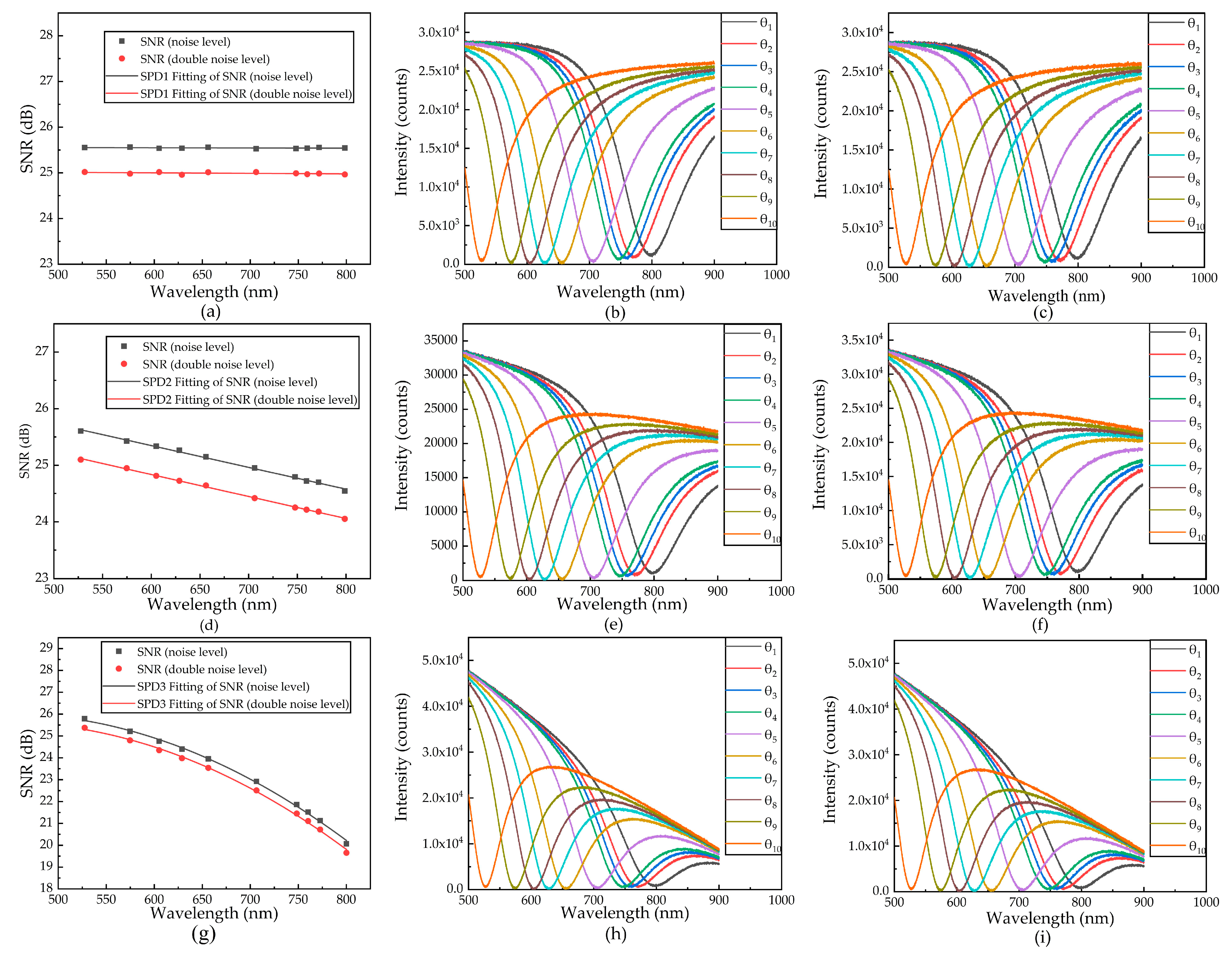
| Spectral Power Distribution | Optimal Resonance Wavelength (nm) | Best RI Resolution (RIU) | |
|---|---|---|---|
| Noise level | SPD1 | 759.30 | 5.72 × 10⁻⁶ |
| SPD2 | 795.15 | 6.08 × 10⁻⁶ | |
| SPD3 | 798.23 | 6.78 × 10⁻⁶ | |
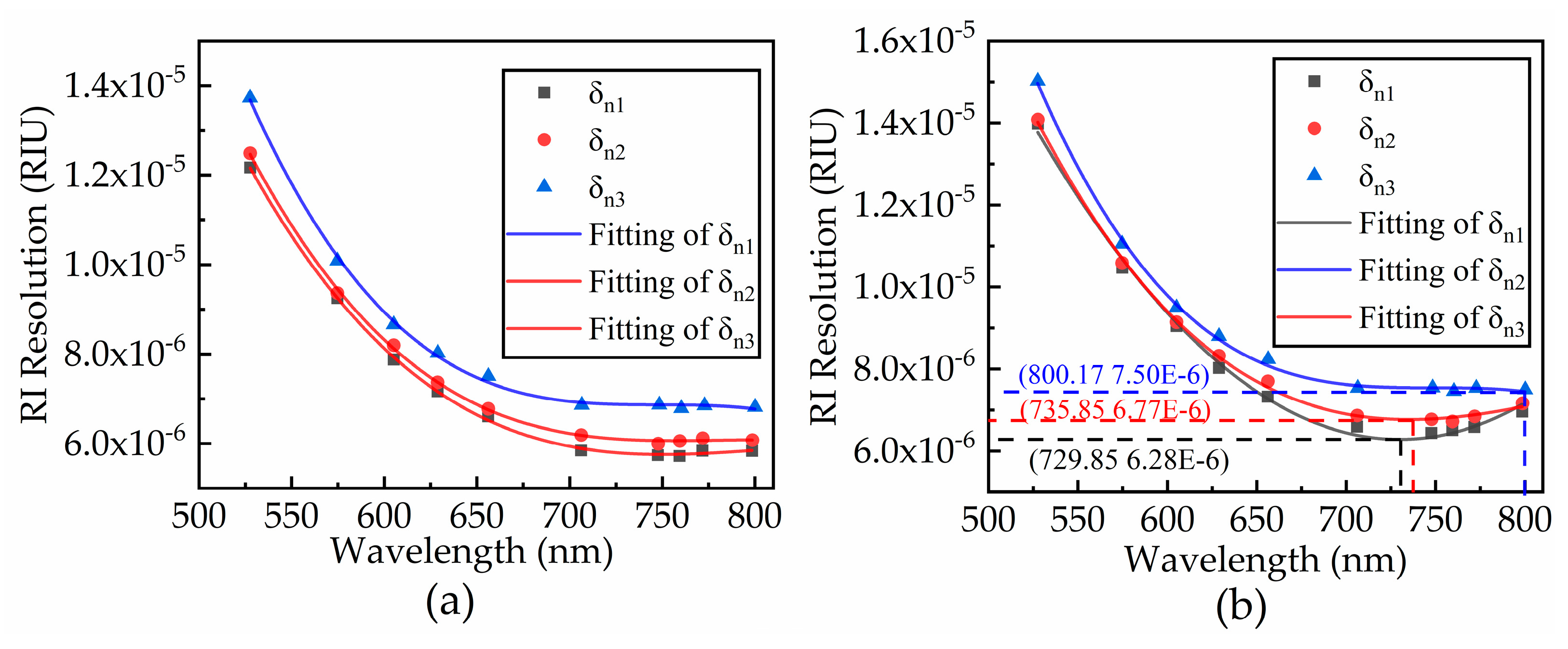
| Double Noise level | SPD1 | 729.85 | 6.28 × 10⁻⁶ |
| SPD2 | 735.85 | 6.77 × 10⁻⁶ | |
| SPD3 | 800.17 | 7.50 × 10⁻⁶ |
Publisher’s Note: MDPI stays neutral with regard to jurisdictional claims in published maps and institutional affiliations. |
© 2021 by the authors. Licensee MDPI, Basel, Switzerland. This article is an open access article distributed under the terms and conditions of the Creative Commons Attribution (CC BY) license (http://creativecommons.org/licenses/by/4.0/).
Share and Cite
Ma, L.; Xia, G.; Jin, S.; Bai, L.; Wang, J.; Chen, Q.; Cai, X. Effect of Spectral Signal-to-Noise Ratio on Resolution Enhancement at Surface Plasmon Resonance. Sensors 2021, 21, 641. https://doi.org/10.3390/s21020641
Ma L, Xia G, Jin S, Bai L, Wang J, Chen Q, Cai X. Effect of Spectral Signal-to-Noise Ratio on Resolution Enhancement at Surface Plasmon Resonance. Sensors. 2021; 21(2):641. https://doi.org/10.3390/s21020641
Chicago/Turabian StyleMa, Long, Guo Xia, Shiqun Jin, Lihao Bai, Jiangtao Wang, Qiaoqin Chen, and Xiaobo Cai. 2021. "Effect of Spectral Signal-to-Noise Ratio on Resolution Enhancement at Surface Plasmon Resonance" Sensors 21, no. 2: 641. https://doi.org/10.3390/s21020641
APA StyleMa, L., Xia, G., Jin, S., Bai, L., Wang, J., Chen, Q., & Cai, X. (2021). Effect of Spectral Signal-to-Noise Ratio on Resolution Enhancement at Surface Plasmon Resonance. Sensors, 21(2), 641. https://doi.org/10.3390/s21020641