Micro Non-Uniform Linear Array (MNULA) for Ultrasound Plane Wave Imaging


Abstract
1. Introduction
2. Methods
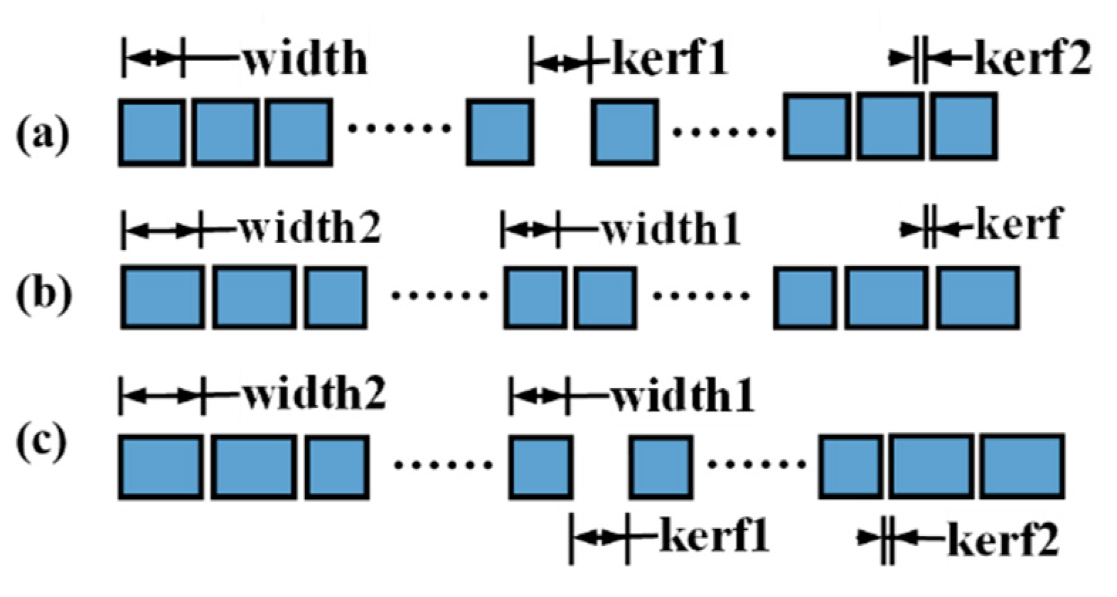
2.1. Transducer Model of MNULA
2.2. Sound Field of Linear Array
2.3. Coherent Plane Wave Compounding Imaging for MNULA
3. Simulation
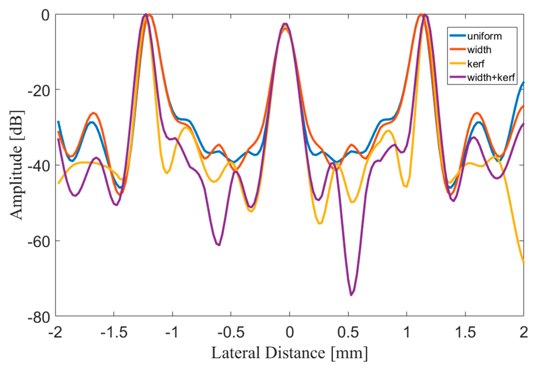
3.1. Sound Field
3.1.1. Settings
3.1.2. Results
3.2. Imaging
3.2.1. Settings
3.2.2. Point Phantom
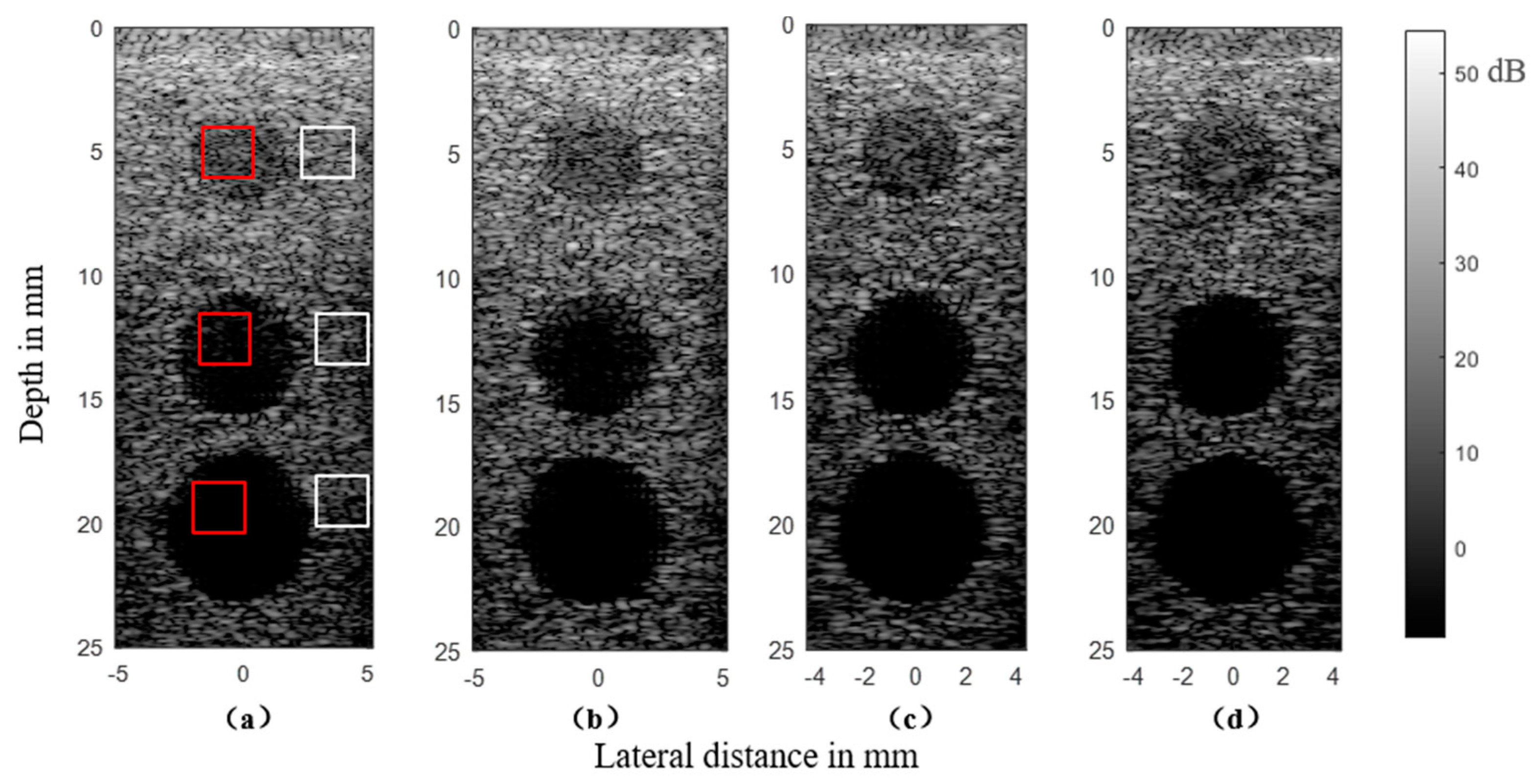
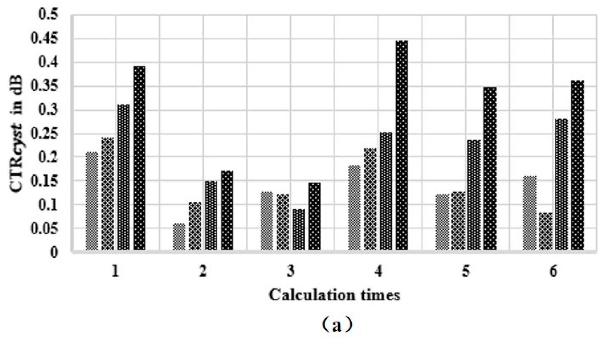
3.2.3. Cyst Phantom
4. Experiment
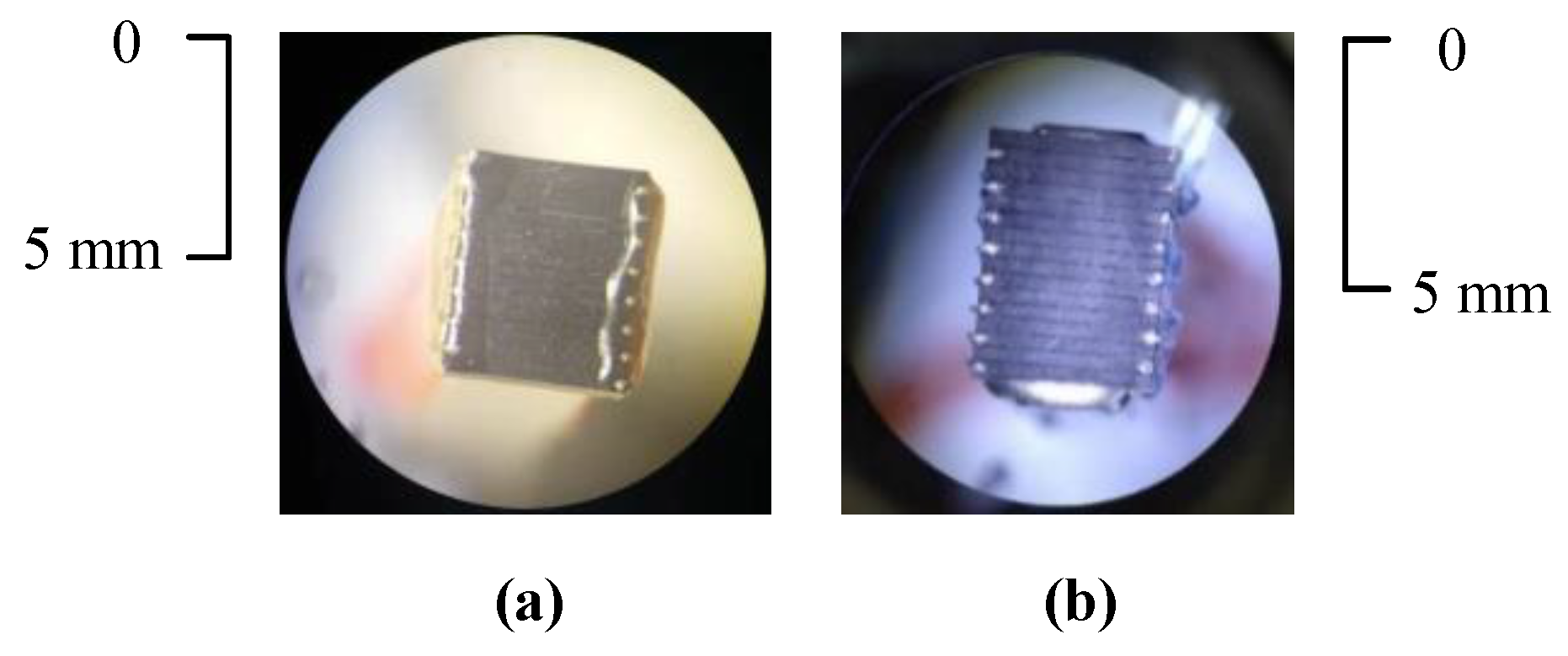
4.1. Transducer Quality Evaluation
4.2. Experimental Setup
4.3. Results and Analysis
5. Discussion
6. Conclusions
Author Contributions
Funding
Institutional Review Board Statement
Informed Consent Statement
Data Availability Statement
Conflicts of Interest
References
- Berson, M.; Roncin, A. Compound scanning with an electrically steered beam. Ultrason. Imaging 1981, 3, 303–308. [Google Scholar] [CrossRef]
- Jespersen, S.K.; Wilhjelm, J.E. Multi-angle compound imaging. Ultrason. Imaging 1998, 20, 81–102. [Google Scholar] [CrossRef] [PubMed]
- Entrekin, R.R.; Porter, B.A. Real-time spatial compound imaging: Application to breast, vascular, and musculoskeletal ultrasound. Semin. Ultrasound CT MRI 2001, 22, 50–64. [Google Scholar] [CrossRef]
- Montaldo, G.; Tanter, M. Coherent Plane-Wave Compounding for Very High Frame Rate Ultrasonography and Transient Elastography. IEEE Trans. Ultrason. Ferroelectr. Freq. Control 2009, 56, 489–506. [Google Scholar] [CrossRef] [PubMed]
- Jensen, J.A.; Svendsen, N.B. Calculation of Pressure Fields from arbitarily Shaped, Apodized, and Ecited Ultrasound Transducers. IEEE Trans. Ultrason. Ferroelectr. Freq. Control 1992, 39, 262–267. [Google Scholar] [CrossRef] [PubMed]
- Tanter, M.; Bercoff, J.; Athanasiou, A.; Deffieux, T.; Gennisson, J.-L.; Montaldo, G.; Muller, M.; Tardivon, A.; Fink, M. Quantitative Assessment of Breast Lesion Viscoelasticity: Initial Clinical Results Using Supersonic Shear Imaging. Ultrasound Med. Biol. 2008, 34, 1373–1386. [Google Scholar] [CrossRef] [PubMed]
- Osmanski, B.; Pernot, M.; Montaldo, G.; Bel, A.; Messas, E.; Tanter, M. Ultrafast Doppler Imaging of Blood Flow Dynamics in the Myocardium. IEEE Trans. Med Imaging 2012, 31, 1661–1668. [Google Scholar] [CrossRef] [PubMed]
- Mickael, T.; Mathias, F. Ultrafast imaging in biomedical ultrasound. IEEE Trans. Ultrason. Ferroelectr. Freq. Control 2014, 61, 102–119. [Google Scholar]
- Duman, D.G.; Alahdab, Y. Usefuelness of Endoscopic Ultrasonography (EUS-E) to Measur Liver Stiffness. Hepatology 2019, 70, 1128–1129. [Google Scholar]
- Lv, H.; Zhu, G.; Zhou, L. Diagnostic value of endoscopic ultrasound elastography for benign and malignant digestive system tumors. Pak. J. Med Sci. 2019, 35, 1461–1465. [Google Scholar] [CrossRef]
- Shiratori, Y.; Ikeya, T.; Fukuda, K. Endoscopic Doppler probe ultrasonography for post-endoscopic submucosal dissection ulcer: New device to show blood flow depth. Dig. Endosc. 2019, 31, 721. [Google Scholar] [CrossRef] [PubMed]
- Gress, F.G.; Hawes, R.H.; Savides, T.J.; Ikenberry, S.O.; Lehman, G.A. Endoscopic ultrasound–guided fine-needle aspiration biopsy using linear array and radial scanning endosonography. Gastrointest. Endosc. 1997, 45, 243–250. [Google Scholar] [CrossRef]
- Shattuck, D.P.; Weinshenker, M.D. Explososcan—A parallerl processing technique for ultrasound imaging with linear phased-arrays. J. Acoust. Soc. Am. 1984, 75, 1273–1282. [Google Scholar] [CrossRef]
- Chen, K.; Lee, B.C.; Thomenius, K.; Khuri-Yakub, B.T.; Lee, H.-S.; Sodini, C.G.; Sodini, C.G. A column-row-parallel ultrasound imaging architecture for 3d plane-wave imaging and Tx 2nd-order harmonic distortion (HD2) reduction. IEEE Int. Ultrason. Symp. 2014, 65, 317–320. [Google Scholar] [CrossRef]
- Yu, C.-C. Sidelobe reduction of asymmetric linear array by spacing perturbation. Electron. Lett. 1997, 33, 730. [Google Scholar] [CrossRef]
- Kumar, B.P.; Branner, G.R. Design of unequally spaced arrays for performance improvement. IEEE Trans. Antennas Propag. 1999, 47, 511–523. [Google Scholar] [CrossRef]
- Unz, H. Linear Arrays with arbitrarily distributed elements. IRE Trans. Antennas Propag. 1960, 8, 222–223. [Google Scholar] [CrossRef]
- Kumar, B.P.; Branner, G.R. Generalized analytical technique for the synthesis of unequally spaced arrays with linear, pla-nar, cylindrical or spherical geometry. IEEE Trans. Antennas Propag. 2005, 53, 621–634. [Google Scholar] [CrossRef]
- Moffet, A. Minimum-redundancy linear arrays. IRE Trans. Antennas Propag. 1968, 16, 172–175. [Google Scholar] [CrossRef]
- Suzuki, K.; Higuchi, K.; Tanigawa, H. A silicon electrostatic ultrasonic transducer. IEEE Trans. Ultrason. Ferroelectr. Freq. Control 1989, 36, 620–627. [Google Scholar] [CrossRef]
- Tang, Y.; Jiao, Y.; Li, Z.; Lv, J.; Yang, C.; Cui, Y. Ultrasound Plane-Wave Imaging Based on Linear Arrays with Variable Inter-element Spacings. In Proceedings of the IEEE International Ultrasonics Symposium, Glasgow, UK, 3–9 October 2019. [Google Scholar]
- Garcia, D.; Tarnec, L.L. Stolt’s f-k migration for plane wave ultrasound imaging. IEEE Trans. Ultrason. Ferroelectr. Freq. Control 2013, 60, 1853–1867. [Google Scholar] [CrossRef] [PubMed]
- Zhao, J.; Wang, Y.; Zeng, X.; Yu, J.; Yiu, B.Y.S.; Yu, A.C.H. Plane wave compounding based on a joint transmitting-receiving adaptive beamformer. IEEE Trans. Ultrason. Ferroelectr. Freq. Control 2015, 62, 1440–1452. [Google Scholar] [CrossRef] [PubMed]
- Jiqi, C.; Jian-Yu, L. Extended high-frame rate imaging method with limited-diffraction beams. IEEE Trans. Ultrason. Ferroelectr. Freq. Control 2006, 53, 880–899. [Google Scholar] [CrossRef] [PubMed]
- Ultrasound Imaging System Performance Assessment. Available online: http://www.aapm.org/meetings/03aM/pdf/9905-9859.pdf (accessed on 8 September 2003).
- Lo, Y.; Lee, S. A study of space-tapered arrays. IRE Trans. Antennas Propag. 2004, 14, 22–30. [Google Scholar] [CrossRef]
- Cen, L.; Ser, W.; Cen, W.; Yu, Z.L. Linear sparse array synthesis via convex optimization. In Proceedings of the 2010 IEEE International Symposium on Circuits and Systems, Pairs, France, 30 May–2 June 2010; pp. 4233–4236. [Google Scholar]
- Lin, C.; Qing, A.; Feng, Q. Synthesis of Unequally Spaced Antenna Arrays by Using Differential Evolution. IEEE Trans. Antennas Propag. 2010, 58, 2553–2561. [Google Scholar] [CrossRef]


| Structural Parameters | Uniform | Nonuniform1 | Nonuniform2 | Nonunifrom3 |
|---|---|---|---|---|
| Kerf1 (μm) | 25 | 25 | 25 | 25 |
| No. of kerf1 | 8 | 8 | 4 | 4 |
| Kerf2 (μm) | — | — | 15 | 15 |
| No. of kerf2 | — | — | 4 | 4 |
| Width1 (μm) | 300 | 300 | 300 | 300 |
| No. of width1 | 8 | 4 | 8 | 4 |
| Width2 (μm) | — | 200 | — | 200 |
| No. of width2 | — | 4 | — | 4 |
| Structural Parameters | MULA | MNULA |
|---|---|---|
| Kerf1 (μm) | 25 | 15 |
| No. of kerf1 | 8 | 8 |
| Kerf2 (μm) | 25 | 25 |
| No. of kerf2 | 8 | 8 |
| Width1 (μm) | 300 | 300 |
| No. of width1 | 8 | 8 |
| Width2 (μm) | 300 | 300 |
| No. of width2 | 8 | 8 |
Publisher’s Note: MDPI stays neutral with regard to jurisdictional claims in published maps and institutional affiliations. |
© 2021 by the authors. Licensee MDPI, Basel, Switzerland. This article is an open access article distributed under the terms and conditions of the Creative Commons Attribution (CC BY) license (http://creativecommons.org/licenses/by/4.0/).
Share and Cite
Tang, Y.; Li, Z.; Cui, Y.; Yang, C.; Lv, J.; Jiao, Y. Micro Non-Uniform Linear Array (MNULA) for Ultrasound Plane Wave Imaging. Sensors 2021, 21, 640. https://doi.org/10.3390/s21020640
Tang Y, Li Z, Cui Y, Yang C, Lv J, Jiao Y. Micro Non-Uniform Linear Array (MNULA) for Ultrasound Plane Wave Imaging. Sensors. 2021; 21(2):640. https://doi.org/10.3390/s21020640
Chicago/Turabian StyleTang, Yujia, Zhangjian Li, Yaoyao Cui, Chen Yang, Jiabing Lv, and Yang Jiao. 2021. "Micro Non-Uniform Linear Array (MNULA) for Ultrasound Plane Wave Imaging" Sensors 21, no. 2: 640. https://doi.org/10.3390/s21020640
APA StyleTang, Y., Li, Z., Cui, Y., Yang, C., Lv, J., & Jiao, Y. (2021). Micro Non-Uniform Linear Array (MNULA) for Ultrasound Plane Wave Imaging. Sensors, 21(2), 640. https://doi.org/10.3390/s21020640