Quantitative Evaluations with 2d Electrical Resistance Tomography in the Low-Conductivity Solutions Using 3d-Printed Phantoms and Sucrose Crystal Agglomerate Assessments


Abstract
1. Introduction
2. ERT Imaging
2.1. Modeling and Simulation Studies in ERT
2.2. Reconstruction Methods
2.3. ERT and Quantitative Spatial Evaluations
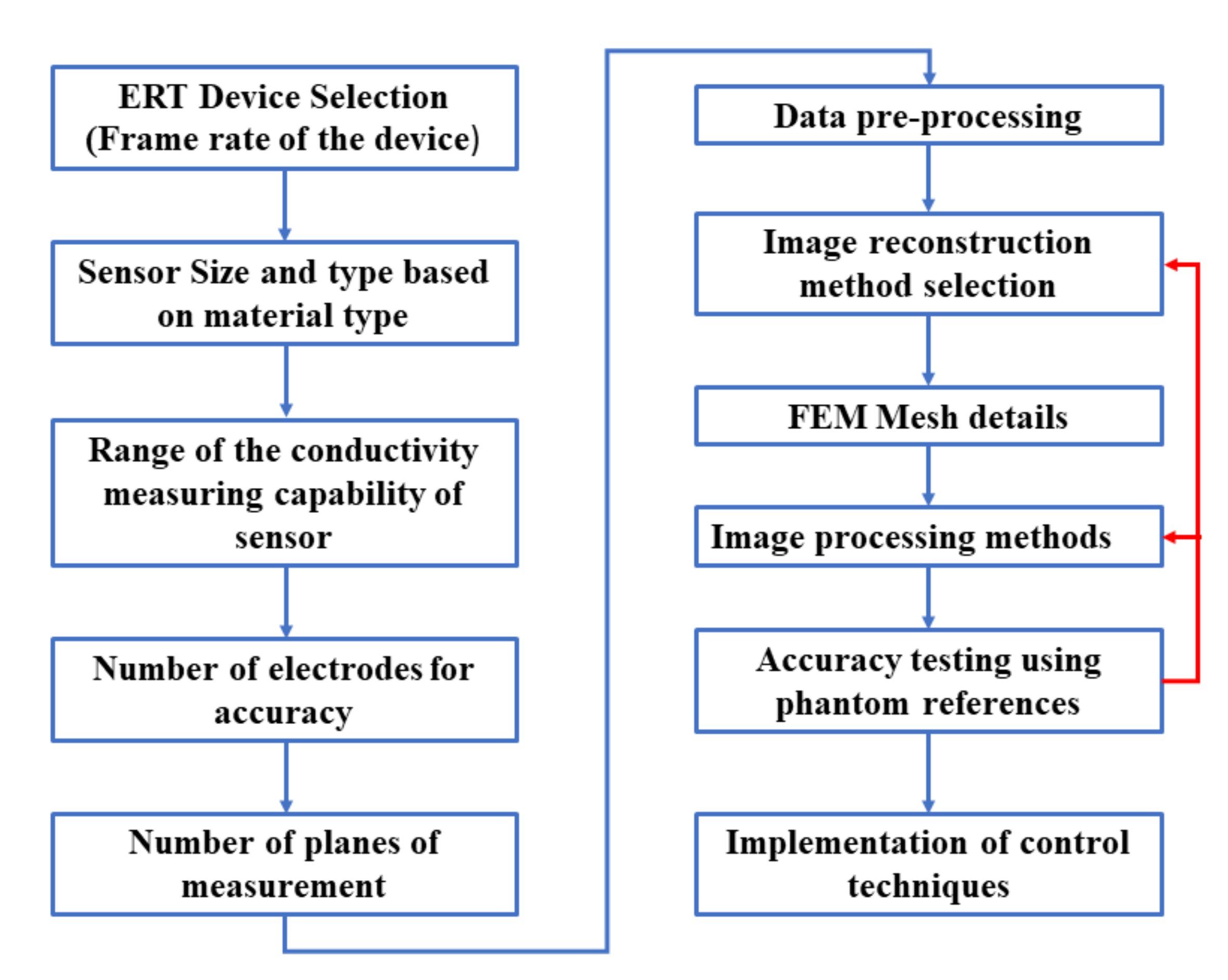
3. Experimental Design
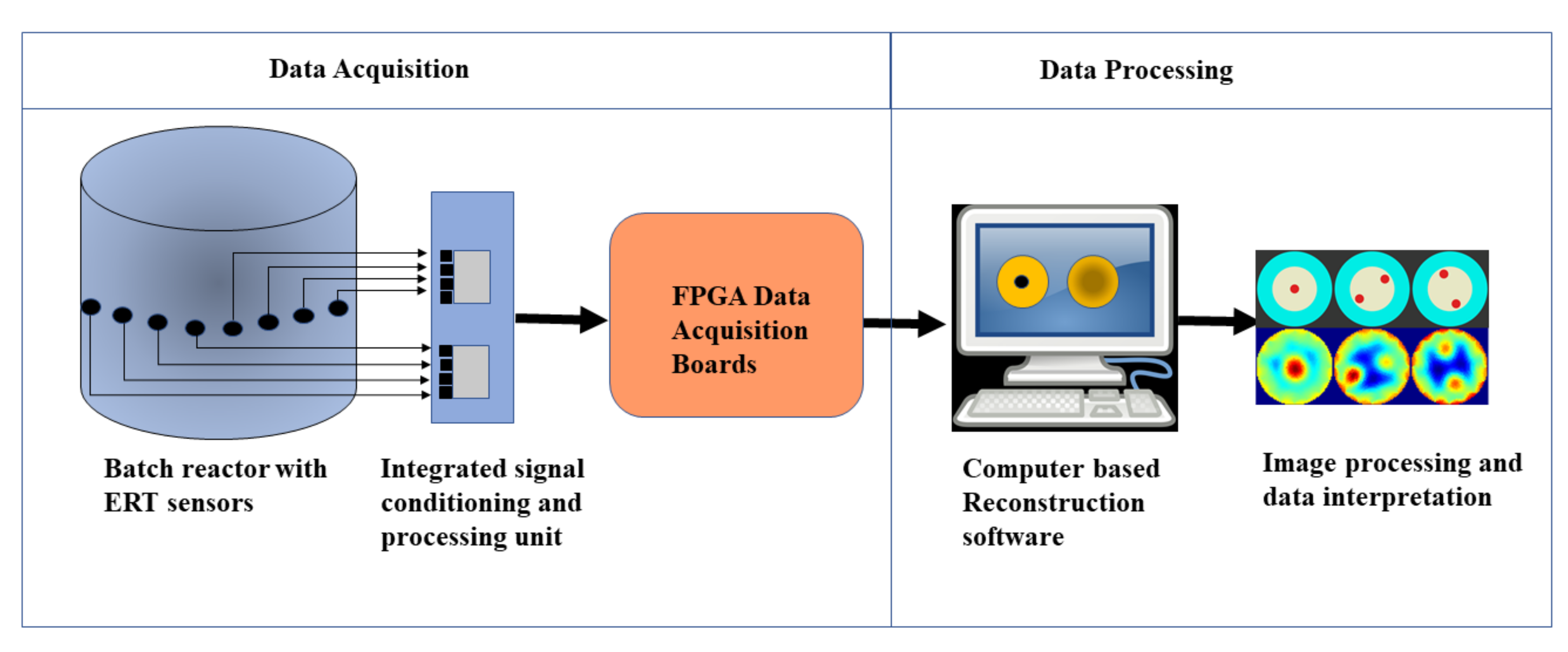
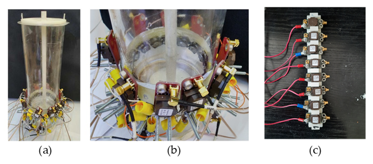
3.1. Experimental Setup and Sensor Design
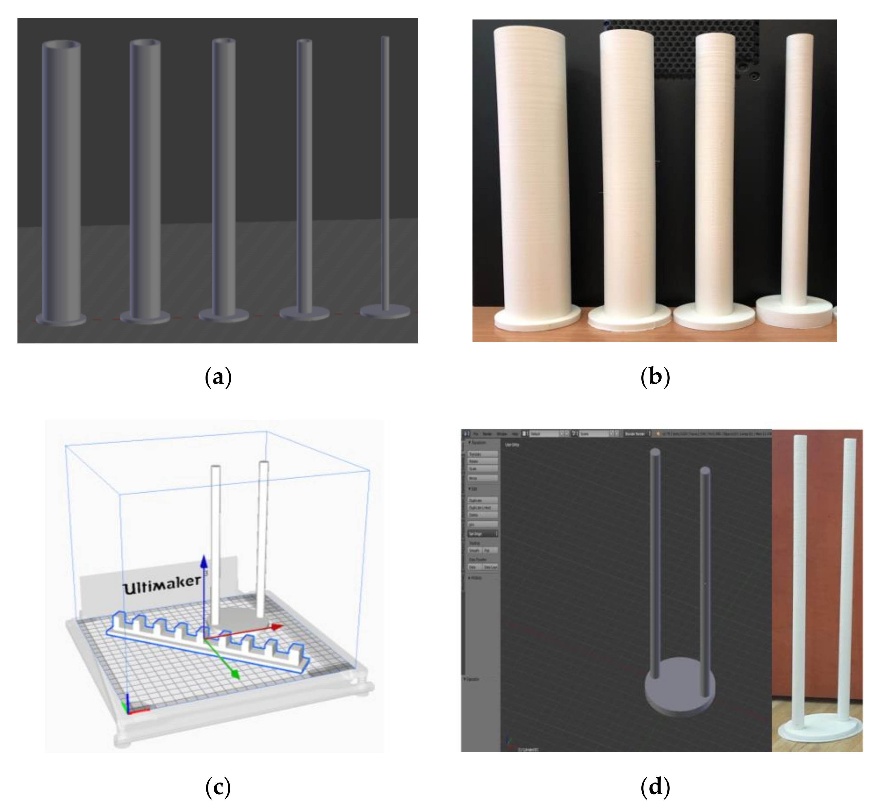
3.2. Phantom Design and 3D Printing
3.3. Sucrose Crystal Agglomerate Assesments, Experimental Progression, and Test Objectives
4. Results
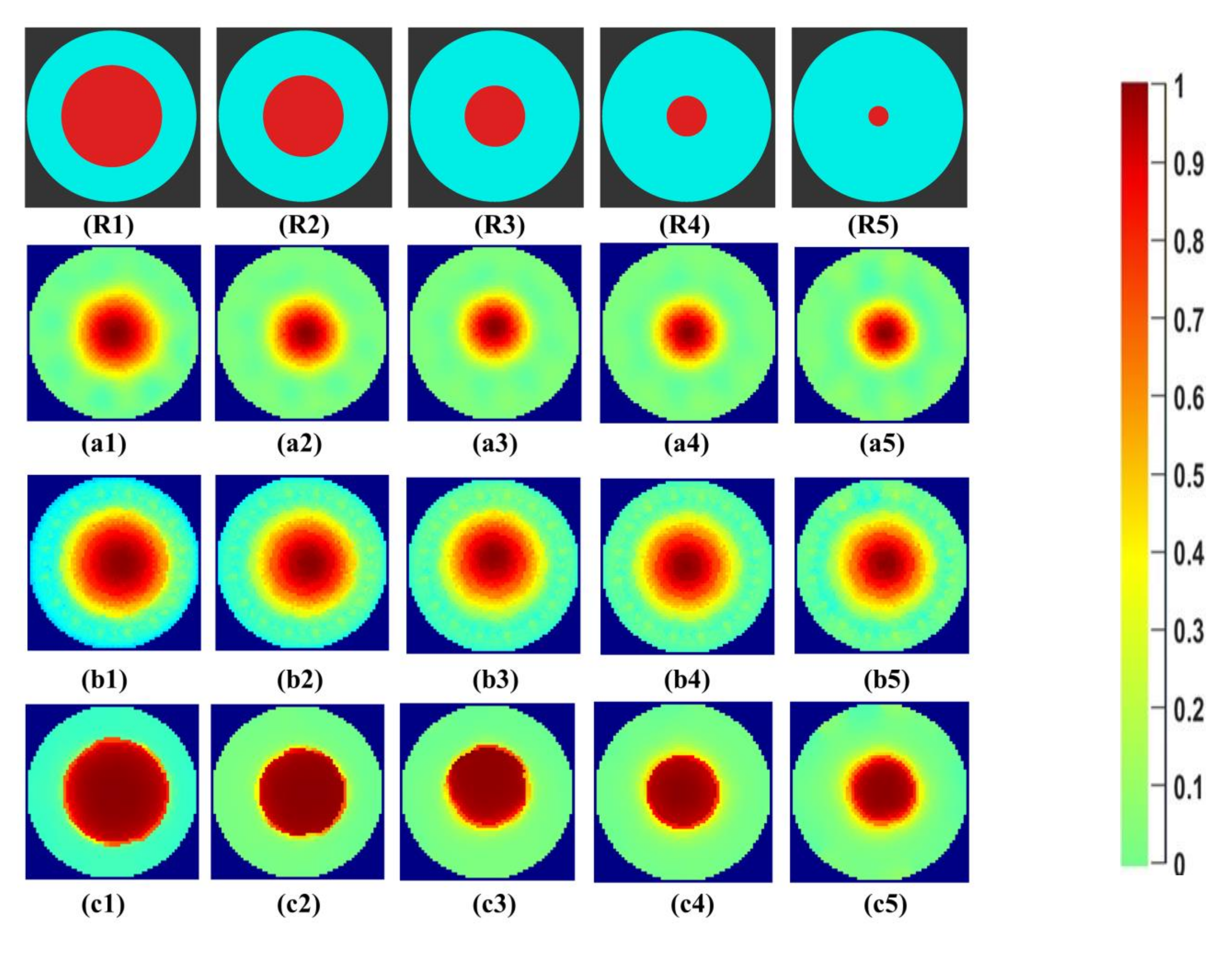
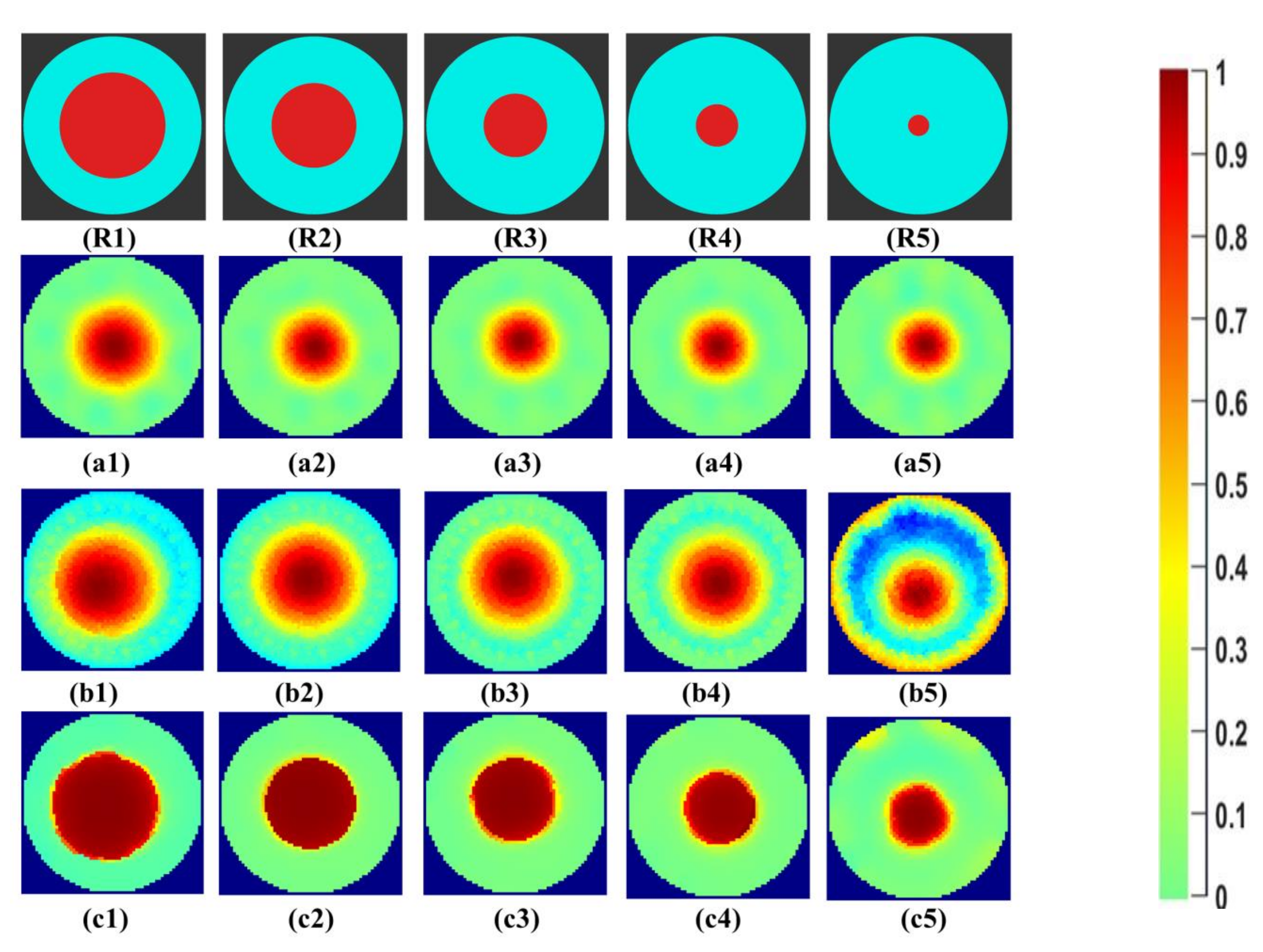
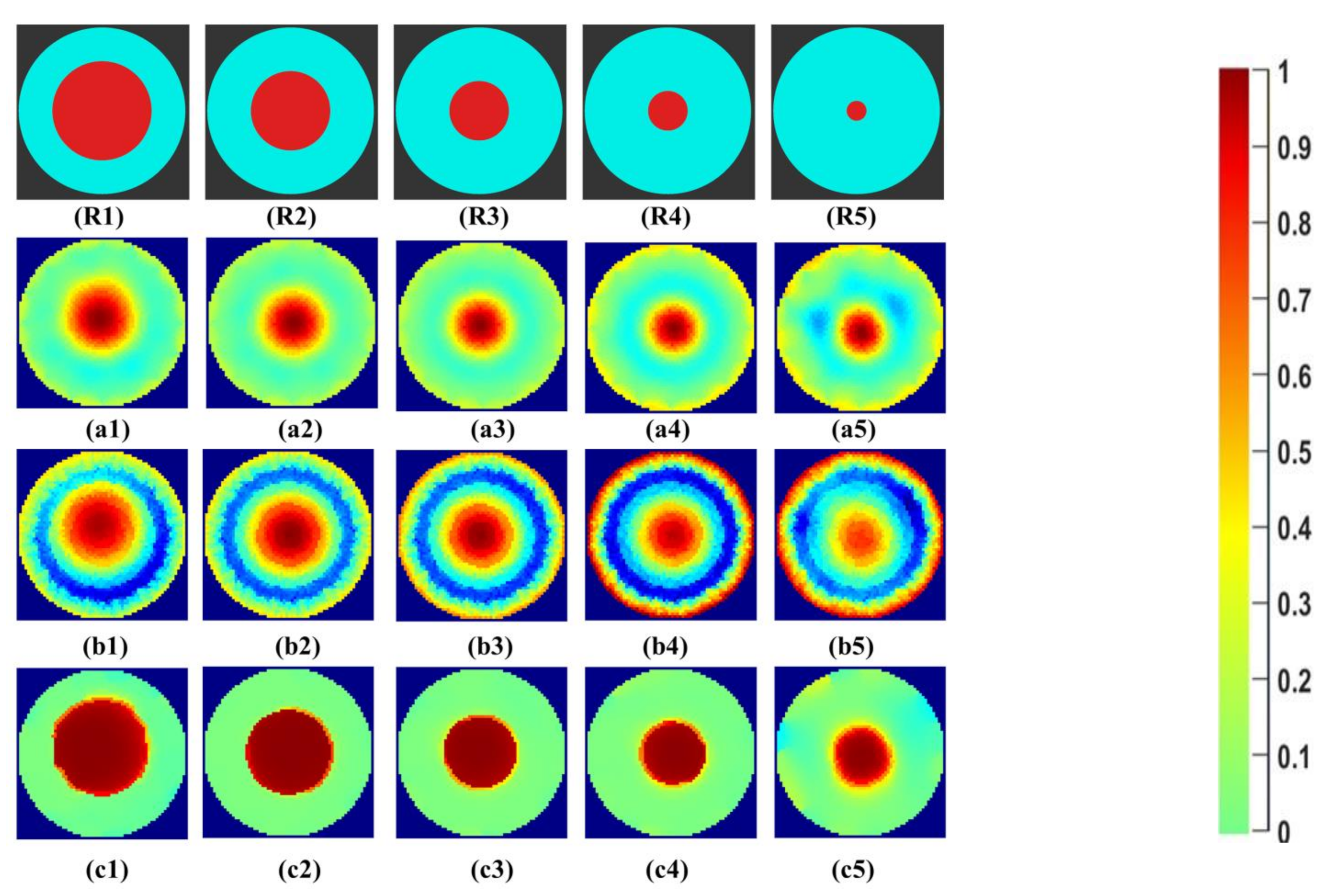
4.1. Differences Due to Reconstruction Methods
4.2. Varying the Iterations in the TV Reconstruction
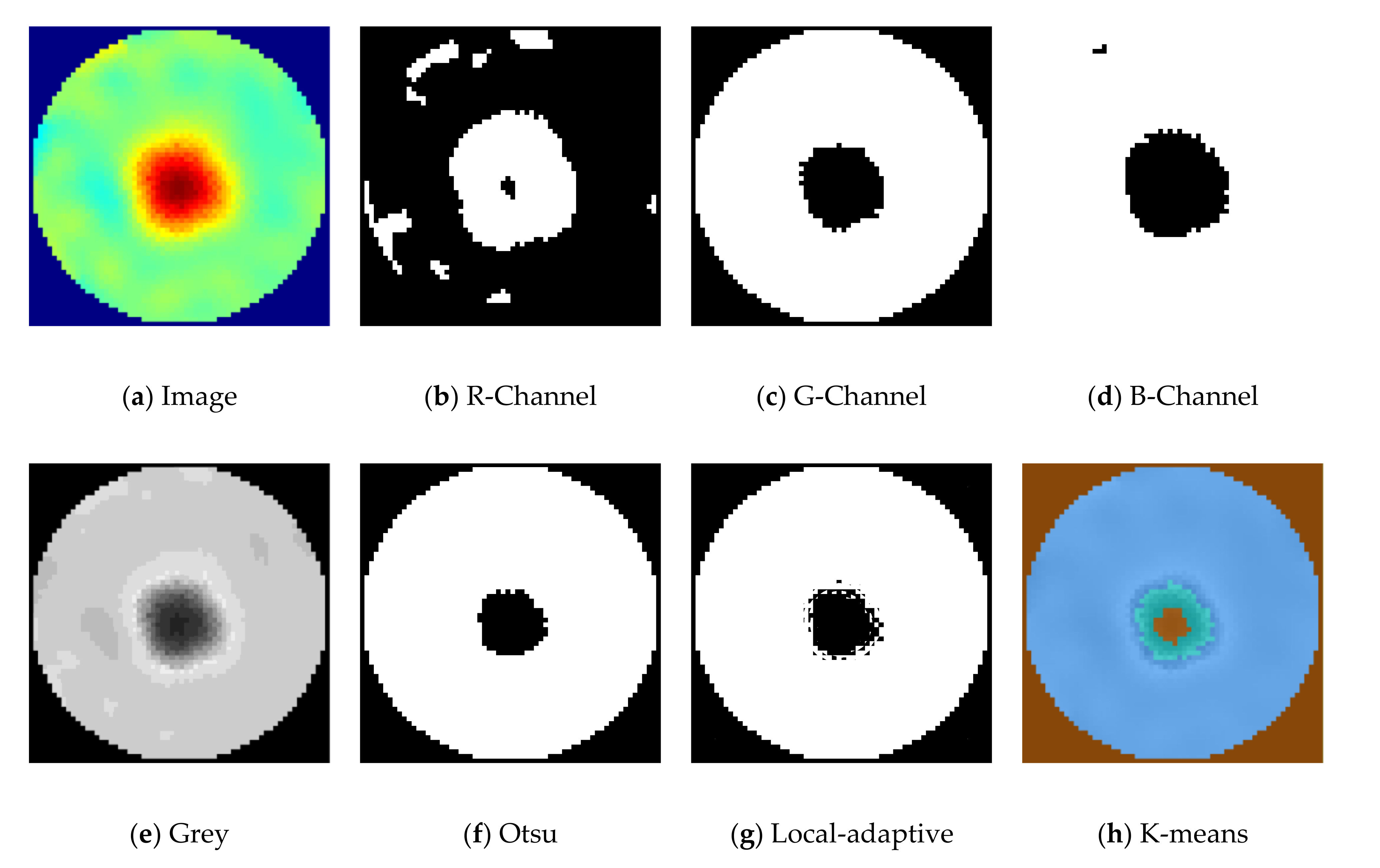
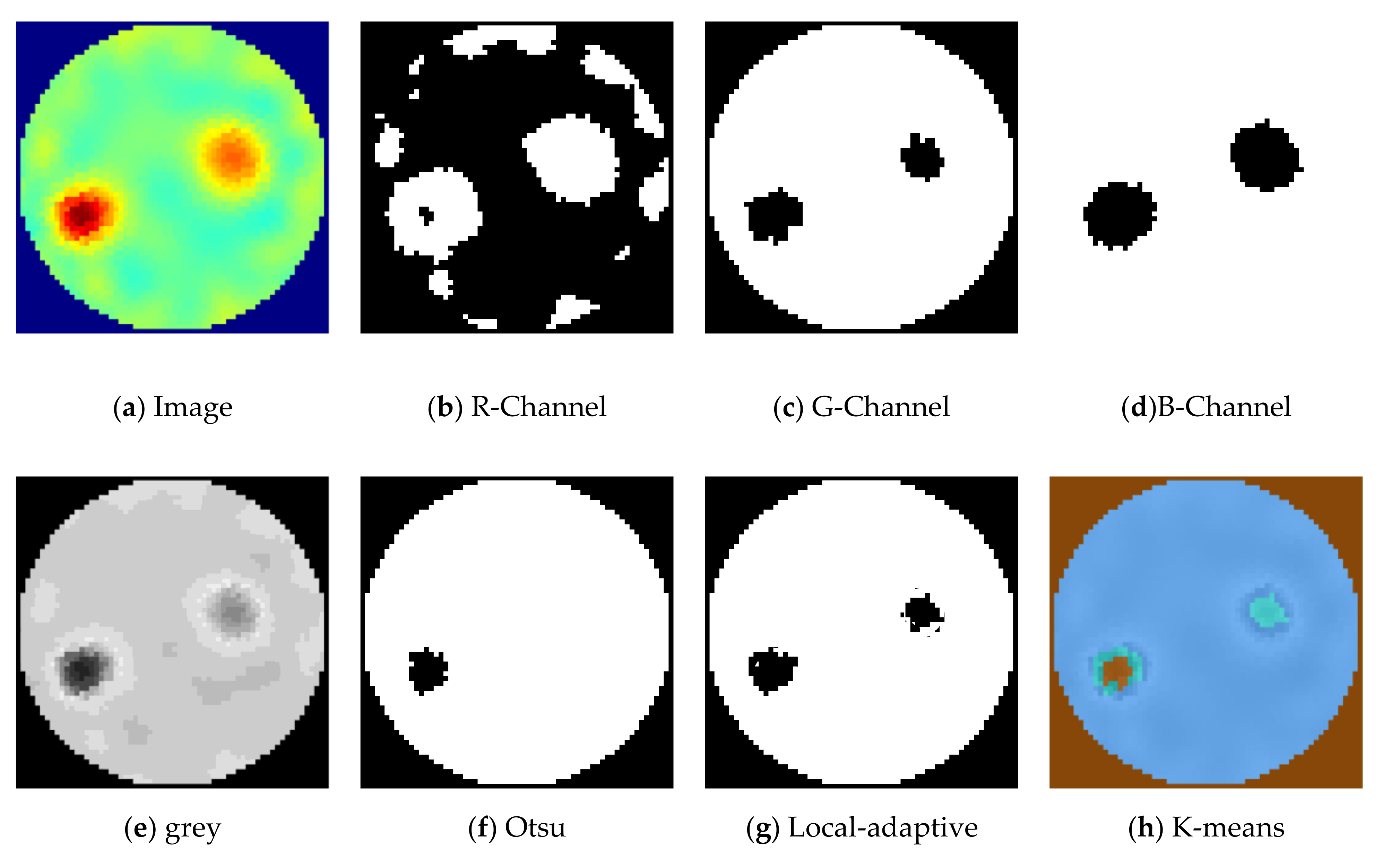
4.3. Analysing Segmentation Methods and Morphological Image Processing
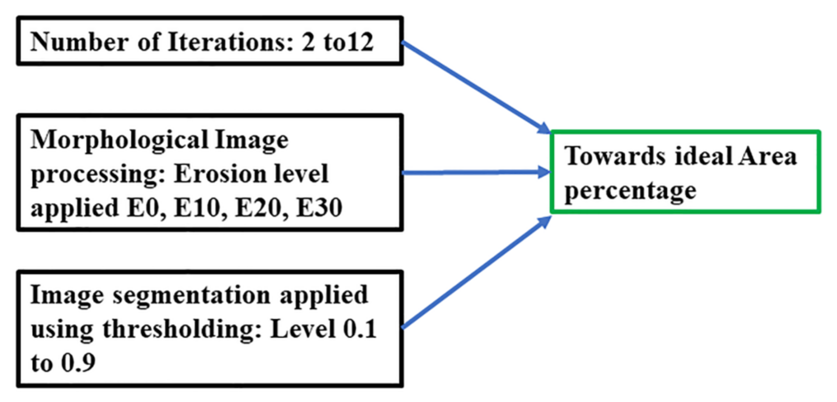
4.4. Towards Quantitative Estimations Using a Combination of Image Processing Methods to Achieve the Expected Area Estimation
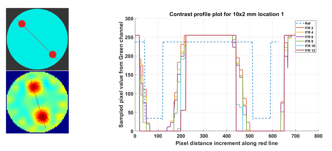
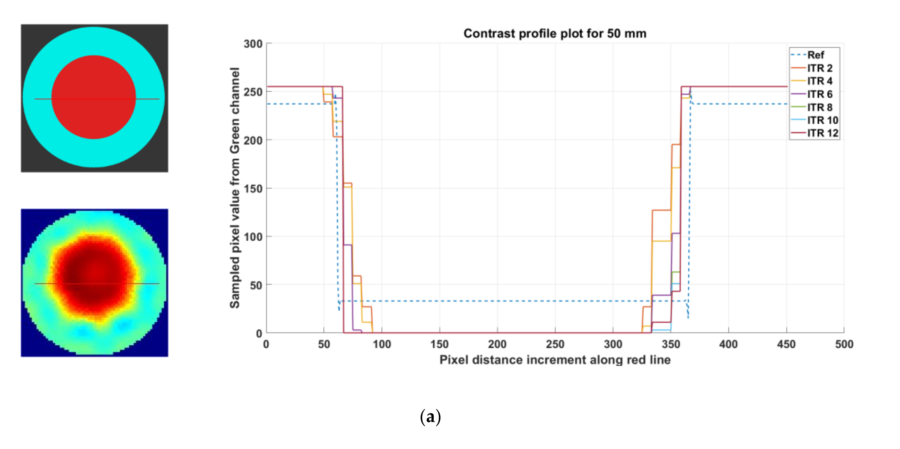
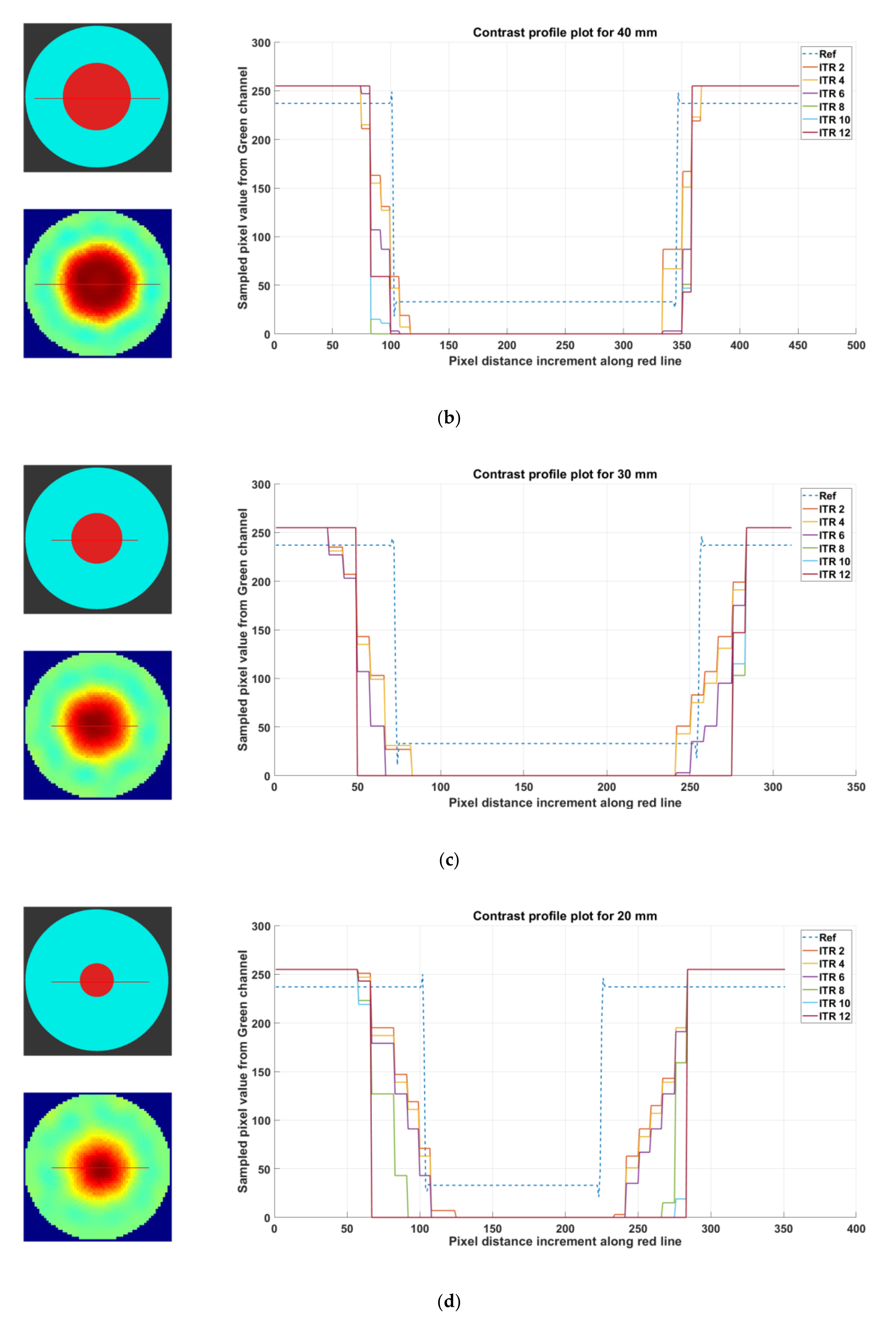
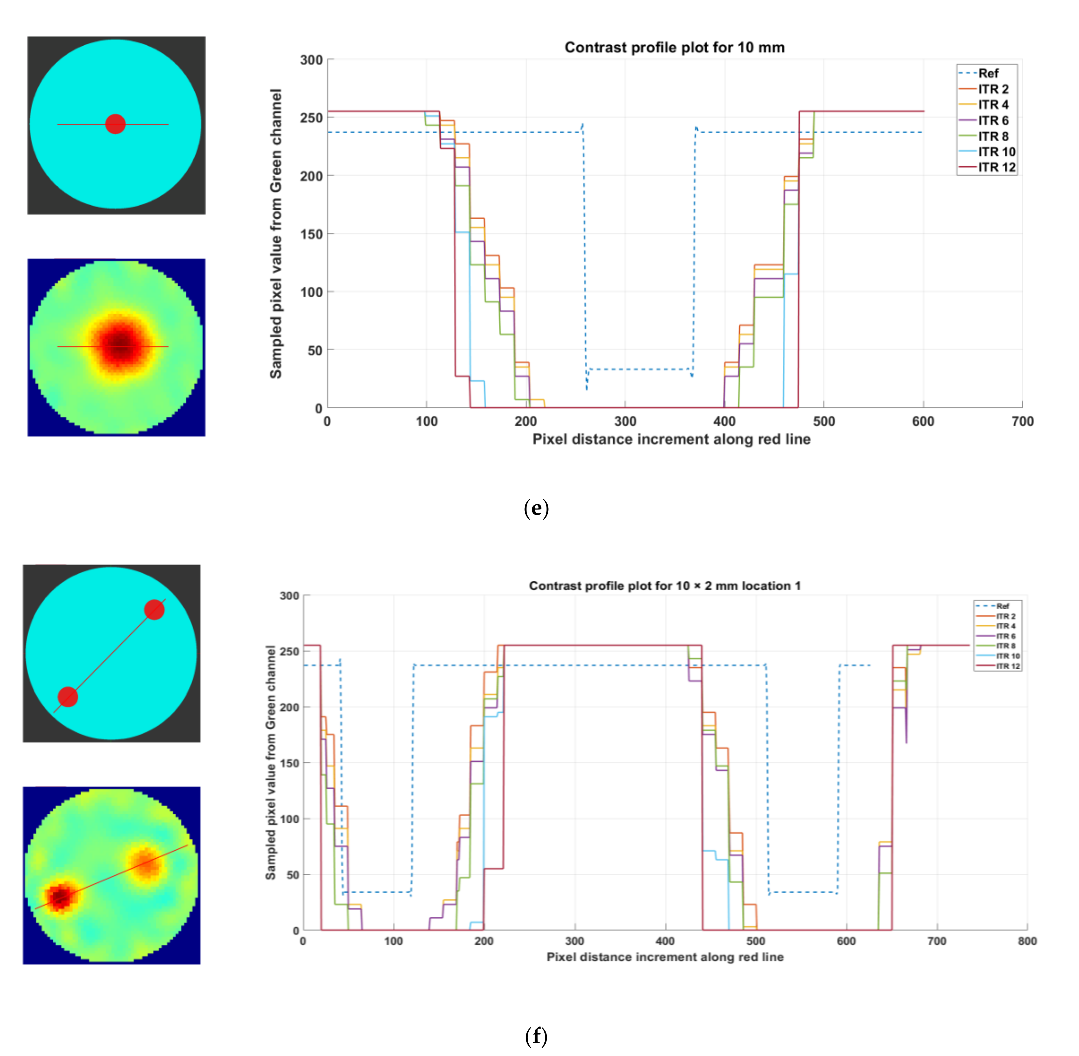
4.4.1. Contrast Profile Assessment at Various Iteration Levels
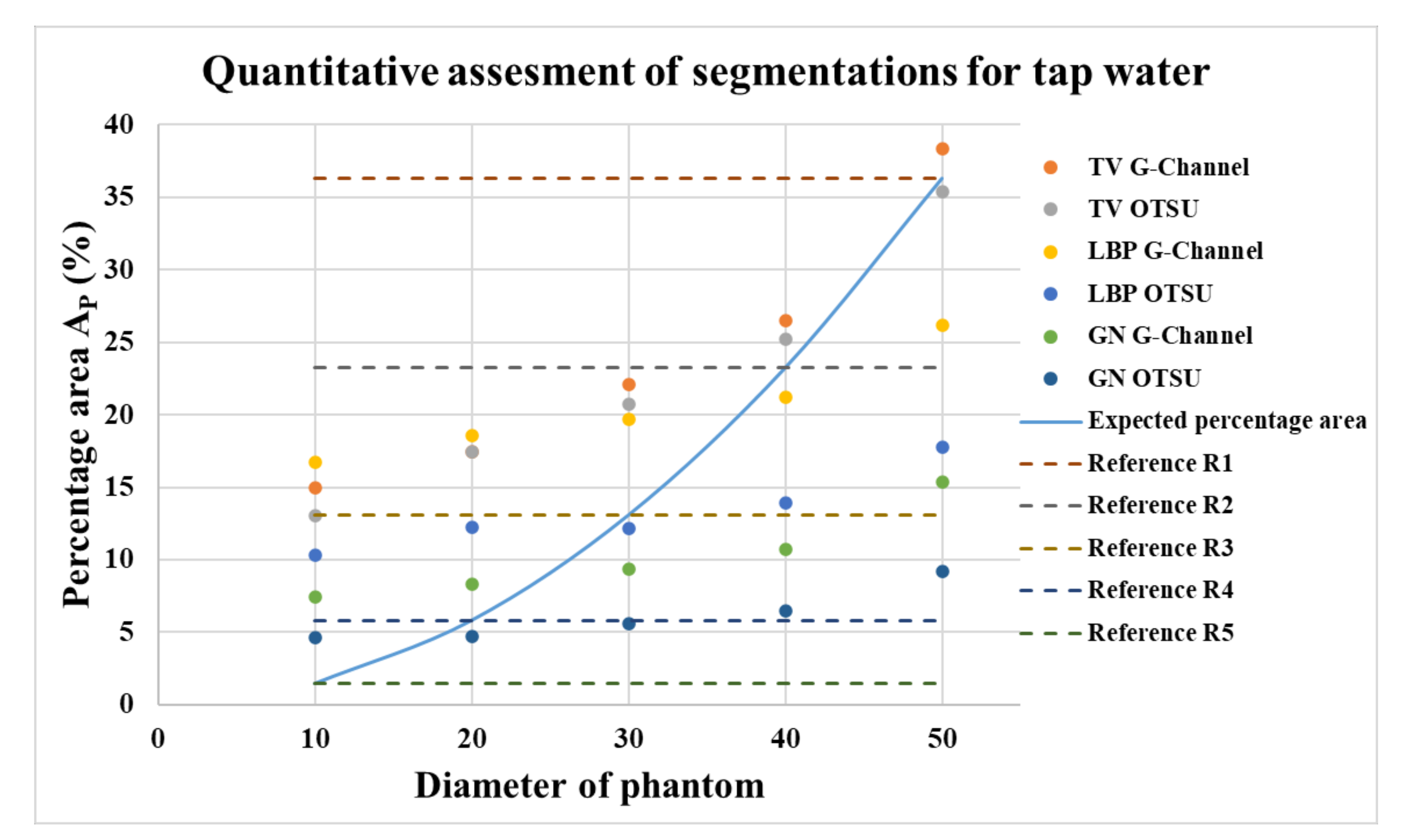
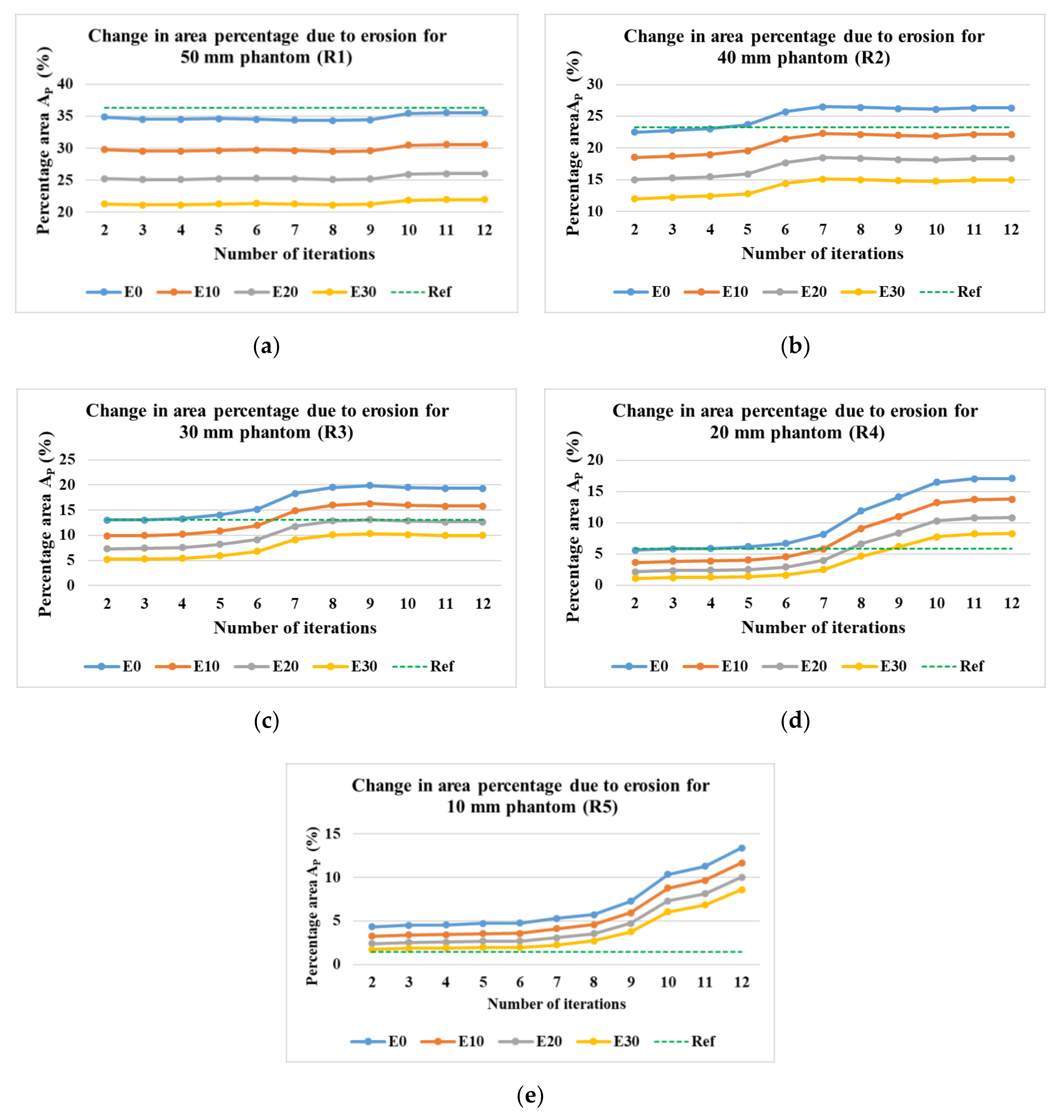
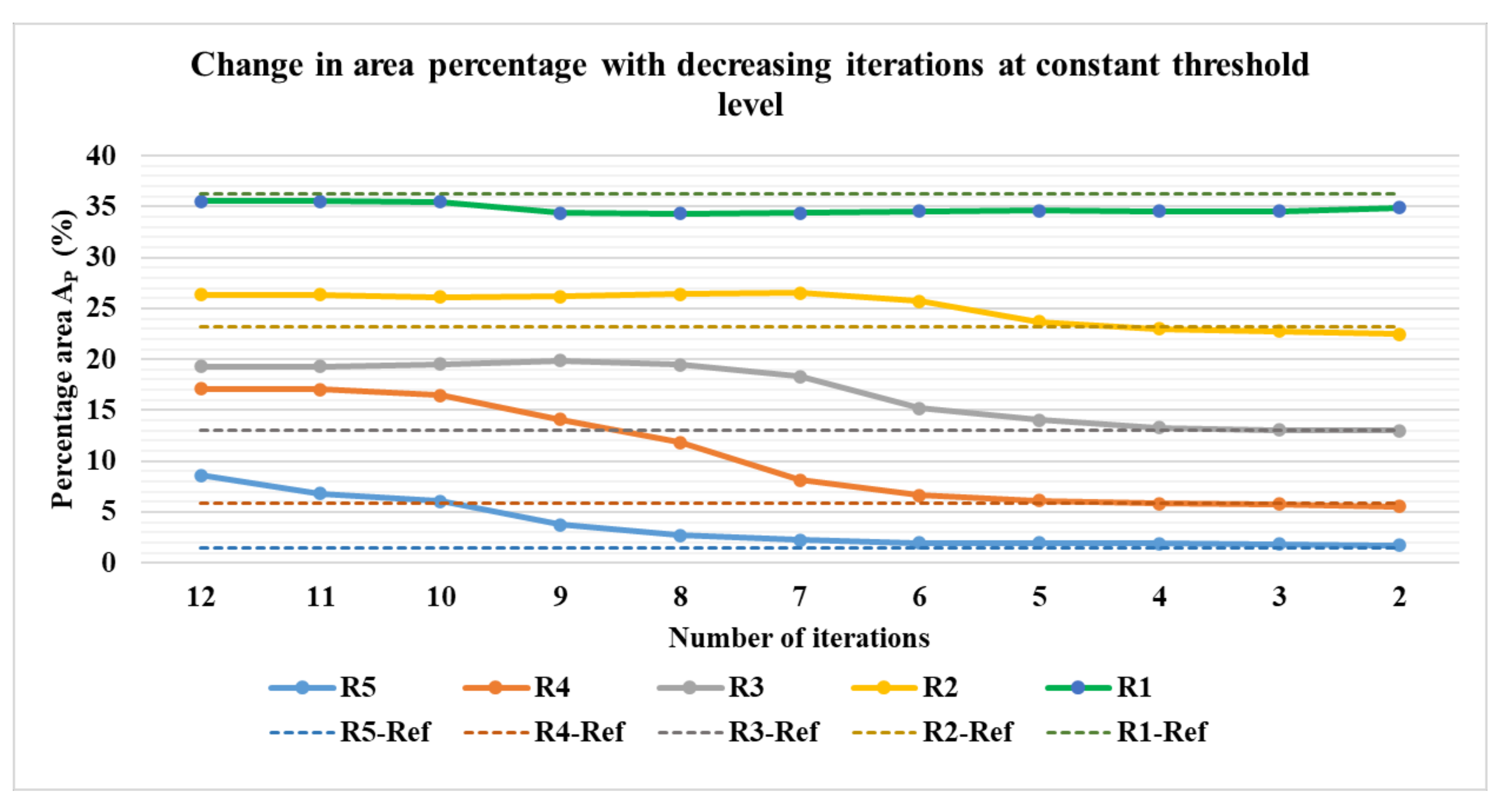
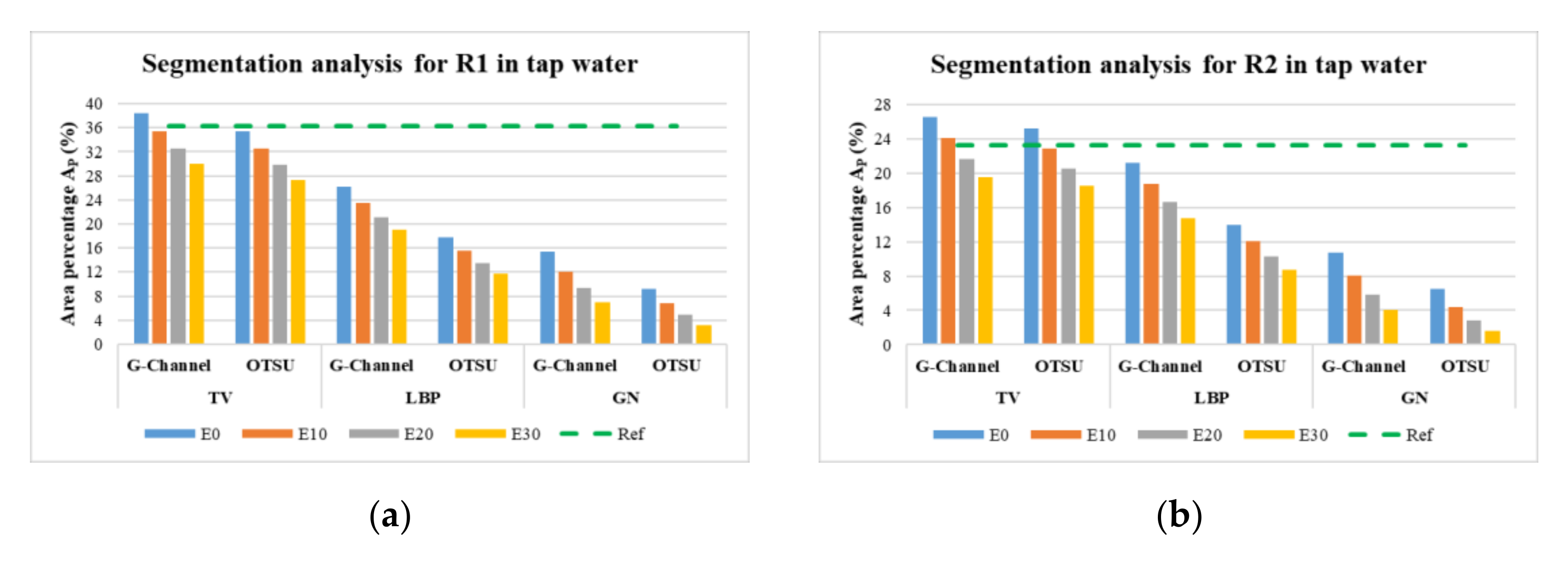
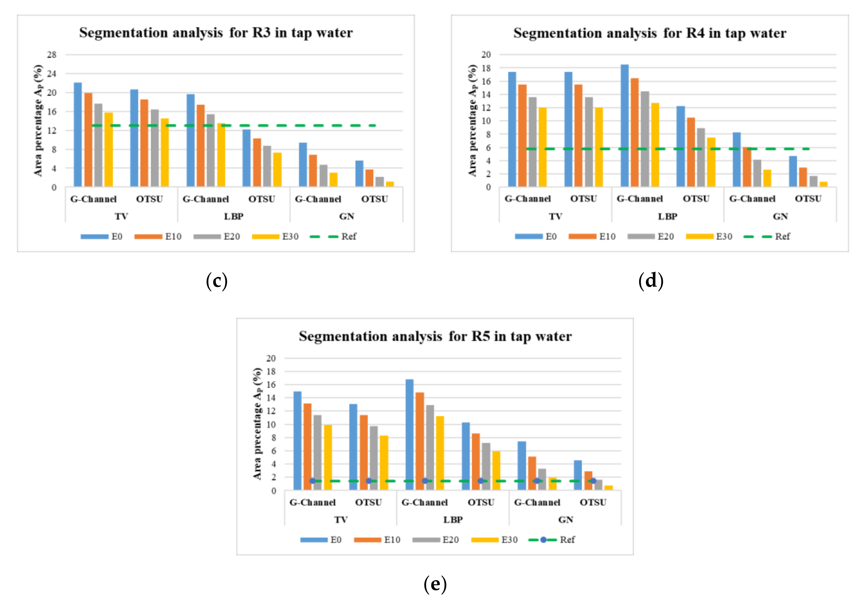
4.4.2. Evaluation of the Area Covered by Phantoms at Various Iterations
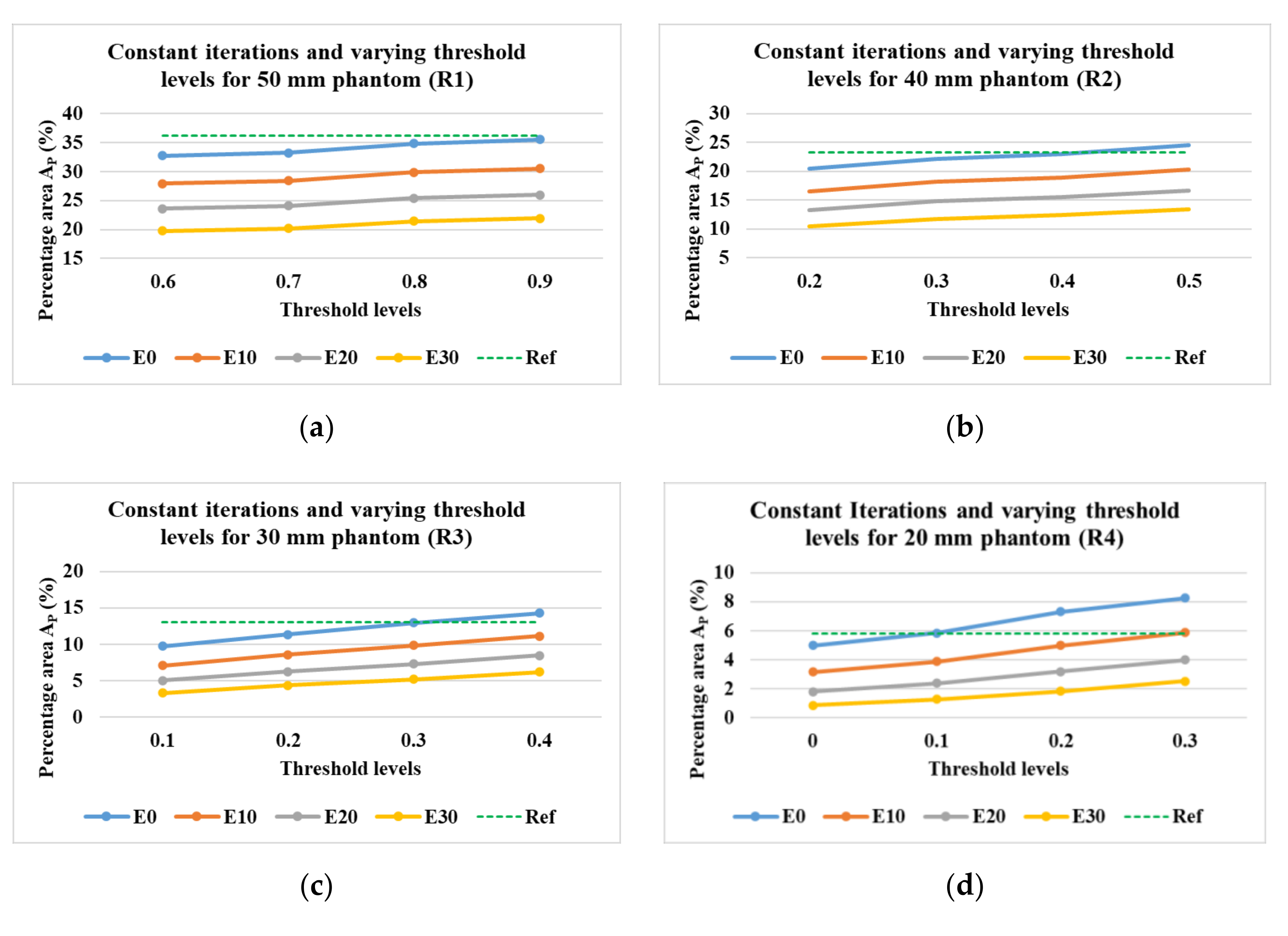
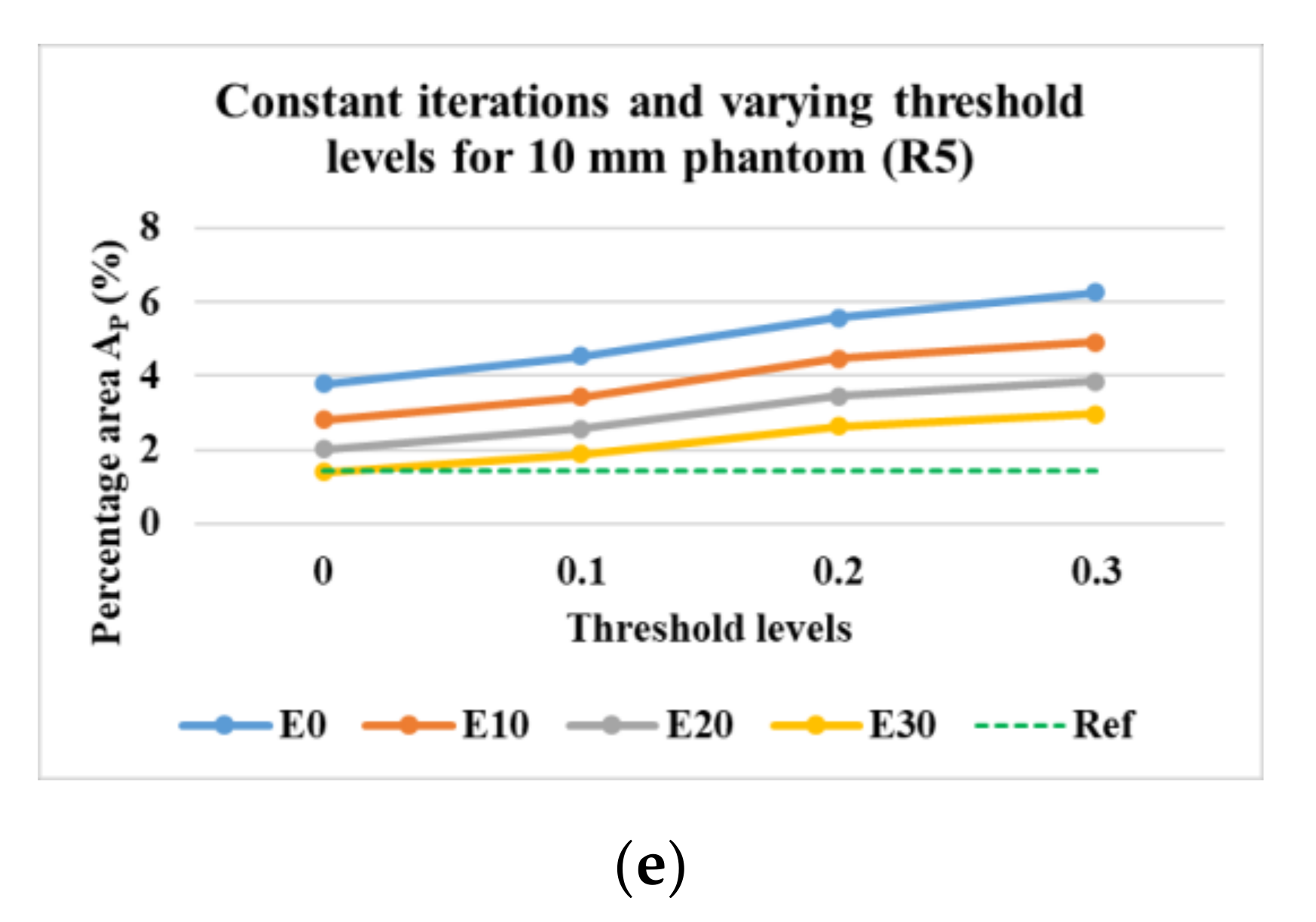
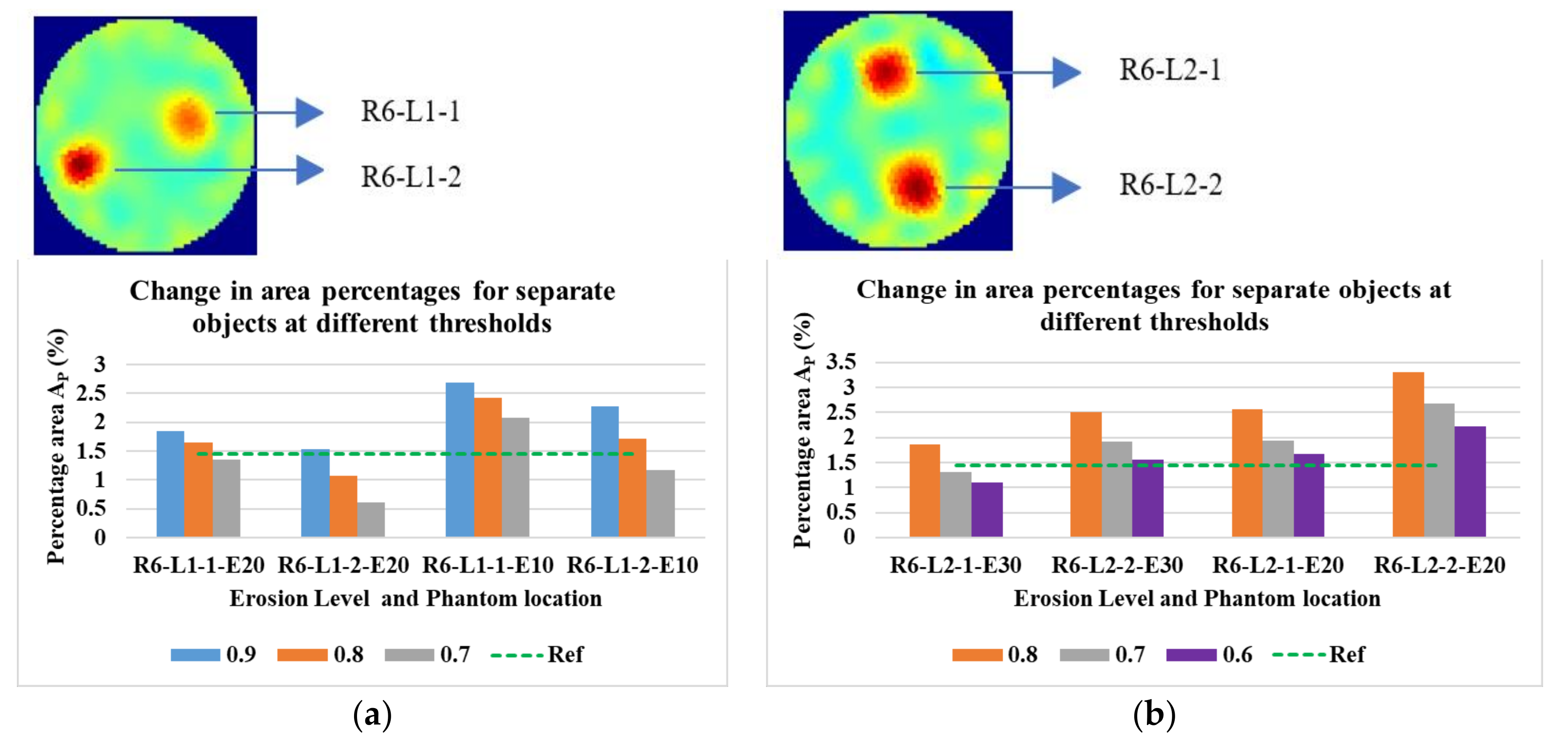
4.4.3. Evaluation of the Area Covered by Phantoms at Various Threshold Levels
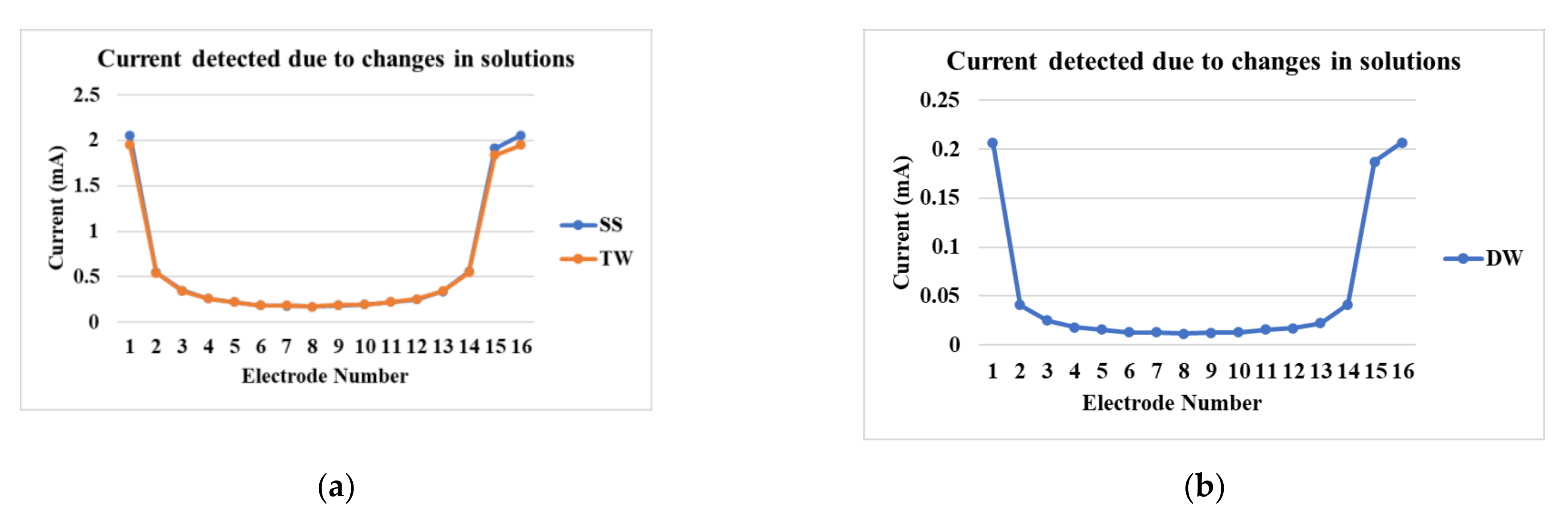
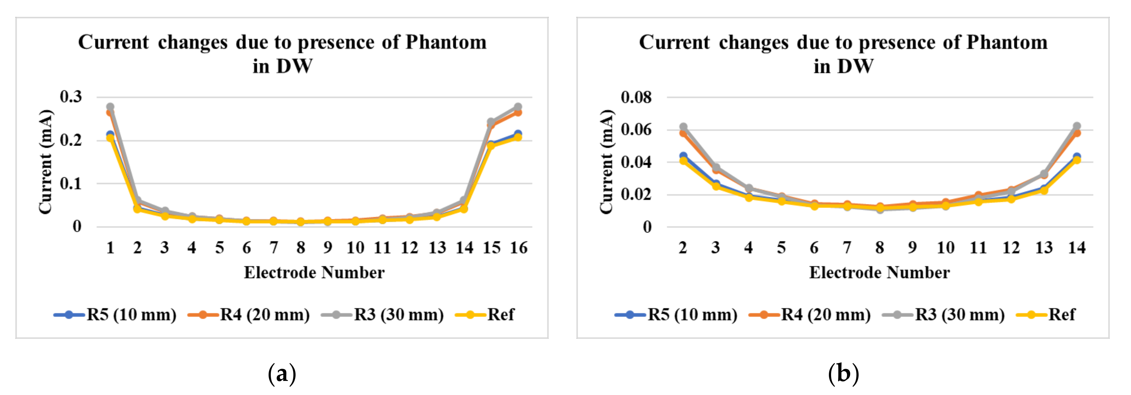
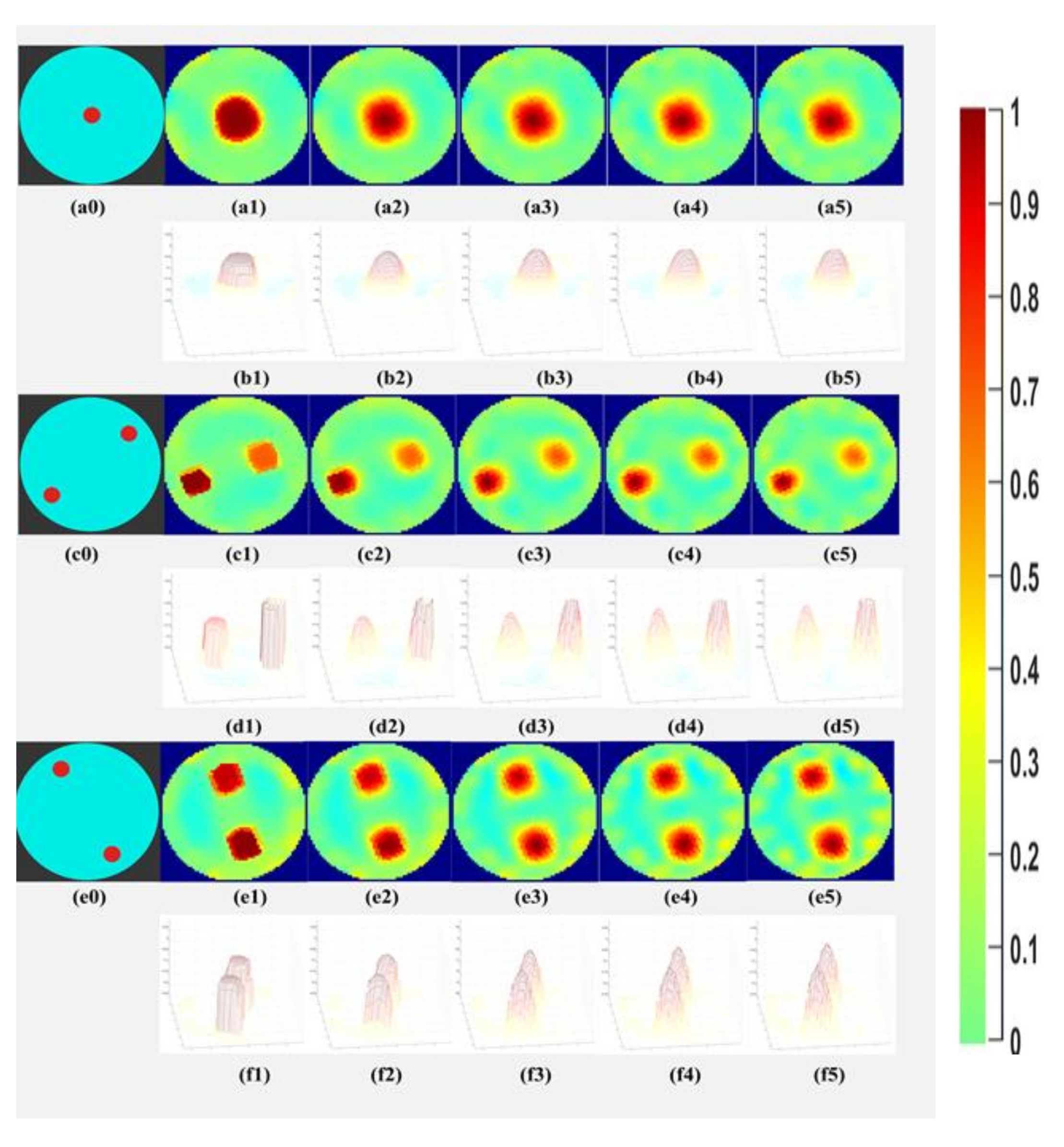
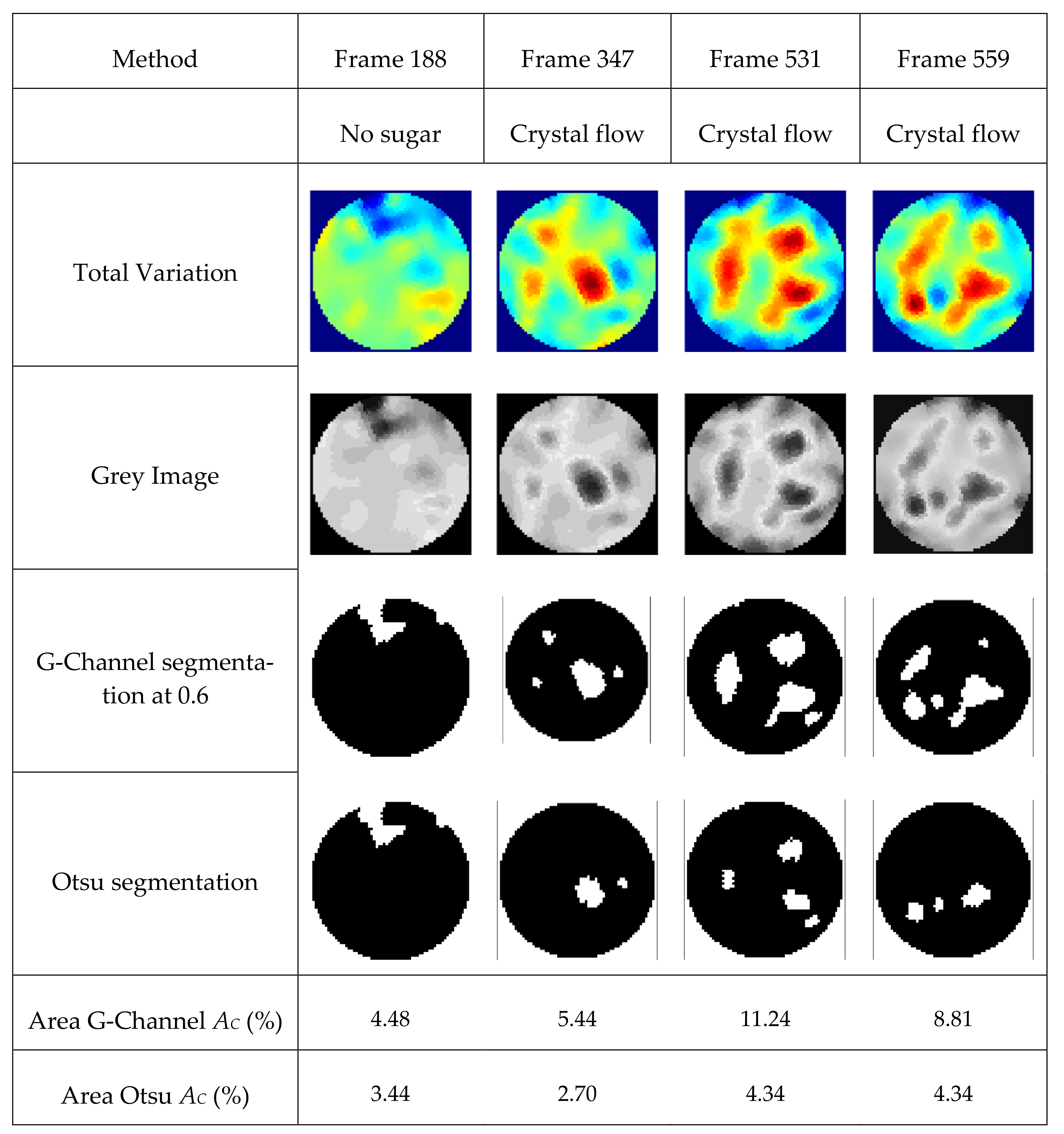
4.5. Experimental Industrial Application in Assessment of Sucrose Crystals in Demineralized Water
5. Conclusions
Author Contributions
Funding
Institutional Review Board Statement
Informed Consent Statement
Data Availability Statement
Acknowledgments
Conflicts of Interest
Appendix A


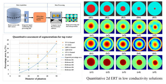
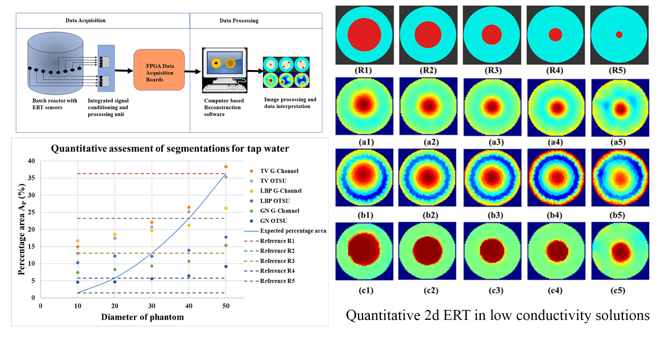
| Corr. PD | Corr. AP | |||||||
|---|---|---|---|---|---|---|---|---|
| Phantom diameter (PD) | 10 | 20 | 30 | 40 | 50 | 0.9811 | ||
| Expected area (AP) | 1.45 | 5.81 | 13.06 | 23.23 | 36.29 | 0.9811 | ||
| TV | G-Channel | 14.99 | 17.44 | 22.10 | 26.48 | 38.38 | 0.9563 | 0.9904 |
| Otsu | 13.06 | 17.44 | 20.69 | 25.23 | 35.39 | 0.9714 | 0.9920 | |
| LBP | G-Channel | 16.76 | 18.53 | 19.66 | 21.21 | 26.16 | 0.9499 | 0.9811 |
| Otsu | 10.29 | 12.22 | 12.13 | 13.90 | 17.76 | 0.9314 | 0.9662 | |
| GN | G-Channel | 7.44 | 8.28 | 9.34 | 10.71 | 15.38 | 0.9255 | 0.9740 |
| Otsu | 4.60 | 4.70 | 5.57 | 6.49 | 9.23 | 0.9196 | 0.9748 | |
| stdevA | 4.63 | 5.69 | 6.84 | 8.18 | 11.59 | |||
| ˄ (%) | 319.14 | 97.95 | 52.33 | 35.20 | 31.95 |
References
- Chakraborty, J.; Sarkar, D.; Singh, A.; Bharti, A.K. Measuring the three-dimensional morphology of crystals using regular reflection of light. Cryst. Growth Des. 2012, 12, 6042–6049. [Google Scholar] [CrossRef]
- Singh, M.R.; Chakraborty, J.; Nere, N.; Tung, H.-H.; Bordawekar, S.; Ramkrishna, D. Image-analysis-based method for 3D crystal morphology measurement and polymorph identification using confocal microscopy. Cryst. Growth Des. 2012, 12, 3735–3748. [Google Scholar] [CrossRef]
- De Sena, R.C.; Soares, M.; Pereira, M.L.O.; da Silva, R.C.D.; do Rosário, F.F.; da Silva, J.F.C. A simple method based on the application of a CCD camera as a sensor to detect low concentrations of barium sulfate in suspension. Sensors 2011, 11, 864–875. [Google Scholar] [CrossRef] [PubMed]
- Abu Bakar, M.; Nagy, Z.; Rielly, C. A combined approach of differential scanning calorimetry and hot-stage microscopy with image analysis in the investigation of sulfathiazole polymorphism. J. Therm. Anal. Calorim. 2010, 99, 609–619. [Google Scholar] [CrossRef][Green Version]
- Soppela, I.; Airaksinen, S.; Hatara, J.; Räikkönen, H.; Antikainen, O.; Yliruusi, J.; Sandler, N. Rapid particle size measurement using 3D surface imaging. Aaps Pharmscitech 2011, 12, 476–484. [Google Scholar] [CrossRef]
- Simone, E.; Saleemi, A.N.; Nagy, Z.K. Raman, UV, NIR, and Mid-IR spectroscopy with focused beam reflectance measurement in monitoring polymorphic transformations. Chem. Eng. Technol. 2014, 37, 1305–1313. [Google Scholar] [CrossRef]
- Verma, S.; Shlichta, P.J. Imaging techniques for mapping solution parameters, growth rate, and surface features during the growth of crystals from solution. Prog. Cryst. Growth Charact. Mater. 2008, 54, 1–120. [Google Scholar] [CrossRef]
- Simon, L.L.; Simone, E.; Oucherif, K.A. Crystallization process monitoring and control using process analytical technology. In Computer Aided Chemical Engineering; Elsevier: Amsterdam, The Netherlands, 2018; Volume 41, pp. 215–242. [Google Scholar]
- De Anda, J.C.; Wang, X.; Lai, X.; Roberts, K.; Jennings, K.; Wilkinson, M.; Watson, D.; Roberts, D. Real-time product morphology monitoring in crystallization using imaging technique. Aiche J. 2005, 51, 1406–1414. [Google Scholar] [CrossRef]
- Sankowski, D.; Sikora, J. Electrical Capacitance Tomography: Theoretical Basis and Applications; Wydawnictwo Książkowe Instytutu Elektrotechniki: Warsaw, Poland, 2010. [Google Scholar]
- Sattar, M.A.; Wrasse, A.D.N.; Morales, R.E.; Pipa, D.R.; Banasiak, R.; Da Silva, M.J.; Babout, L. Multichannel Capacitive Imaging of Gas Vortex in Swirling Two-Phase Flows Using Parametric Reconstruction. IEEE Access 2020, 8, 69557–69565. [Google Scholar] [CrossRef]
- Wajman, R.; Banasiak, R.; Babout, L. On the Use of a Rotatable ECT Sensor to Investigate Dense Phase Flow: A Feasibility Study. Sensors 2020, 20, 4854. [Google Scholar] [CrossRef]
- Kowalska, A.; Banasiak, R.; Romanowski, A.; Sankowski, D. 3D-printed multilayer sensor structure for electrical capacitance tomography. Sensors 2019, 19, 3416. [Google Scholar] [CrossRef]
- Koulountzios, P.; Rymarczyk, T.; Soleimani, M. A Quantitative Ultrasonic Travel-Time Tomography to Investigate Liquid Elaborations in Industrial Processes. Sensors 2019, 19, 5117. [Google Scholar] [CrossRef] [PubMed]
- Rymarczyk, T.; Polakowski, K.; Sikora, J. A new concept of discretisation model for imaging improving in ultrasound transmission tomography. Inform. Autom. Pomiary Gospod. Ochr. Sr. 2019, 9. [Google Scholar] [CrossRef]
- Saad, R.; Nawawi, M.N.M.; Mohamad, E.T. Groundwater detection in alluvium using 2-D electrical resistivity tomography (ERT). Electron. J. Geotech. Eng. 2012, 17, 369–376. [Google Scholar]
- Rymarczyk, T.; Adamkiewicz, P.; Duda, K.; Szumowski, J.; Sikora, J. New electrical tomographic method to determine dampness in historical buildings. Arch. Electr. Eng. 2016, 65, 273–283. [Google Scholar] [CrossRef]
- Kemna, A.; Vanderborght, J.; Kulessa, B.; Vereecken, H. Imaging and characterisation of subsurface solute transport using electrical resistivity tomography (ERT) and equivalent transport models. J. Hydrol. 2002, 267, 125–146. [Google Scholar] [CrossRef]
- Koestel, J.; Kemna, A.; Javaux, M.; Binley, A.; Vereecken, H. Quantitative imaging of solute transport in an unsaturated and undisturbed soil monolith with 3-D ERT and TDR. Water Resour. Res. 2008, 44. [Google Scholar] [CrossRef]
- Woo, E.J.; Hua, P.; Webster, J.G.; Tompkins, W.J. Measuring lung resistivity using electrical impedance tomography. IEEE Trans. Biomed. Eng. 1992, 39, 756–760. [Google Scholar] [CrossRef]
- Sharifi, M.; Young, B. Electrical resistance tomography (ERT) applications to chemical engineering. Chem. Eng. Res. Des. 2013, 91, 1625–1645. [Google Scholar] [CrossRef]
- Rao, G.; Aghajanian, S.; Koiranen, T.; Wajman, R.; Jackowska-Strumiłło, L. Process Monitoring of Antisolvent Based Crystallization in Low Conductivity Solutions Using Electrical Impedance Spectroscopy and 2-D Electrical Resistance Tomography. Appl. Sci. 2020, 10, 3903. [Google Scholar] [CrossRef]
- Yang, Z.; Yan, G. Detection of Impact Damage for Composite Structure by Electrical Impedance Tomography. In ACMSM25; Springer: Berlin/Heidelberg, Germany, 2020; pp. 519–527. [Google Scholar]
- Ghaednia, H.; Owens, C.; Roberts, R.; Tallman, T.N.; Hart, A.J.; Varadarajan, K.M. Interfacial load monitoring and failure detection in total joint replacements via piezoresistive bone cement and electrical impedance tomography. Smart Mater. Struct. 2020, 29, 085039. [Google Scholar] [CrossRef]
- Gao, Z.; Rohani, S.; Gong, J.; Wang, J. Recent developments in the crystallization process: Toward the pharmaceutical industry. Engineering 2017, 3, 343–353. [Google Scholar] [CrossRef]
- Su, Q.; Nagy, Z.K.; Rielly, C.D. Pharmaceutical crystallisation processes from batch to continuous operation using MSMPR stages: Modelling, design, and control. Chem. Eng. Process. Process Intensif. 2015, 89, 41–53. [Google Scholar] [CrossRef]
- Ricard, F.; Brechtelsbauer, C.; Xu, Y.; Lawrence, C.; Thompson, D. Development of an electrical resistance tomography reactor for pharmaceutical processes. Can. J. Chem. Eng. 2005, 83, 11–18. [Google Scholar] [CrossRef]
- Ricard, F.; Brechtelsbauer, C.; Xu, X.; Lawrence, C. Monitoring of multiphase pharmaceutical processes using electrical resistance tomography. Chem. Eng. Res. Des. 2005, 83, 794–805. [Google Scholar] [CrossRef]
- Nagy, Z.; Baker, M.; Pedge, N.; Steele, G. Supersaturation and Direct Nucleation Control of an Industrial Pharmaceutical Crystallisation Process Using a Crystallisation Process Informatics System; Delft Univ. Tech.: Delft, The Netherlands, 2011; pp. 7–9. [Google Scholar]
- Niderla, K.; Rymarczyk, T.; Sikora, J. Manufacturing planning and control system using tomographic sensors. Inform. Control. Econ. Environ. Prot. 2018, 8. [Google Scholar] [CrossRef][Green Version]
- Dodd, R.; Chiou, A.; Broadfoot, R.; Yu, X. Industrial decision support requirements and expectations for a sugar mill crystallisation stage. In Proceedings of the IECON 2011—37th Annual Conference of the IEEE Industrial Electronics Society, Melbourne, VIC, Australia, 7–10 November 2011; pp. 3054–3059. [Google Scholar]
- Sharifi, M.; Young, B. Towards an online milk concentration sensor using ERT: Correlation of conductivity, temperature and composition. J. Food Eng. 2013, 116, 86–96. [Google Scholar] [CrossRef]
- Nagy, Z.K.; Fevotte, G.; Kramer, H.; Simon, L.L. Recent advances in the monitoring, modelling and control of crystallization systems. Chem. Eng. Res. Des. 2013, 91, 1903–1922. [Google Scholar] [CrossRef]
- Lindenberg, C.; Krättli, M.; Cornel, J.; Mazzotti, M.; Brozio, J. Design and optimization of a combined cooling/antisolvent crystallization process. Cryst. Growth Des. 2009, 9, 1124–1136. [Google Scholar] [CrossRef]
- Kovács, I.; Harmat, P.; Sulyok, A.; Radnóczi, G. Investigation of the kinetics of crystallisation of Al/a-Ge bilayer by electrical conductivity measurement. Thin Solid Films 1998, 317, 34–38. [Google Scholar] [CrossRef]
- Rao, G.; Jackowska-Strumiłło, L.; Sattar, M.A.; Wajman, R. Application of the 2D-ERT to evaluate phantom circumscribed regions in various sucrose solution concentrations. In Proceedings of the 2019 International Interdisciplinary PhD Workshop (IIPhDW), Wismar, Germany, 15–17 May 2019. [Google Scholar]
- Carletti, C.; Montante, G.; Westerlund, T.; Paglianti, A. Analysis of solid concentration distribution in dense solid-liquid stirred tanks by electrical resistance tomography. Chem. Eng. Sci. 2014, 119, 53–64. [Google Scholar] [CrossRef]
- Hosseini, S.; Patel, D.; Ein-Mozaffari, F.; Mehrvar, M. Study of solid–liquid mixing in agitated tanks through electrical resistance tomography. Chem. Eng. Sci. 2010, 65, 1374–1384. [Google Scholar] [CrossRef]
- Sardeshpande, M.V.; Kumar, G.; Aditya, T.; Ranade, V.V. Mixing studies in unbaffled stirred tank reactor using electrical resistance tomography. Flow Meas. Instrum. 2016, 47, 110–121. [Google Scholar] [CrossRef]
- Stanley, S.; Mann, R.; Primrose, K. Interrogation of a precipitation reaction by electrical resistance tomography (ERT). Aiche J. 2005, 51, 607–614. [Google Scholar] [CrossRef]
- Boulanger, L. Observations on variations in electrical conductivity of pure demineralized water: Modification (“activation”) of conductivity by low-frequency, low-level alternativing electric fields. Int. J. Biometeorol. 1998, 41, 137–140. [Google Scholar] [CrossRef]
- Dickin, F.; Wang, M. Electrical resistance tomography for process applications. Meas. Sci. Technol. 1996, 7, 247. [Google Scholar] [CrossRef]
- Ma, Y.; Wang, H.; Xu, L.-A.; Jiang, C. Simulation study of the electrode array used in an ERT system. Chem. Eng. Sci. 1997, 52, 2197–2203. [Google Scholar] [CrossRef]
- Yan, P.; Mo, Y. Imaging the complex conductivity distribution in electrical impedance tomography. IFAC Proc. Vol. 2003, 36, 73–76. [Google Scholar] [CrossRef]
- Mann, R.; Williams, R.A.; Dyakowski, T.; Dickin, F.; Edwards, R. Development of mixing models using electrical resistance tomography. Chem. Eng. Sci. 1997, 52, 2073–2085. [Google Scholar] [CrossRef]
- Fransolet, E.; Crine, M.; L’Homme, G.; Toye, D.; Marchot, P. Electrical resistance tomography sensor simulations: Comparison with experiments. Meas. Sci. Technol. 2002, 13, 1239. [Google Scholar] [CrossRef]
- Korteland, S.-A.; Heimovaara, T. Quantitative inverse modelling of a cylindrical object in the laboratory using ERT: An error analysis. J. Appl. Geophys. 2015, 114, 101–115. [Google Scholar] [CrossRef]
- Xiao, L.; Xue, Q.; Wang, H. Finite element mesh optimisation for improvement of the sensitivity matrix in electrical resistance tomography. IET Sci. Meas. Technol. 2015, 9, 792–799. [Google Scholar] [CrossRef]
- Wajman, R.; Banasiak, R. Tunnel-based method of sensitivity matrix calculation for 3D-ECT imaging. Sens. Rev. 2014, 34, 273–283. [Google Scholar] [CrossRef]
- Kim, B.S.; Khambampati, A.K.; Kim, S.; Kim, K.Y. Image reconstruction with an adaptive threshold technique in electrical resistance tomography. Meas. Sci. Technol. 2011, 22, 104009. [Google Scholar] [CrossRef]
- Vauhkonen, M.; Lionheart, W.R.; Heikkinen, L.M.; Vauhkonen, P.J.; Kaipio, J.P. A MATLAB package for the EIDORS project to reconstruct two-dimensional EIT images. Physiol. Meas. 2001, 22, 107. [Google Scholar] [CrossRef] [PubMed]
- Adler, A.; Lionheart, W.R. Uses and abuses of EIDORS: An extensible software base for EIT. Physiol. Meas. 2006, 27, S25. [Google Scholar] [CrossRef] [PubMed]
- Polydorides, N.; Lionheart, W.R.B. A Matlab toolkit for three-dimensional electrical impedance tomography: A contribution to the Electrical Impedance and Diffuse Optical Reconstruction Software project. Meas. Sci. Technol. 2002, 13, 1871. [Google Scholar] [CrossRef]
- Kim, B.S.; Khambampati, A.K.; Jang, Y.J.; Kim, K.Y.; Kim, S. Image reconstruction using voltage–current system in electrical impedance tomography. Nucl. Eng. Des. 2014, 278, 134–140. [Google Scholar] [CrossRef]
- Groetsch, C.W.; Groetsch, C. Inverse Problems in the Mathematical Sciences; Springer: Berlin/Heidelberg, Germany, 1993; Volume 52. [Google Scholar]
- Vaukonen, M. Electrical Impedance Tomography and Prior Information. Ph.D. Thesis, University of Kuopio, Kuopio, Finland, 1997. [Google Scholar]
- Kim, B.S.; Kim, S.; Kim, K.Y. Image reconstruction with prior information in electrical resistance tomography. J. Ikee 2014, 18, 8–18. [Google Scholar] [CrossRef]
- ChuanLei, W.; ShiHong, Y. New selection methods of regularization parameter for electrical resistance tomography image reconstruction. In Proceedings of the 2016 IEEE International Instrumentation and Measurement Technology Conference Proceedings, Taipei, Taiwan, 23–26 May 2016; pp. 1–5. [Google Scholar]
- Borsic, A.; Graham, B.M.; Adler, A.; Lionheart, W.R. Total variation regularization in electrical impedance tomography. Available online: http://eprints.maths.manchester.ac.uk/813/1/TVReglnEITpreprint.pdf (accessed on 1 October 2020).
- Ferrucci, M.; Leach, R.K.; Giusca, C.; Carmignato, S.; Dewulf, W. Towards geometrical calibration of x-ray computed tomography systems—a review. Meas. Sci. Technol. 2015, 26, 092003. [Google Scholar] [CrossRef]
- Choi, C.T.M.; Sun, S.-H. Method for Improving Imaging Resolution of Electrical Impedance Tomography. U.S. Patent No 9,962,105, 8 May 2018. [Google Scholar]
- Cui, Z.; Wang, Q.; Xue, Q.; Fan, W.; Zhang, L.; Cao, Z.; Sun, B.; Wang, H.; Yang, W. A review on image reconstruction algorithms for electrical capacitance/resistance tomography. Sens. Rev. 2016, 36, 429–445. [Google Scholar] [CrossRef]
- Tamburrino, A.; Ventre, S.; Rubinacci, G. Reconstruction techniques for electrical resistance tomography. IEEE Trans. Magn. 2000, 36, 1132–1135. [Google Scholar]
- Yorkey, T.J.; Webster, J.G.; Tompkins, W.J. Comparing reconstruction algorithms for electrical impedance tomography. IEEE Trans. Biomed. Eng. 1987, BME-34, 843–852. [Google Scholar] [CrossRef]
- Wilkinson, A.; Randall, E.; Long, T.; Collins, A. The design of an ERT system for 3D data acquisition and a quantitative evaluation of its performance. Meas. Sci. Technol. 2006, 17, 2088. [Google Scholar] [CrossRef]
- Majchrowicz, M.; Kapusta, P.; Jackowska-Strumiłło, L.; Banasiak, R.; Sankowski, D. Multi-GPU, Multi-Node Algorithms for Acceleration of Image Reconstruction in 3D Electrical Capacitance Tomography in Heterogeneous Distributed System. Sensors 2020, 20, 391. [Google Scholar] [CrossRef] [PubMed]
- Wang, B.; Huang, Z.; Li, H. Design of high-speed ECT and ERT system. In Proceedings of the Journal of Physics: Conference Series, Naha, Okinawa, Japan, 15–17 December 2008; IOP Publishing: Bristol, UK, 2009; Volume 147, p. 012035. [Google Scholar]
- Feng, D.; Cong, X.; Zhang, Z.; Shangjie, R. Design of parallel electrical resistance tomography system for measuring multiphase flow. Chin. J. Chem. Eng. 2012, 20, 368–379. [Google Scholar]
- Garbaa, H.; Jackowska-Strumiłło, L.; Grudzień, K.; Romanowski, A. Application of electrical capacitance tomography and artificial neural networks to rapid estimation of cylindrical shape parameters of industrial flow structure. Arch. Electr. Eng. 2016, 65, 657–669. [Google Scholar] [CrossRef]
- Bera, T.K.; Biswas, S.K.; Rajan, K.; Nagaraju, J. Projection Error Propagation-based regularization (PEPR) method for resistivity reconstruction in electrical impedance tomography (EIT). Measurement 2014, 49, 329–350. [Google Scholar] [CrossRef]
- Li, S.; Wang, H.; Zhang, L.; Fan, W. Image reconstruction of electrical resistance tomography based on image fusion. In Proceedings of the 2011 IEEE International Instrumentation and Measurement Technology Conference, Binjiang, China, 10–12 May 2011; pp. 1–5. [Google Scholar]
- Giguère, R.; Fradette, L.; Mignon, D.; Tanguy, P.A. ERT algorithms for quantitative concentration measurement of multiphase flows. Chem. Eng. J. 2008, 141, 305–317. [Google Scholar] [CrossRef]
- Kim, B.S.; Khambampati, A.K.; Kim, S.; Kim, K.Y. Improving spatial resolution of ERT images using adaptive mesh grouping technique. Flow Meas. Instrum. 2013, 31, 19–24. [Google Scholar] [CrossRef]
- Yue, S.; Wu, T.; Pan, J.; Wang, H. Fuzzy clustering based ET image fusion. Inf. Fusion 2013, 14, 487–497. [Google Scholar] [CrossRef]
- Yuling, W.; Meng, W.; Yan, Y.; Shulan, G. A method to recognize the contaminated area using K-means in ERT contaminated site surveys. In Proceedings of the 2018 IEEE International Conference on Information and Automation (ICIA), Wuyishan, China, 11–13 August 2018; pp. 1587–1591. [Google Scholar]
- Hampel, U.; Wondrak, T.; Bieberle, M.; Lecrivain, G.; Schubert, M.; Eckert, K.; Reinecke, S. Smart Tomographic Sensors for Advanced Industrial Process Control TOMOCON. Chem. Ing. Tech. 2018, 90, 1238–1239. [Google Scholar] [CrossRef]
- Jackson, R.F.; Silsbee, C.G. Saturation Relations in Mixtures of Sucrose, Dextrose, and Levulose; US Government Printing Office: Washington, DC, USA, 1924.
- Mathlouthi, M.; Reiser, P. Sucrose: Properties and Applications; Springer Science & Business Media: Berlin/Heidelberg, Germany, 1995. [Google Scholar]


| Experimental Variable | Count | |
|---|---|---|
| 1 | Number of solutions with varied conductivities | 3 |
| 2 | Number of phantoms | 6 |
| 3 | Number of reconstruction methods compared | 3 |
| 4 | Number of segmentation methods | 4 |
| 5 | Number of electrodes | 16 |
| 6 | Number of planes | 1 |
| 7 | Minimum accuracy tested | 1.5% of the beaker area |
| 8 | Location of object | Central and incremental, separability |
| Object | Measured Values mm | |
|---|---|---|
| 1 | Batch reactor’s inner diameter | 83 |
| 2 | Electrode tail diameter | 5 |
| 3 | Electrode head diameter | 12 |
| Phantom | Measured Values mm | Expected Percentage Area of the Phantom Region (AP) % | |
|---|---|---|---|
| 1 | Phantom R1 | 50 ± 0.1 | 36.28 |
| 2 | Phantom R2 | 40 ± 0.1 | 23.22 |
| 3 | Phantom R3 | 30 ± 0.1 | 13.06 |
| 4 | Phantom R4 | 20 ± 0.1 | 5.8 |
| 5 | Phantom R5 | 10 ± 0.1 | 1.45 |
| 6 | Phantom R6 | 2 × 10 ± 0.1 | 1.45 and 1.45 |
| 5 | Diameter of the base of phantoms | 50 | |
| 7 | Distance between centers of phantom R6 | 40 |
Publisher’s Note: MDPI stays neutral with regard to jurisdictional claims in published maps and institutional affiliations. |
© 2021 by the authors. Licensee MDPI, Basel, Switzerland. This article is an open access article distributed under the terms and conditions of the Creative Commons Attribution (CC BY) license (http://creativecommons.org/licenses/by/4.0/).
Share and Cite
Rao, G.; Sattar, M.A.; Wajman, R.; Jackowska-Strumiłło, L. Quantitative Evaluations with 2d Electrical Resistance Tomography in the Low-Conductivity Solutions Using 3d-Printed Phantoms and Sucrose Crystal Agglomerate Assessments. Sensors 2021, 21, 564. https://doi.org/10.3390/s21020564
Rao G, Sattar MA, Wajman R, Jackowska-Strumiłło L. Quantitative Evaluations with 2d Electrical Resistance Tomography in the Low-Conductivity Solutions Using 3d-Printed Phantoms and Sucrose Crystal Agglomerate Assessments. Sensors. 2021; 21(2):564. https://doi.org/10.3390/s21020564
Chicago/Turabian StyleRao, Guruprasad, Muhammad Awais Sattar, Radosław Wajman, and Lidia Jackowska-Strumiłło. 2021. "Quantitative Evaluations with 2d Electrical Resistance Tomography in the Low-Conductivity Solutions Using 3d-Printed Phantoms and Sucrose Crystal Agglomerate Assessments" Sensors 21, no. 2: 564. https://doi.org/10.3390/s21020564
APA StyleRao, G., Sattar, M. A., Wajman, R., & Jackowska-Strumiłło, L. (2021). Quantitative Evaluations with 2d Electrical Resistance Tomography in the Low-Conductivity Solutions Using 3d-Printed Phantoms and Sucrose Crystal Agglomerate Assessments. Sensors, 21(2), 564. https://doi.org/10.3390/s21020564