Shape-Sensing of Beam Elements Undergoing Material Nonlinearities


Abstract
1. Introduction
2. Structural Behavior of Reinforced Concrete Beams
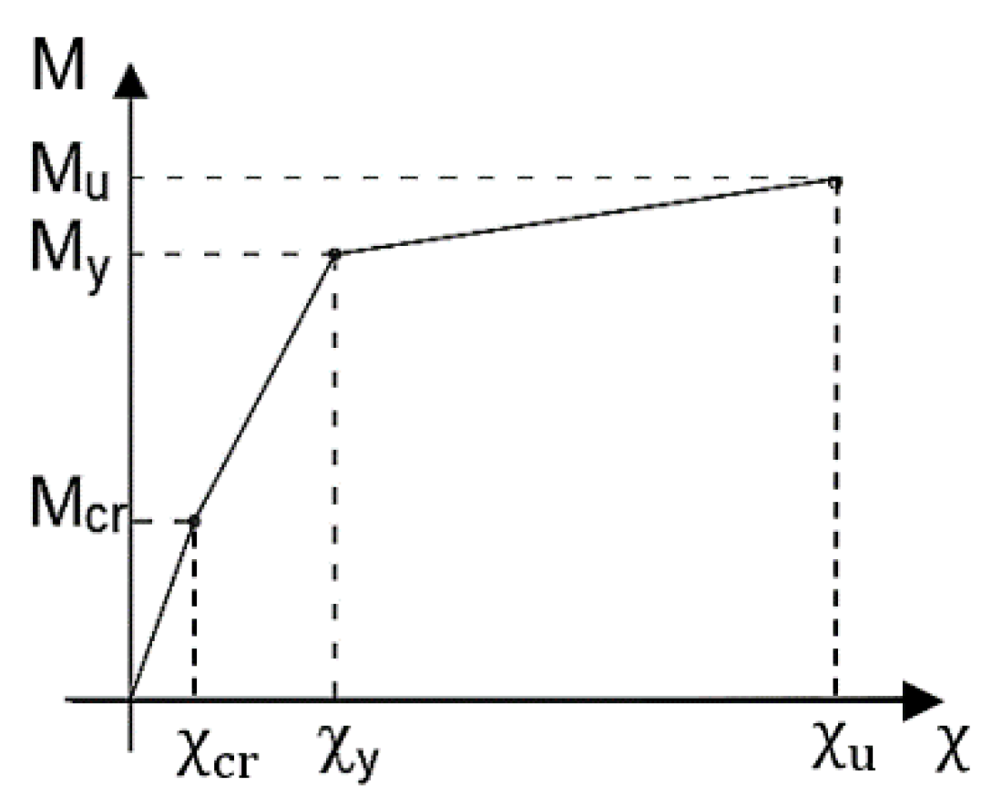
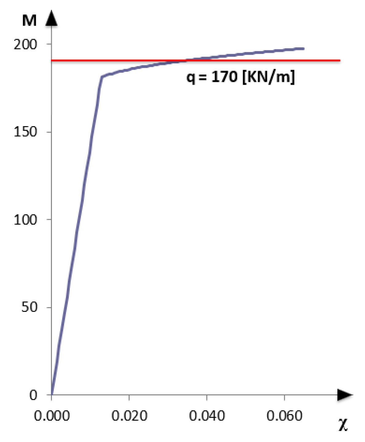
- First uncracked elastic phase, with a pattern close to the linear and curvature ranging from 0 to χcr. The tensed concrete contributes to the resistance of the structure up to the cracking bending moment (Mcr), where stress in concrete in tension exceeds its tensile strength;
- Second phase with cracked section, bending moment ranging from the cracking bending moment (Mcr) and the reinforcement yielding bending moment (My), increasing levels of curvature and higher deformability;
- Third phase with yielded reinforcements, showing a rapid increase of the curvature pattern until the ultimate bending moment (Mu) is reached when one of the two materials, reinforcing steel or concrete, experiences the maximum nominal strain.
3. Basics of iFEM
4. iFEM Algorithm with Material Nonlinearity
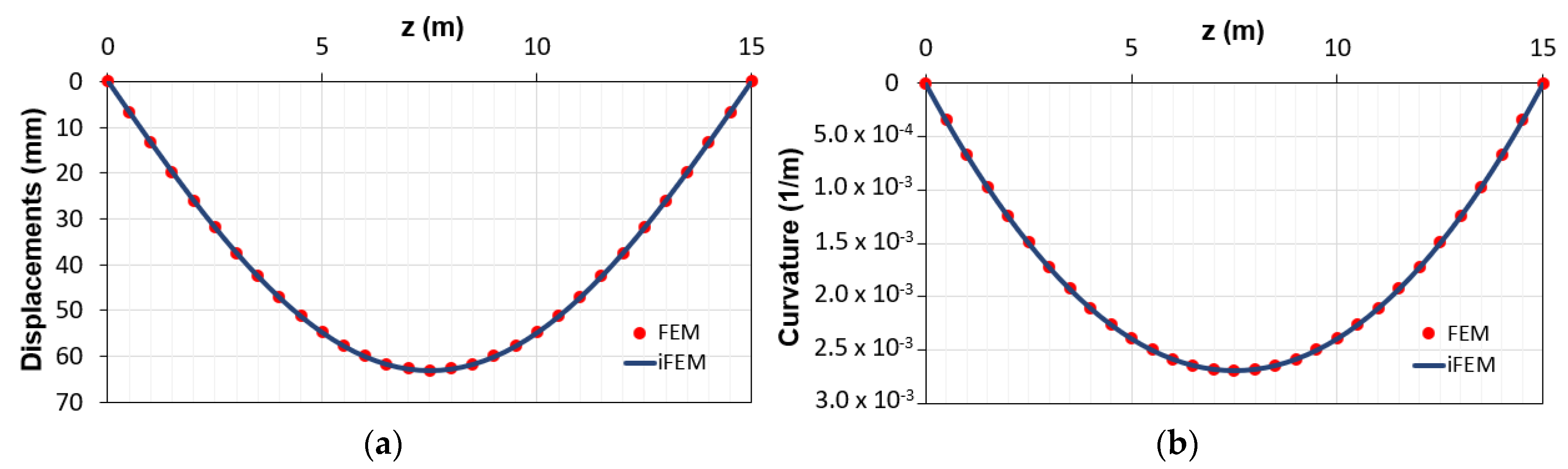
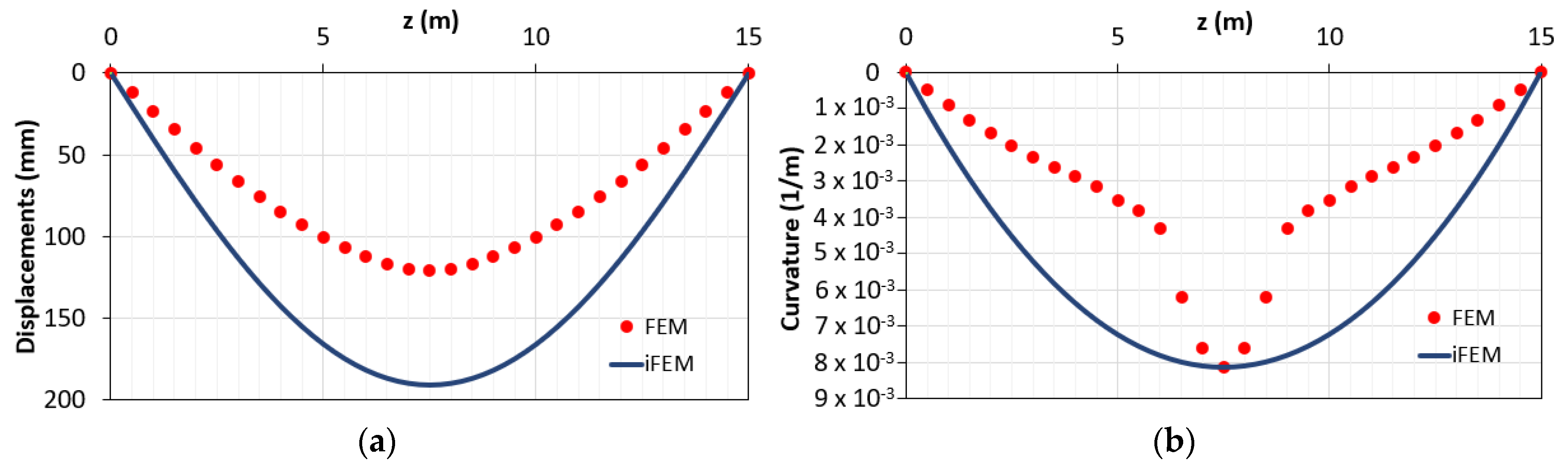
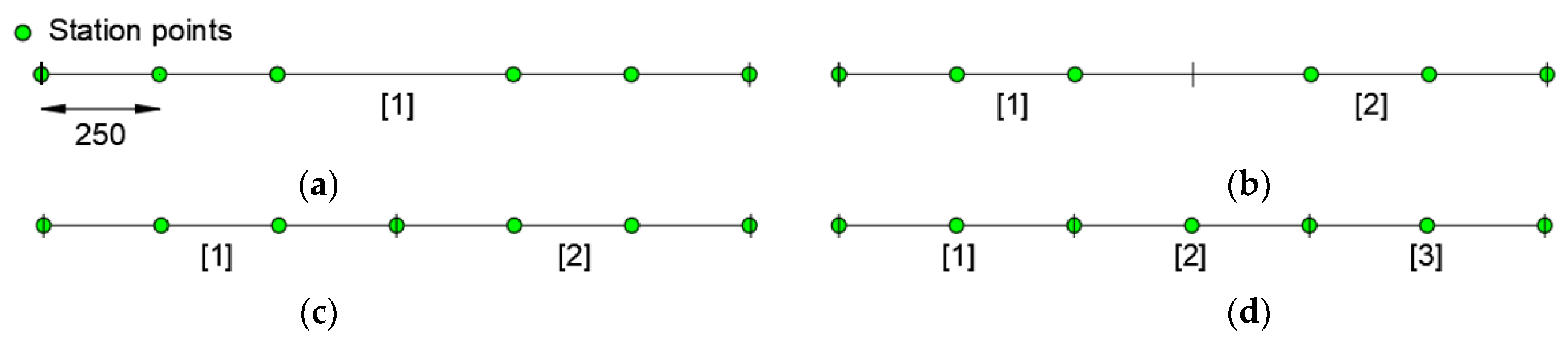
4.1. Statically Determinate Structures
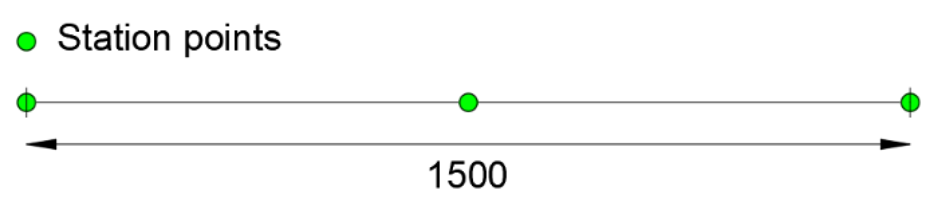
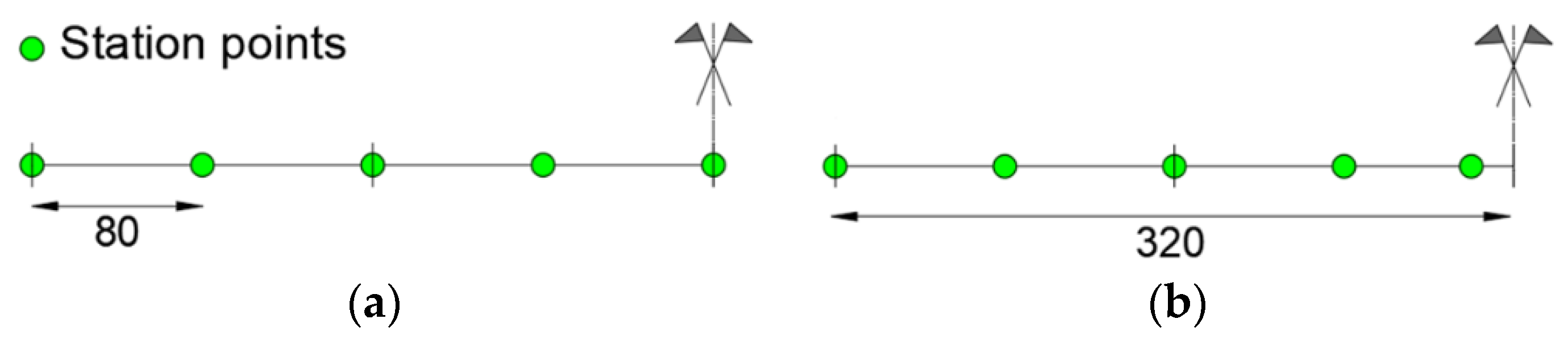
- not all the station points belong to zones with the same behavior (1st–2nd or yielding phase);
- each span with a different behavior needs to be modeled with a different inverse element.
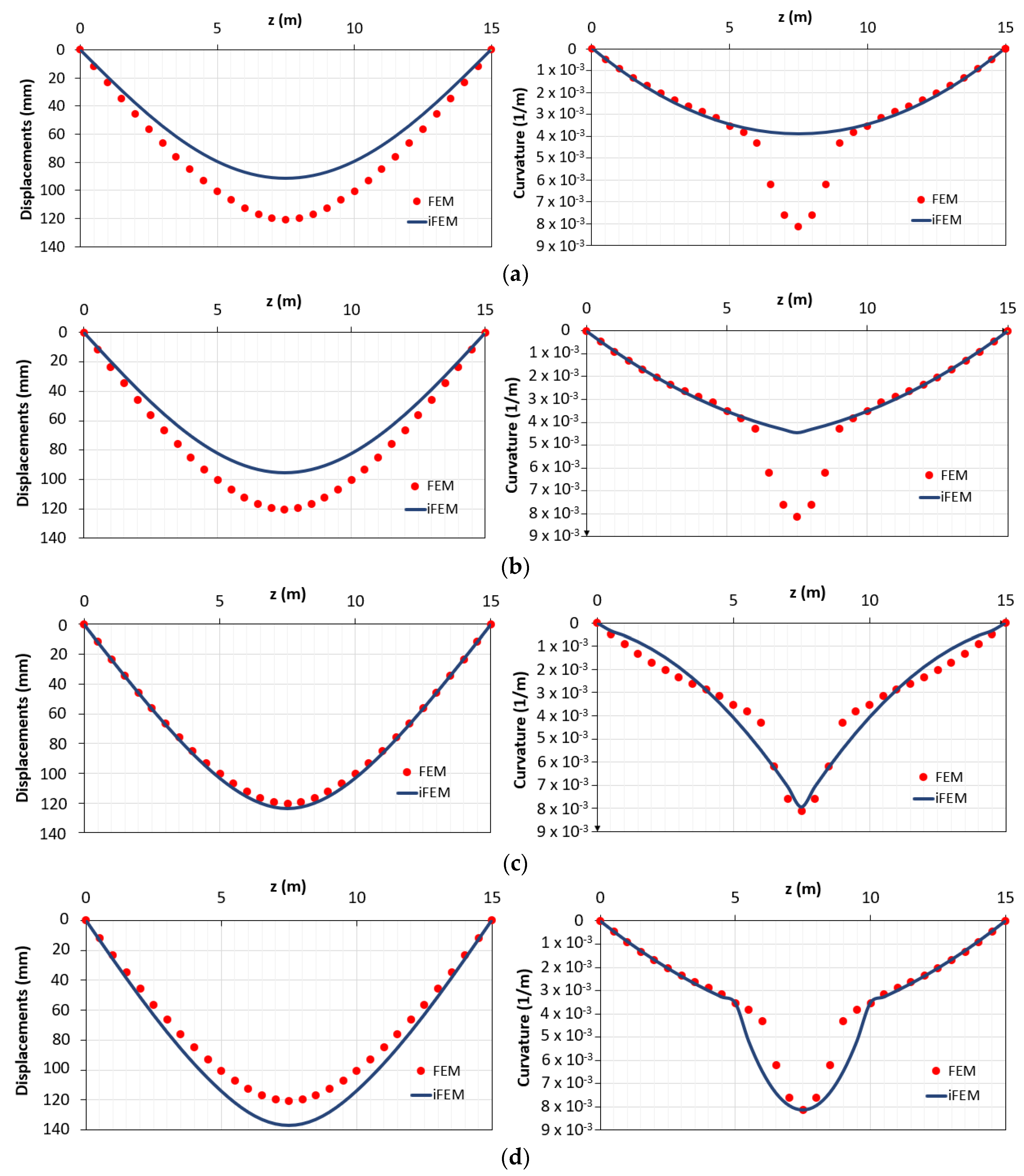
4.1.1. Hybrid Method for Statically Determinate Structures
- Find the initial curvature measurement (from the strain measurements) and using the bending moment-curvature diagram, get the corresponding bending moment value at the station points;
- Reconstruct the bending moment diagram along the whole beam span with a polynomial function interpolating the values obtained in step (1). In the case of l estimated bending moment values, the polynomial function M(z) has the form:
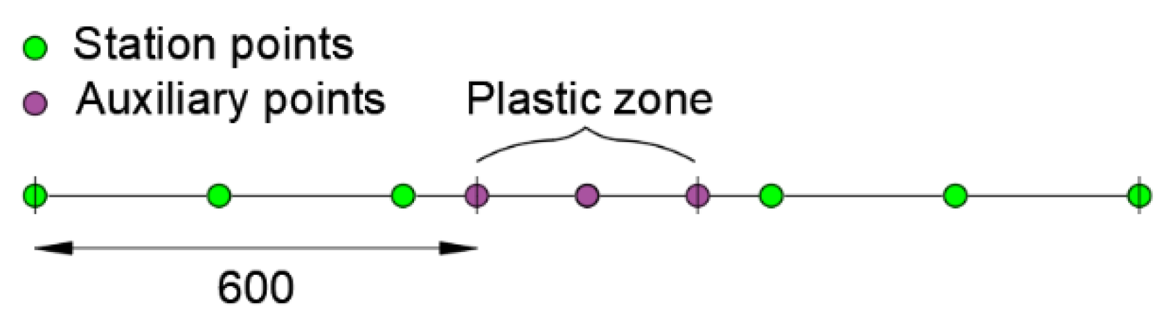
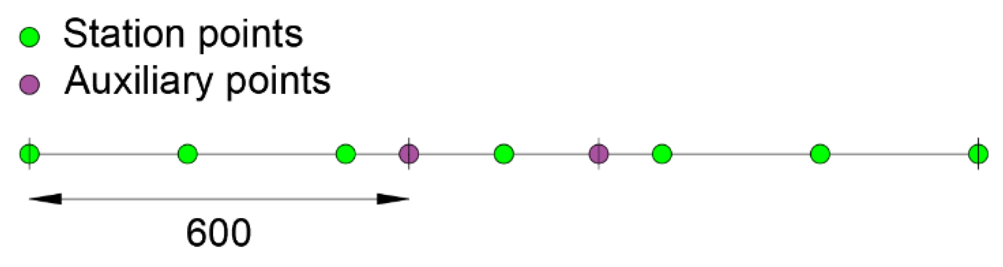
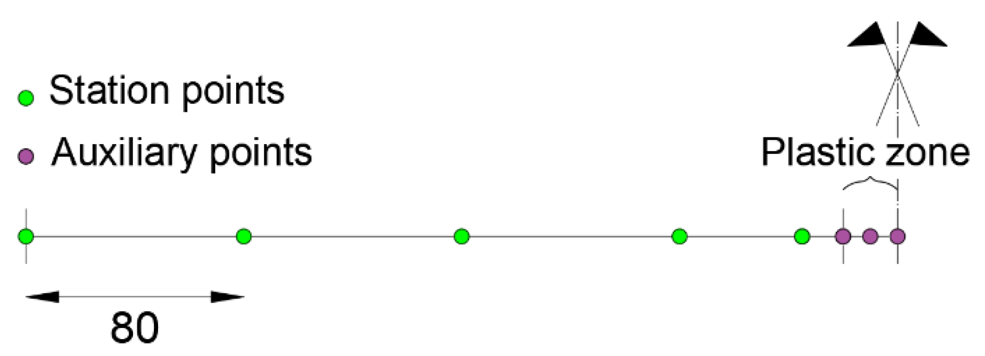
- Identify the beginning and the end of the plastic zone by comparing the values of the bending moment diagram and My (the plastic zone must correspond to an inverse element characterized by “auxiliary points”, i.e., additional station points);
- Evaluate the curvatures and the bending moment values at the auxiliary points considering the bending moment-curvature diagram;
- Perform iFEM analysis using the measured and estimated (auxiliary points) curvatures as input data.
4.2. Statically Indeterminate Structures
- Check of the curvatures to model each zone in a different phase with its inverse element;
- A procedure that allows obtaining the curvatures in the plastic zone if this exhibits a lack of station points.
Hybrid Method for Statically Indeterminate Structures
- Perform the iFEM analysis with the input data from the strain sensors (FEM simulated) outside the plasticized areas (checking curvatures lower than yielding curvatures) and identify the exact length of the plastic areas;
- Estimate the input data in the plasticized areas (auxiliary station points) from a direct local FEM analysis of a reduced statically determinate scheme, having at the edge of the model (beginning/end of the plastic areas) an imposed load conditions given by transverse displacement and rotation predicted by the iFEM analysis;
- Perform a new iFEM analysis with the initial input data and the estimated value for the plasticized area (auxiliary station points from data simulated by the local FE model).
5. Conclusions
Author Contributions
Funding
Institutional Review Board Statement
Informed Consent Statement
Data Availability Statement
Conflicts of Interest
References
- Lynch, J.P.; Loh, K.J. A summary review of wireless sensors and sensor networks for structural health monitoring. Shock Vib. Dig. 2006, 38, 91–128. [Google Scholar] [CrossRef]
- Tondolo, F.; Cesetti, A.; Matta, E.; Quattrone, A.; Sabia, D. Smart reinforcement steel bars with low-cost MEMS sensors for the structural health monitoring of RC structures. Constr. Build. Mater. 2018, 173, 740–753. [Google Scholar] [CrossRef]
- Tondolo, F.; Matta, E.; Quattrone, A.; Sabia, D. Experimental test on an RC beam equipped with embedded barometric pressure sensors for strains measurement. Smart Mater. Struct. 2019, 28, 055040. [Google Scholar] [CrossRef]
- Ko, W.L.; Richards, W.L.; Fleischer, V.T. Applications of the Ko Displacement Theory to the Deformed Shape Predictions of the Doubly-Tapered Ikhana Wing. 2009; p. 214652. Available online: https://ntrs.nasa.gov/citations/20090040594 (accessed on 12 January 2021).
- Kang, L.H.; Kim, D.K.; Han, J.H. Estimation of dynamic structural displacements using fiber Bragg grating strain sensors. J. Sound Vib. 2007, 305, 534–542. [Google Scholar] [CrossRef]
- Bruno, R.; Toomarian, N.; Salama, M. Shape estimation from incomplete measurements: A neural-net approach. Smart Mater. Struct. 1994, 3, 92–97. [Google Scholar] [CrossRef]
- Tessler, A.; Spangler, J.L. A Variational Principal for Reconstruction of Elastic Deformation of Shear Deformable Plates and Shells; NASA Technical Memorandum, Langley Research Center: Hampton, VA, USA, 2003; p. 212445.
- Tessler, A.; Spangler, J.L. A least-squares variational method for full-field reconstruction of elastic deformations in shear-deformable plates and shells. Comput. Methods Appl. Mech. Eng. 2005, 194, 327–339. [Google Scholar] [CrossRef]
- Kefal, A.; Oterkus, E.; Tessler, A.; Spangler, J.L. A quadrilateral inverse-shell element with drilling degrees of freedom for shape sensing and structural health monitoring. Eng. Sci. Technol. Int. J. 2016, 19, 1299–1313. [Google Scholar] [CrossRef]
- Kefal, A. An efficient curved inverse-shell element for shape sensing and structural health monitoring of cylindrical marine structures. Ocean Eng. 2019, 188, 106262. [Google Scholar] [CrossRef]
- Kefal, A.; Oterkus, E. Isogeometric iFEM Analysis of Thin Shell Structures. Sensors 2020, 20, 2685. [Google Scholar] [CrossRef] [PubMed]
- Zhao, F.; Xu, L.; Bao, H.; Du, J. Shape sensing of variable cross-section beam using the inverse finite element method and isogeometric analysis. Measurement 2020, 158, 107656. [Google Scholar] [CrossRef]
- Gherlone, M. Beam Inverse Finite Element Formulation. LAQ Report 2008; Politecnico di Torino: Torino, Italy, 2008. [Google Scholar]
- Gherlone, M.; Cerracchio, P.; Mattone, M.; Di Sciuva, M.; Tessler, A. Shape sensing of 3D frame structures using an inverse finite element method. Int. J. Solid Struct. 2012, 49, 3100–3112. [Google Scholar] [CrossRef]
- Savino, P.; Gherlone, M.; Tondolo, F. Shape sensing with inverse Finite Element Method for slender structures. Struct. Eng. Mech. 2019, 72, 217–227. [Google Scholar]
- Savino, P.; Tondolo, F.; Gherlone, M.; Tessler, A. Application of Inverse Finite Element Method to Shape Sensing of Curved Beams. Sensors 2020, 20, 7012. [Google Scholar] [CrossRef] [PubMed]
- Tessler, A.; Roy, R.; Esposito, M.; Surace, C.; Gherlone, M. Shape sensing of plate and shell structures undergoing large displacements using the inverse Finite Element Method. Shock Vib. 2018, 2018, 8076085. [Google Scholar] [CrossRef]
- Quach, C.C.; Vazquez, S.L.; Tessler, A.; Moore, J.P.; Cooper, E.G.; Spangler, J.L. Structural anomaly detection using fiber optic sensors and inverse finite element method. In Proceedings of the AIAA Guidance, Navigation, and Control Conference and Exhibit, San Francisco, CA, USA, 15–18 August 2005. [Google Scholar]
- Vazquez, S.L.; Tessler, A.; Quach, C.C.; Cooper, E.G.; Parks, J.; Spangler, J.L. Structural Health Monitoring Using High-Density Fiber Optic Strain Sensor and Inverse Finite Element Methods; NASA Technical Memorandum, Langley Research Center: Hampton, VA, USA, 2005.
- Cerracchio, P.; Gherlone, M.; Tessler, A. Real-time displacement monitoring of a composite stiffened panel subjected to mechanical and thermal loads. Meccanica 2015, 50, 2487–2496. [Google Scholar] [CrossRef]
- Kefal, A.; Oterkus, E. Structural health monitoring of marine structures by using inverse finite element method. In Proceedings of the 5th International Conference on Marine Structures (MARSTRUCT), Southampton, UK, 25–27 March 2015. [Google Scholar]
- Kefal, A.; Oterkus, E. Displacement and stress monitoring of a chemical tanker based on inverse finite element method. Ocean Eng. 2016, 112, 33–46. [Google Scholar] [CrossRef]
- Kefal, A.; Oterkus, E. Displacement and stress monitoring of a Panamax containership using inverse finite element method. Ocean Eng. 2016, 119, 16–29. [Google Scholar] [CrossRef]
- Li, M.; Kefal, A.; Oterkus, E.; Oterkus, S. Structural health monitoring of an offshore wind turbine tower using iFEM methodology. Ocean Eng. 2020, 204, 107291. [Google Scholar] [CrossRef]
- Gherlone, M.; Cerracchio, P.; Mattone, M. Shape sensing methods: Review and experimental comparison on a wing-shaped plate. Prog. Aerosp. Sci. 2018, 99, 14–26. [Google Scholar] [CrossRef]
- Gherlone, M.; Cerracchio, P.; Mattone, M.; Di Sciuva, M.; Tessler, A. An inverse finite element method for beam shape sensing: Theoretical framework and experimental validation. Smart Mater. Struct. 2014, 23, 045027. [Google Scholar] [CrossRef]
- Zhao, Y.; Bao, H.; Duan, X.; Fang, H. The application research of inverse Finite Element Method for frame deformation estimation. Int. J. Aerosp. Eng. 2017, 2017, 1326309. [Google Scholar] [CrossRef]
- Esposito, M.; Gherlone, M. Composite wing box deformed-shape reconstruction based on measured strains: Optimization and comparison of existing approaches. Aerosp. Sci. Technol. 2020, 99, 105758. [Google Scholar] [CrossRef]


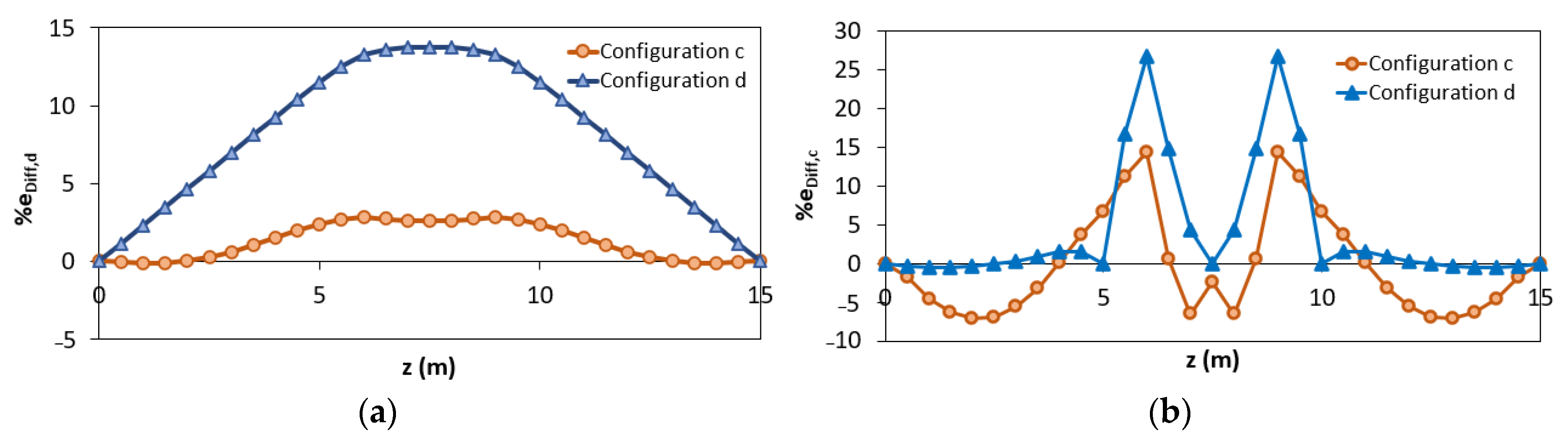
| Configurations | eRMS,d (%) | eRMS,c (%) |
|---|---|---|
| a | 14.76 | 16.82 |
| b | 12.67 | 14.59 |
| c | 1.72 | 6.32 |
| d | 9.21 | 8.77 |
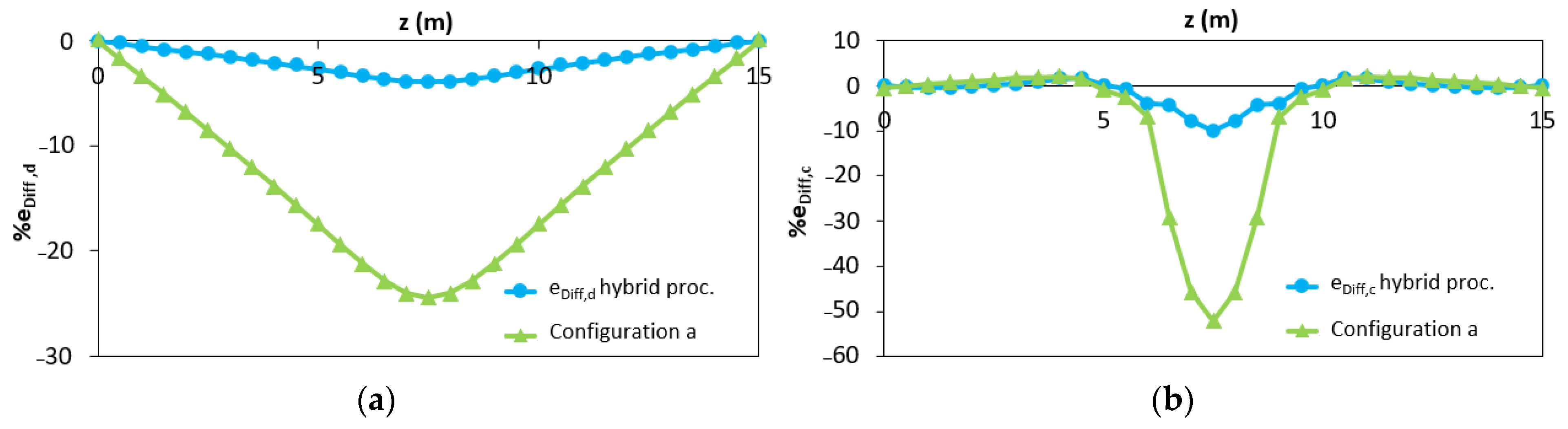
| Configurations | eRMS,d (%) | eRMS,c (%) |
|---|---|---|
| a | 33.03 | 13.45 |
| b | 1.62 | 8.80 |
Publisher’s Note: MDPI stays neutral with regard to jurisdictional claims in published maps and institutional affiliations. |
© 2021 by the authors. Licensee MDPI, Basel, Switzerland. This article is an open access article distributed under the terms and conditions of the Creative Commons Attribution (CC BY) license (http://creativecommons.org/licenses/by/4.0/).
Share and Cite
Savino, P.; Gherlone, M.; Tondolo, F.; Greco, R. Shape-Sensing of Beam Elements Undergoing Material Nonlinearities. Sensors 2021, 21, 528. https://doi.org/10.3390/s21020528
Savino P, Gherlone M, Tondolo F, Greco R. Shape-Sensing of Beam Elements Undergoing Material Nonlinearities. Sensors. 2021; 21(2):528. https://doi.org/10.3390/s21020528
Chicago/Turabian StyleSavino, Pierclaudio, Marco Gherlone, Francesco Tondolo, and Rita Greco. 2021. "Shape-Sensing of Beam Elements Undergoing Material Nonlinearities" Sensors 21, no. 2: 528. https://doi.org/10.3390/s21020528
APA StyleSavino, P., Gherlone, M., Tondolo, F., & Greco, R. (2021). Shape-Sensing of Beam Elements Undergoing Material Nonlinearities. Sensors, 21(2), 528. https://doi.org/10.3390/s21020528