
Health Monitoring of Aerospace Structures Utilizing Novel Health Indicators Extracted from Complex Strain and Acoustic Emission Data

 ,
, 

Abstract
:1. Introduction
1.1. State of the Art
1.1.1. Fiber Optical Sensors
1.1.2. Acoustic Emission
1.1.3. Health Indicators
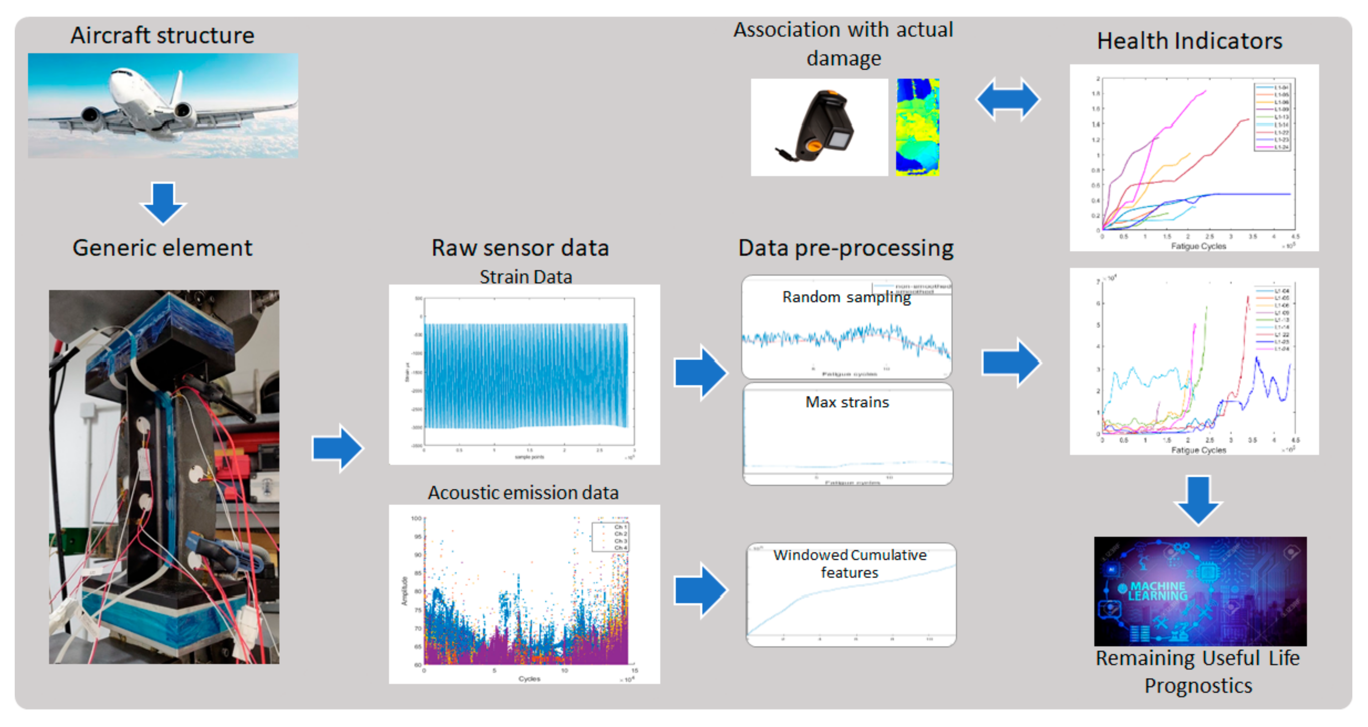
2. Experimental Procedure
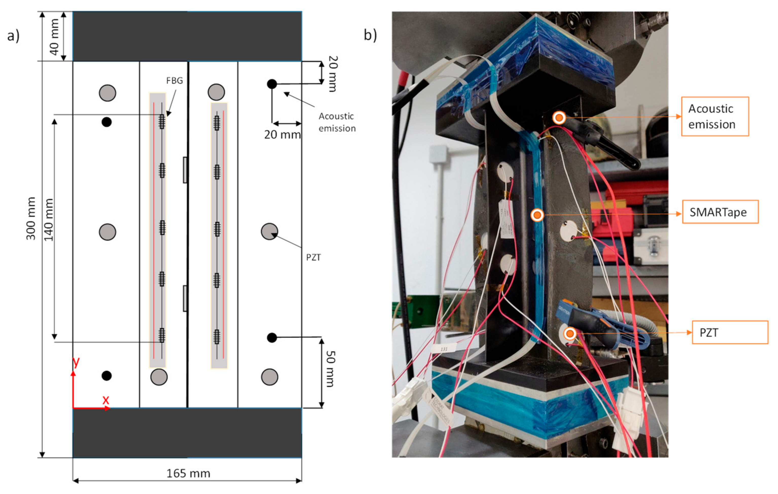
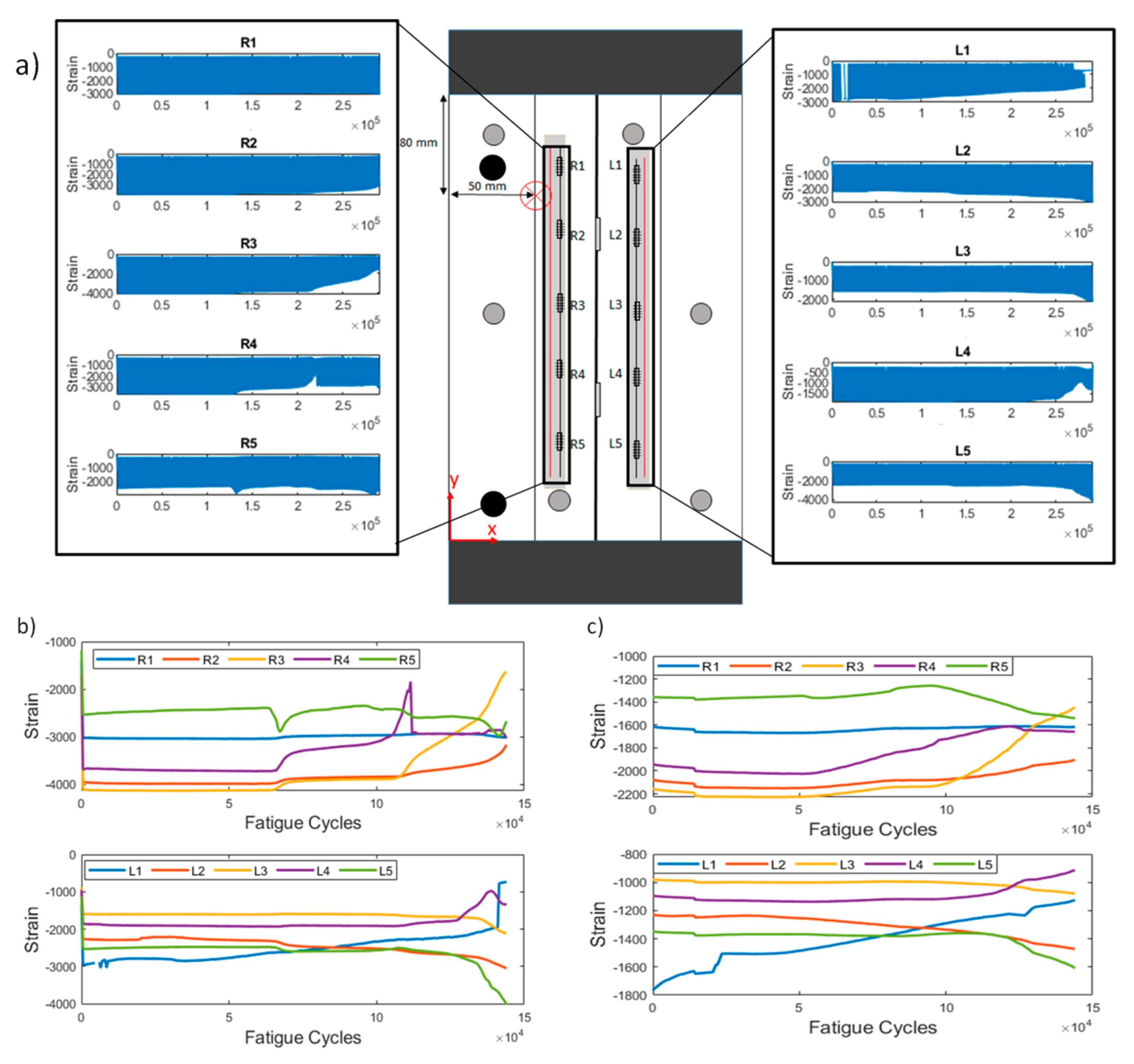
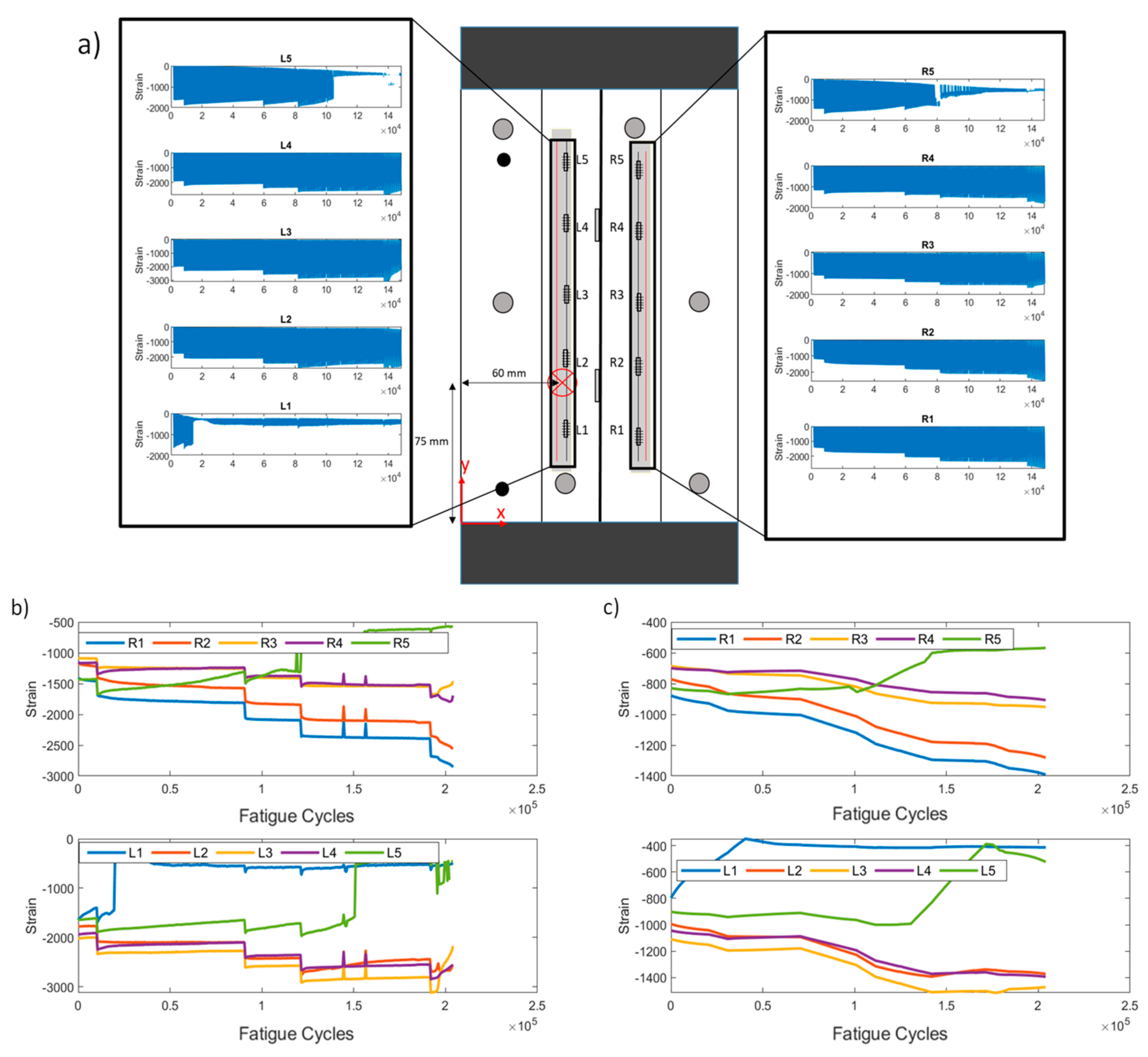
2.1. Test Article Definition
2.2. Test Campaign
2.3. SHM Data Pre-Processing
3. Methodologies—Health Indicator Development
3.1. Strain Based HIs
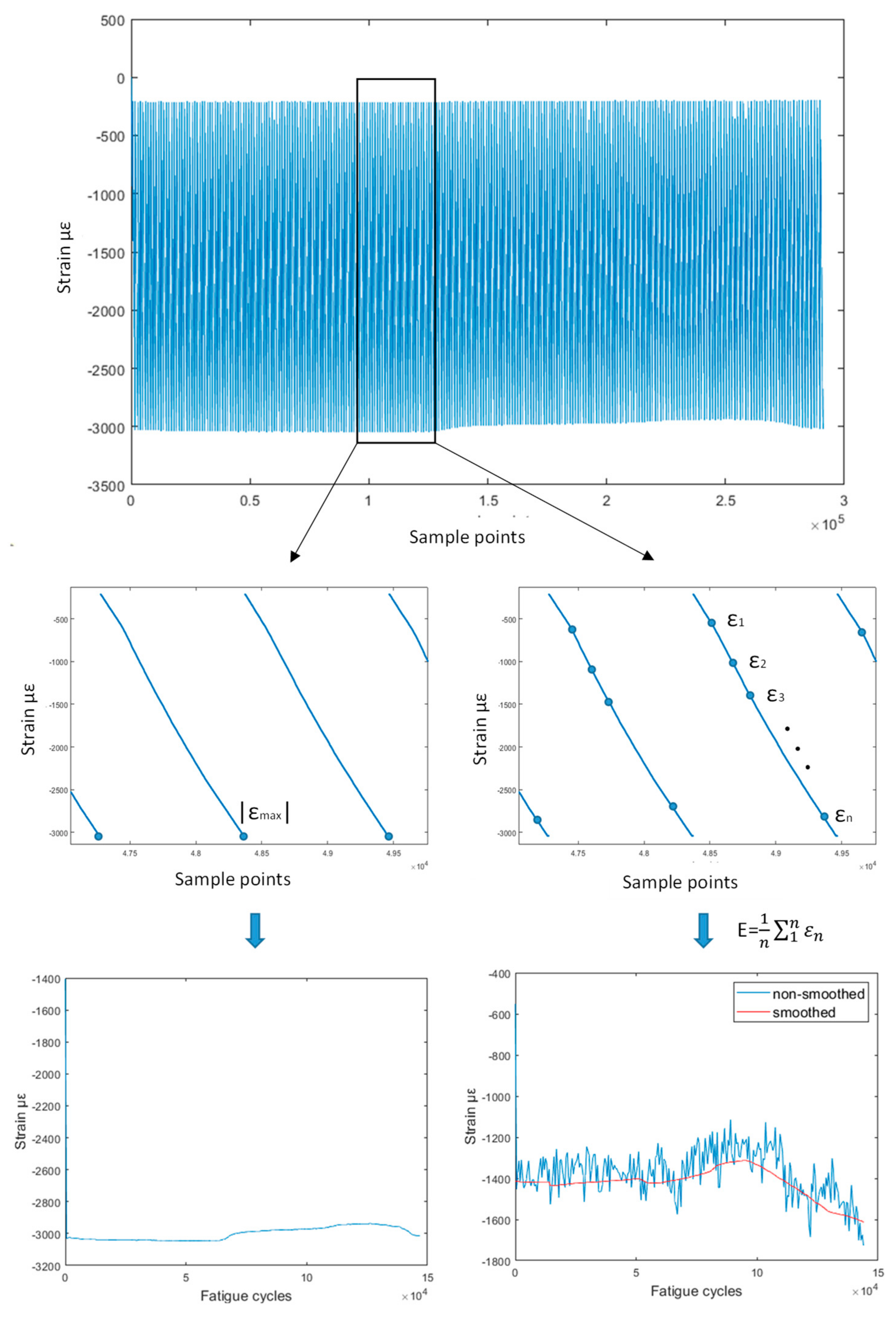
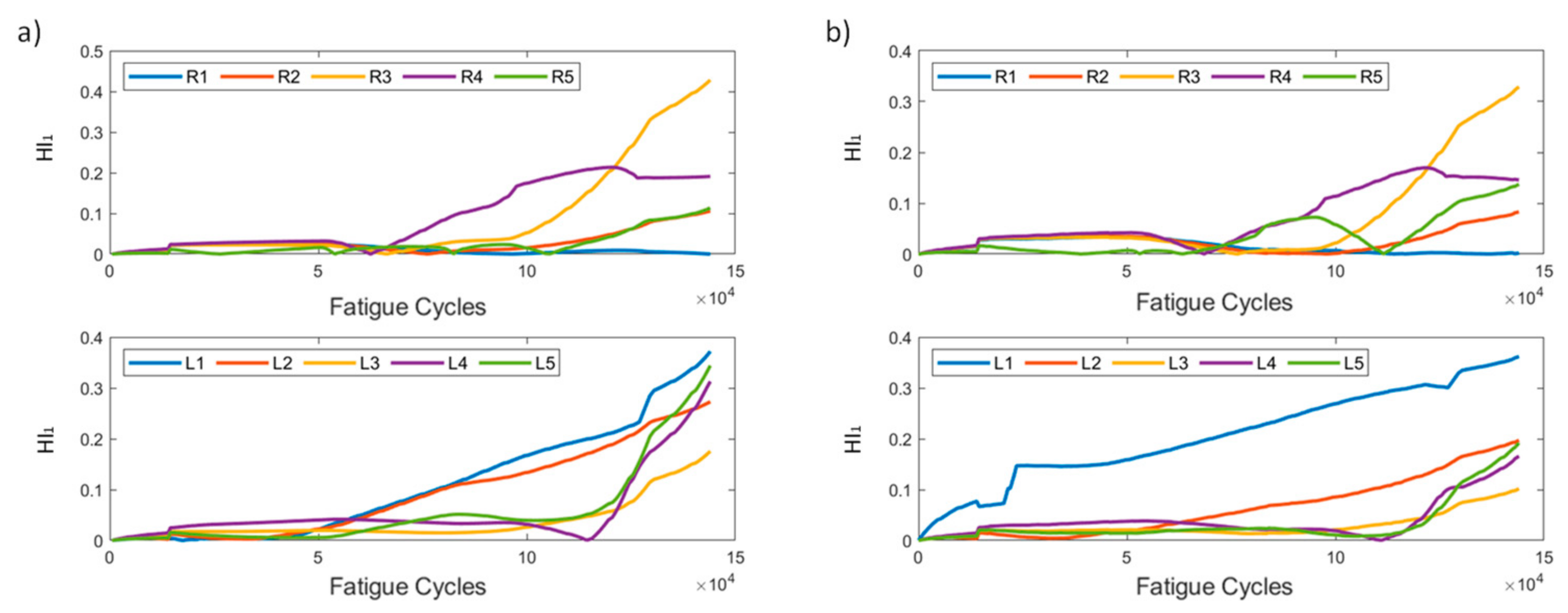
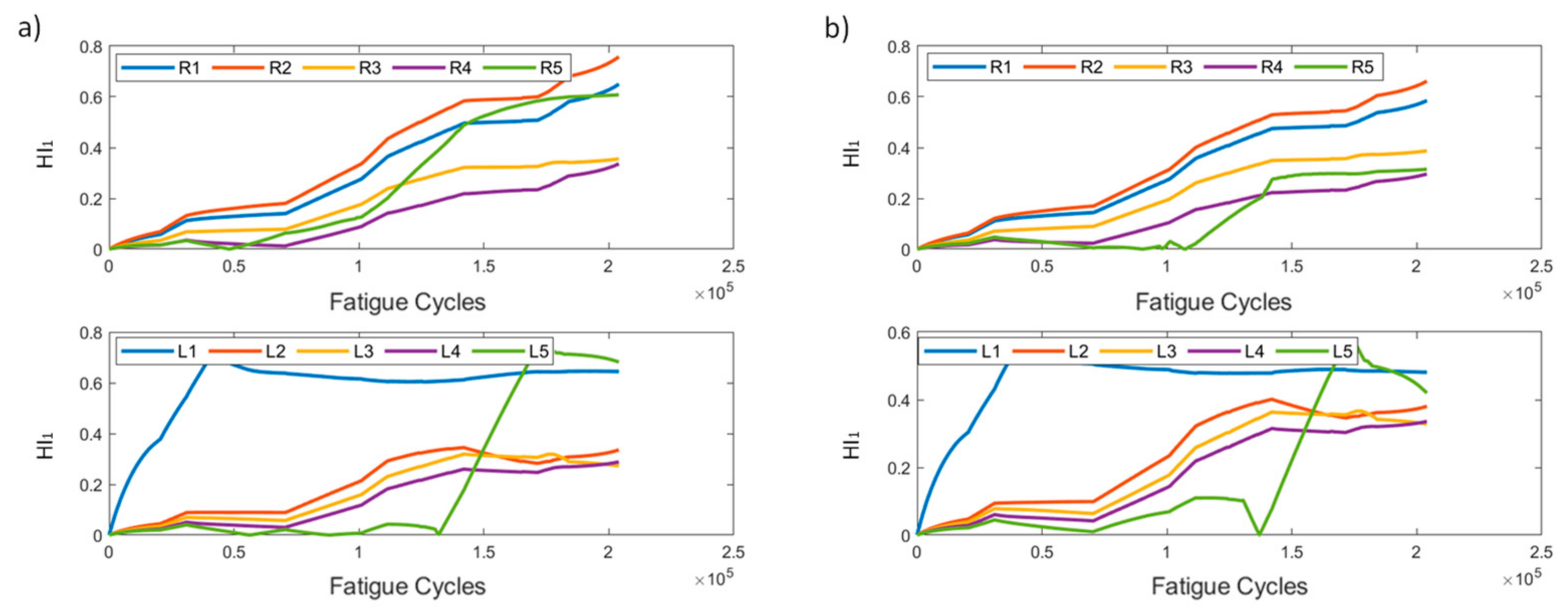
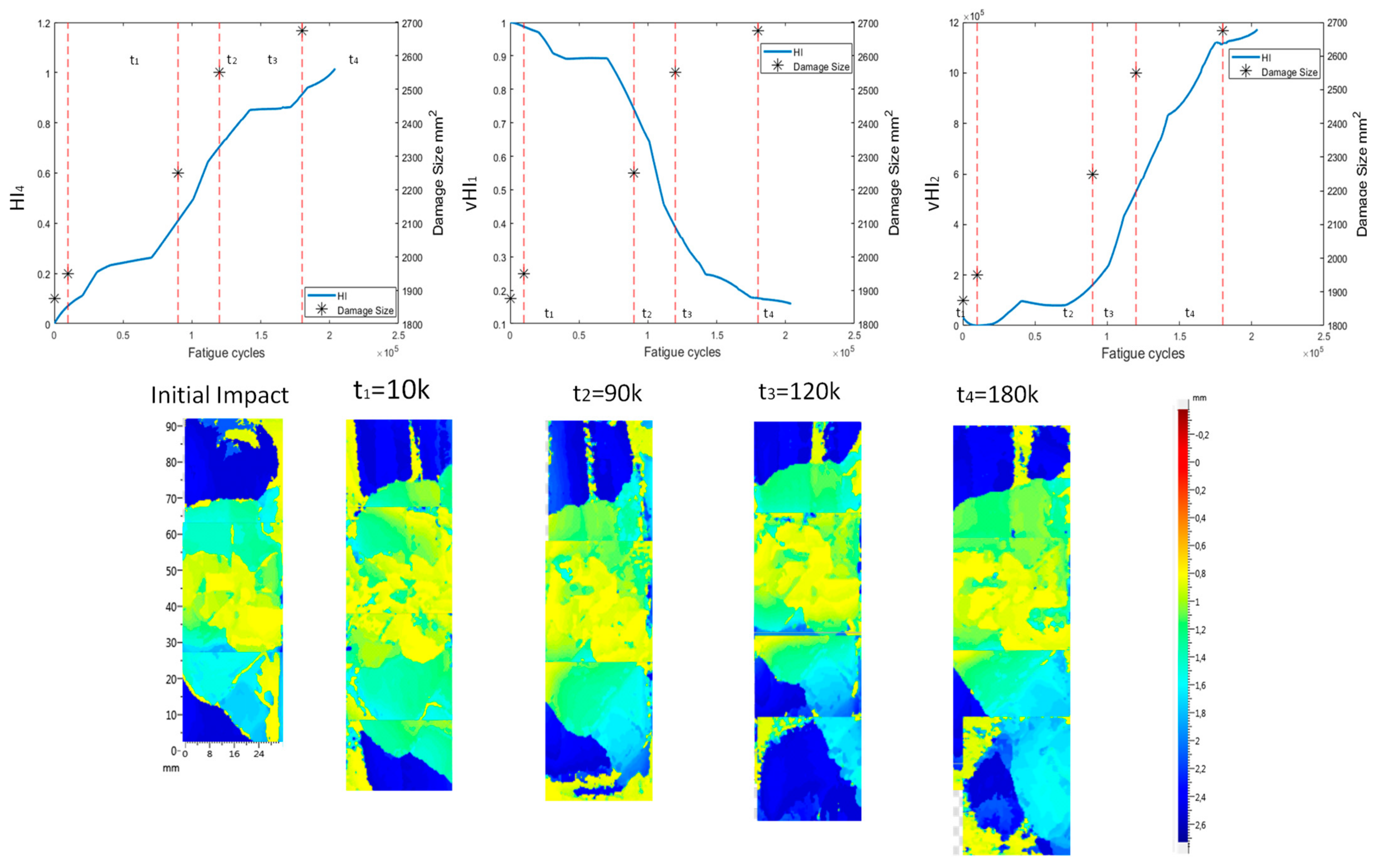
3.1.1. HI1
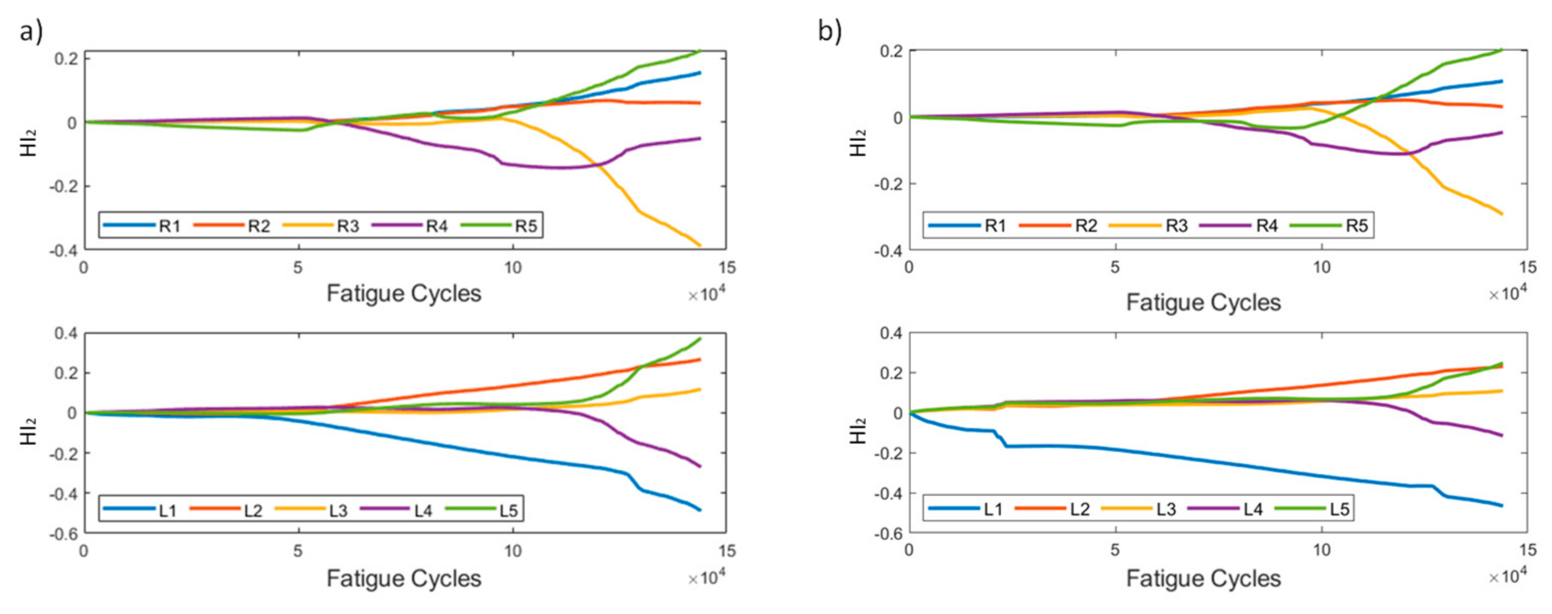
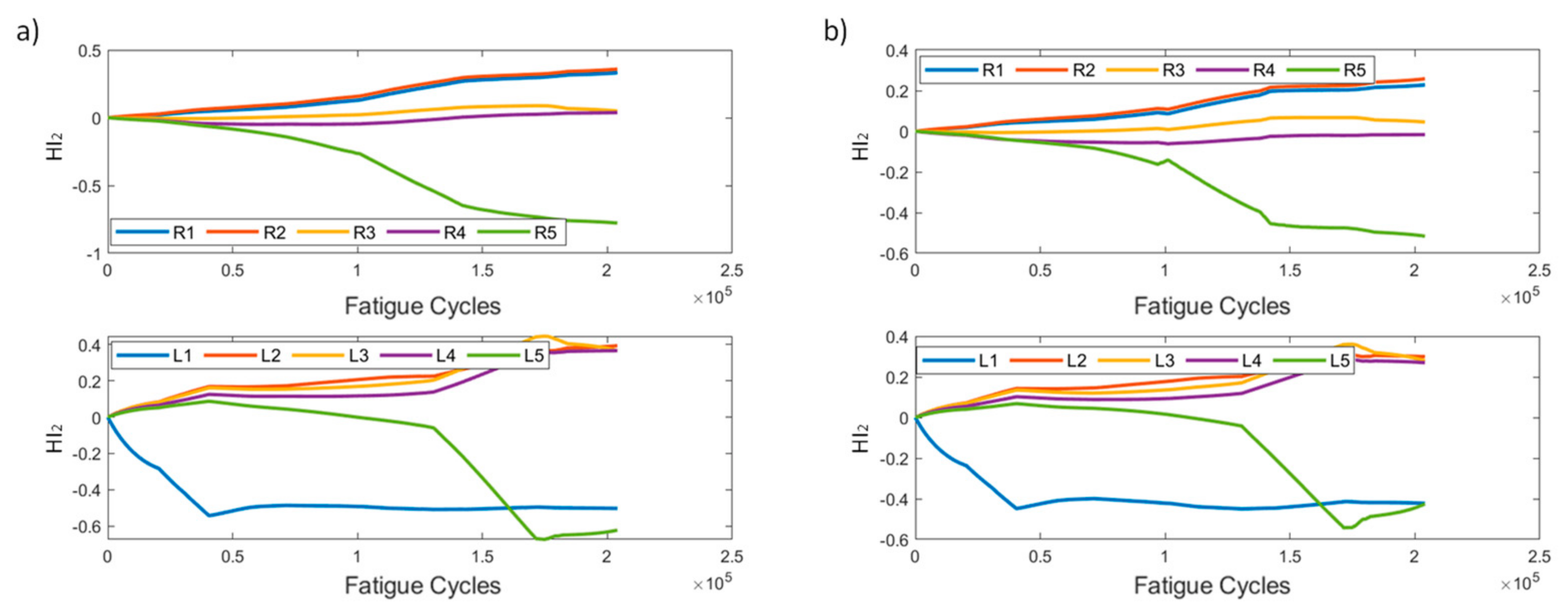
3.1.2. HI2
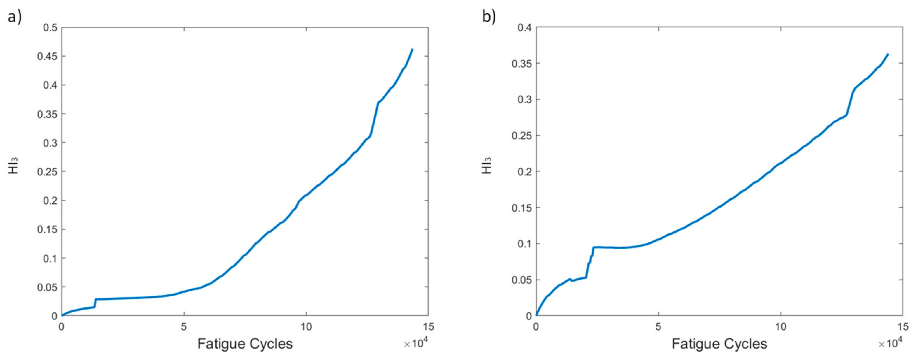
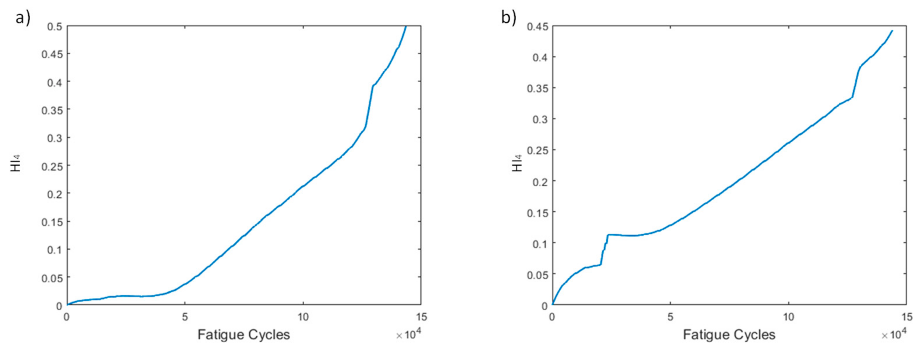
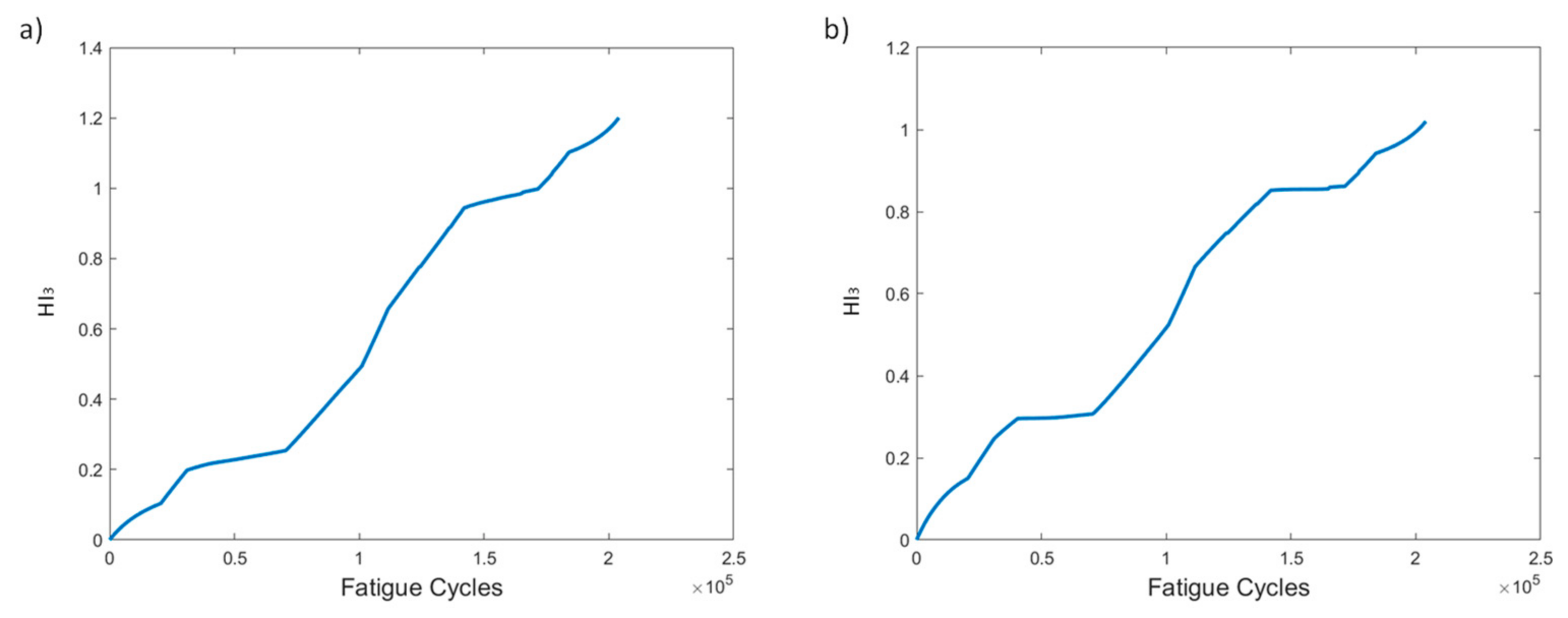
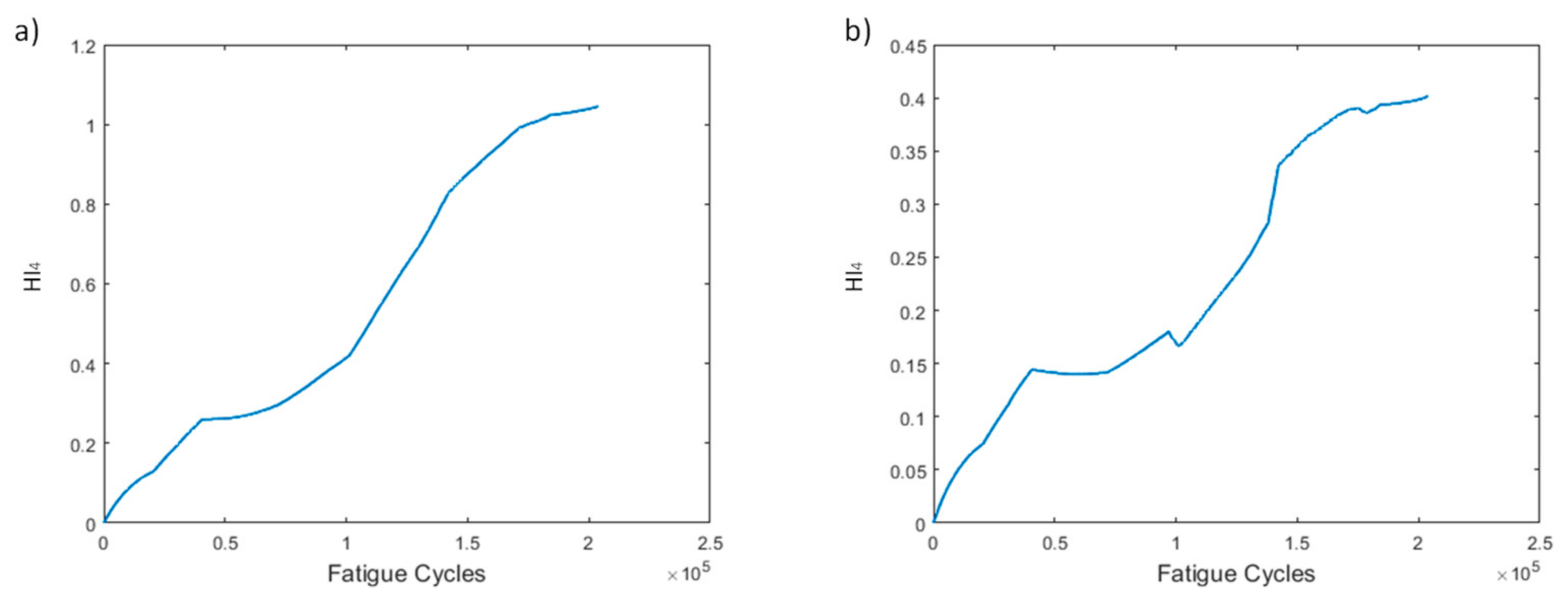
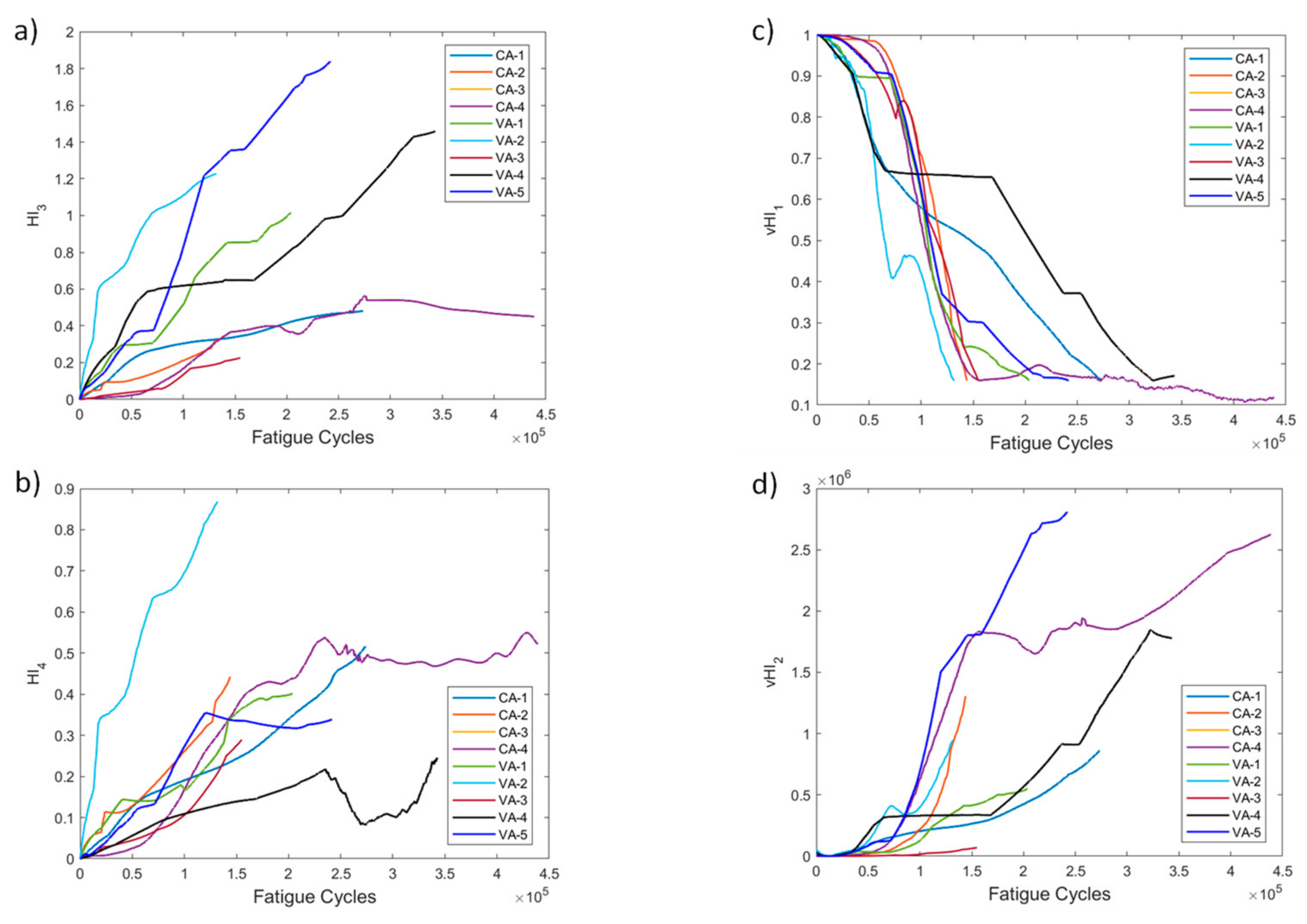
3.1.3. HI3 and HI4
3.2. Virtual Health Indicators
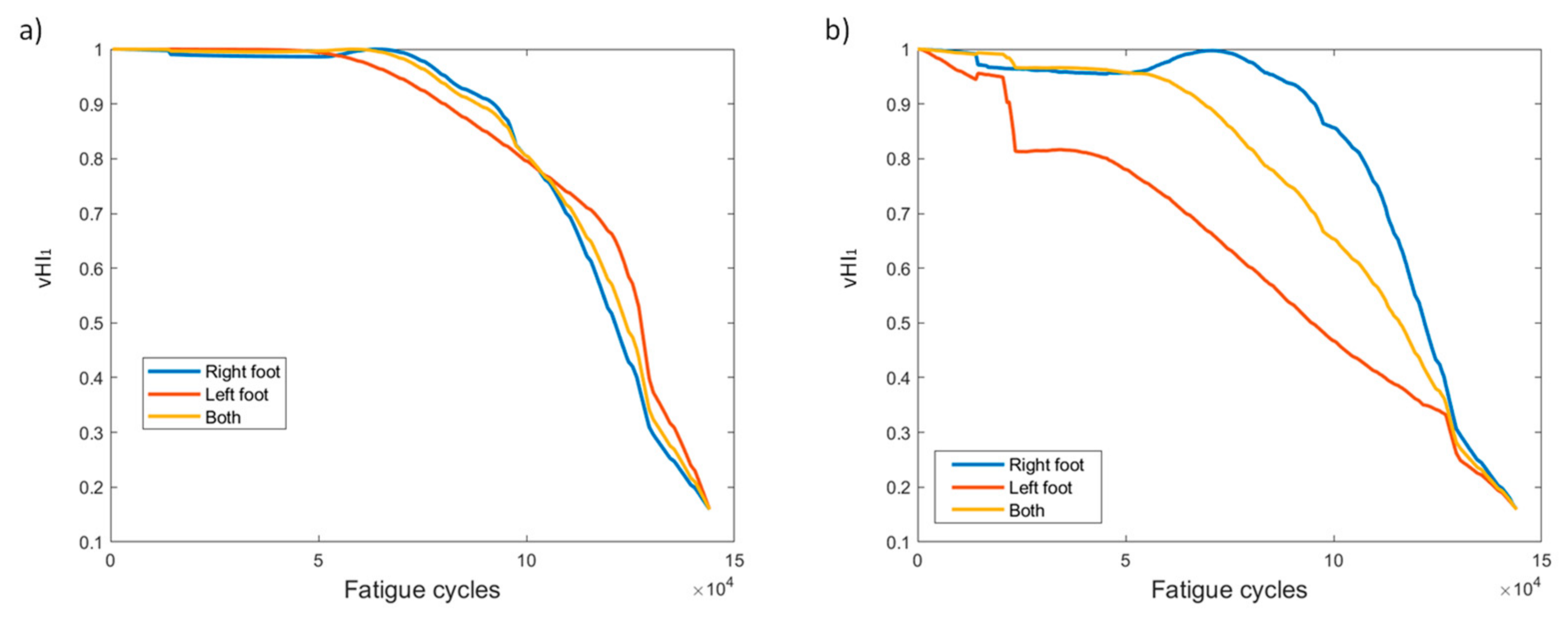
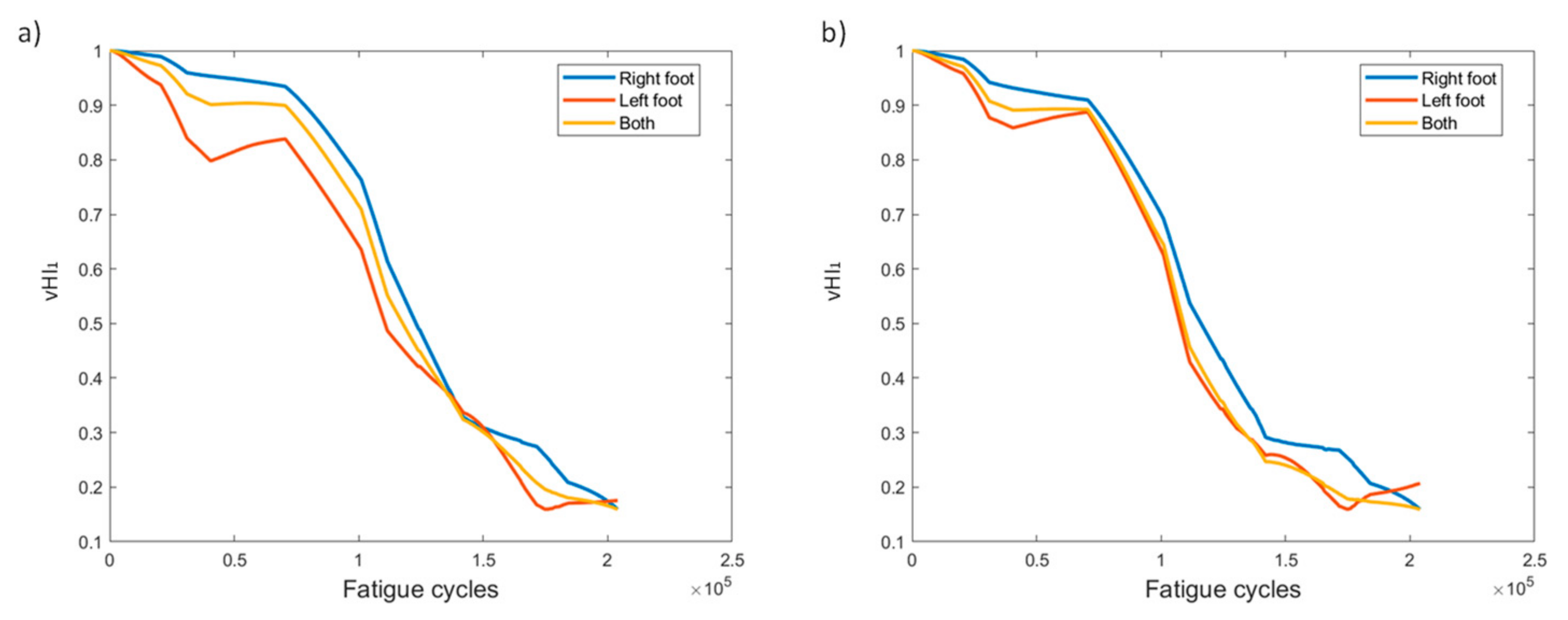
3.2.1. vHI1
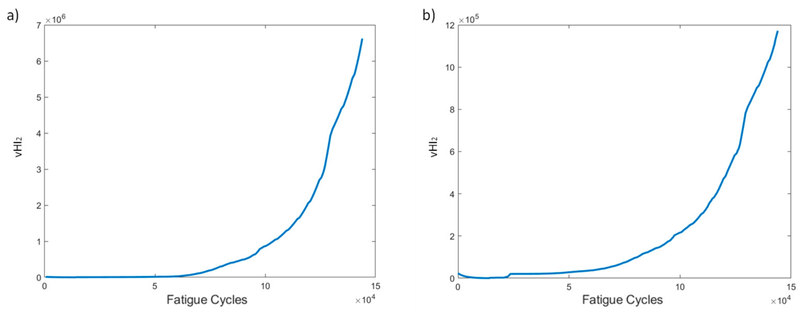
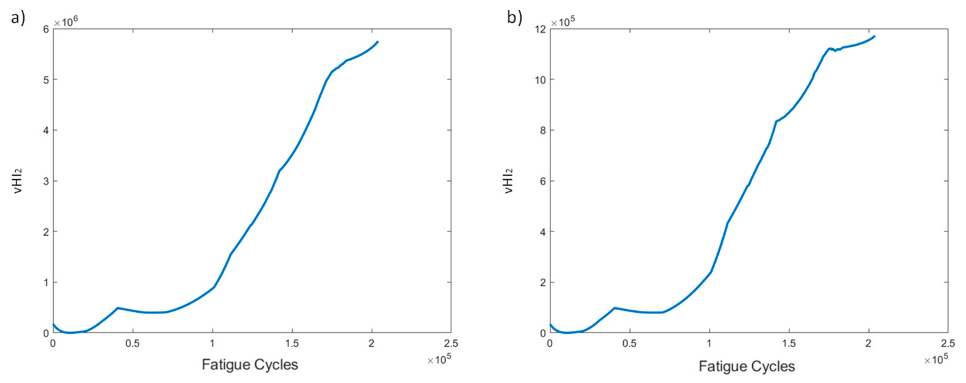
3.2.2. vHI2
- The initial portion of the sensor data matrix X considered as reference Xref is normalized to zero mean and unit variance. The mean Mref and the variance Vref are saved for later use.
- A PCA model is created using Xref and the coefficients matrix Pmxn is calculated, where m represents the time points and n the number of sensors. The reduced matrix Prmxk is saved where k is the number of components whose explained variance is over 90%.
- Then Mref and Vref are used to scale the full dataset X, and Pr is used to transform the normalized data to the PC space as in T = .
- Then, the reconstructed matrix Xr is calculated where Xr = T + R and R is the reconstruction error.
- Q is calculated in Equation (9):where i = 1, …, N is the ith FBG sensor, and and the original and reconstructed data, respectively, at time t.
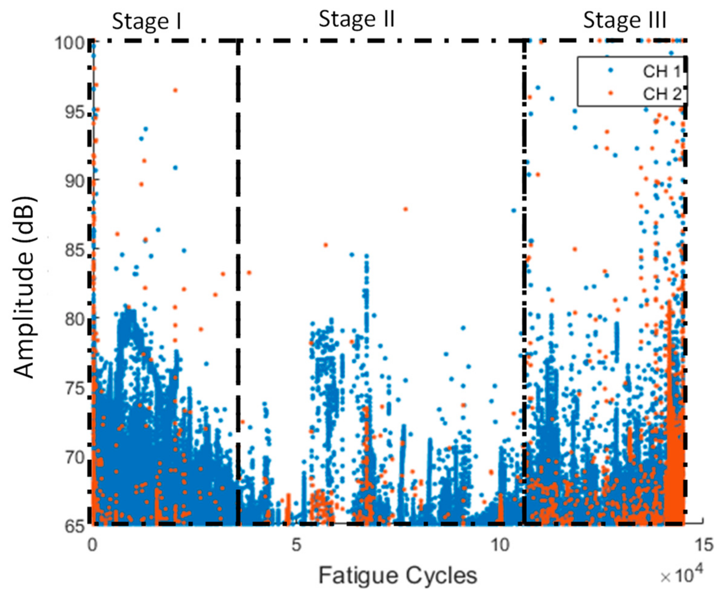
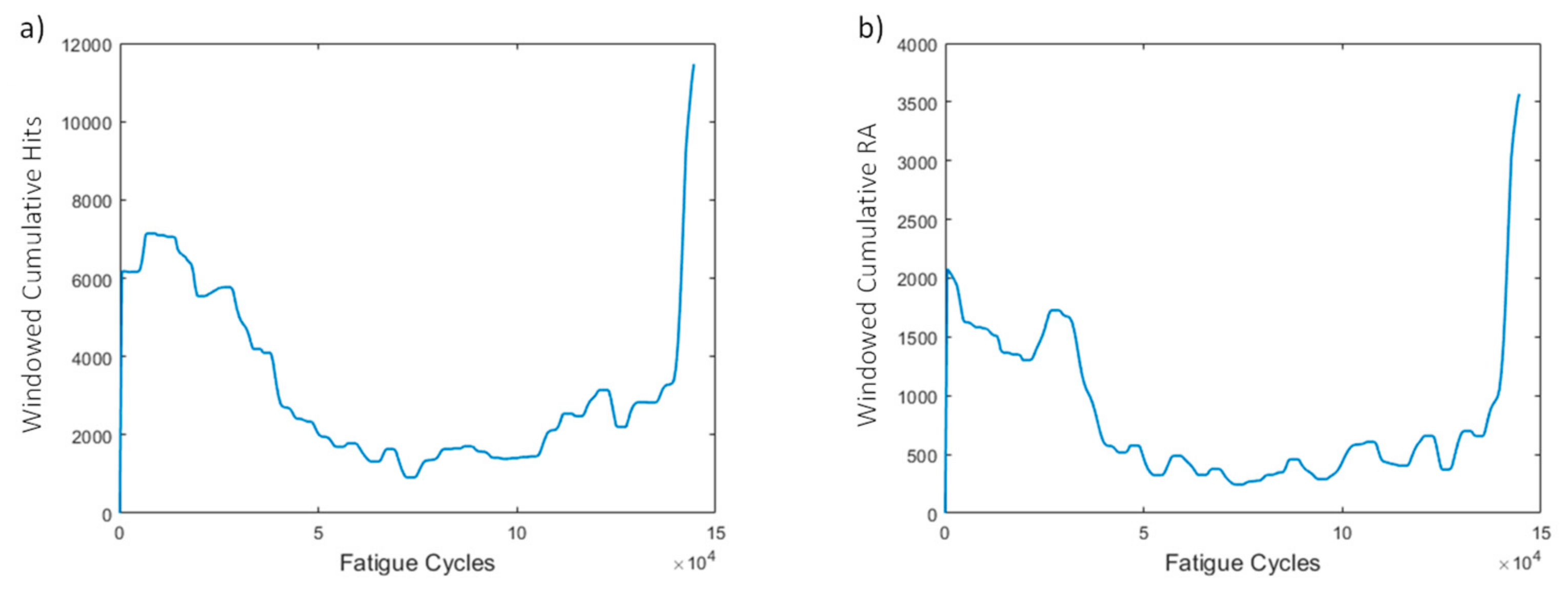
3.3. Acoustic Emission Based HIs
4. Results and Discussion
4.1. Constant Amplitude Fatigue
4.1.1. Strain-Based HIs
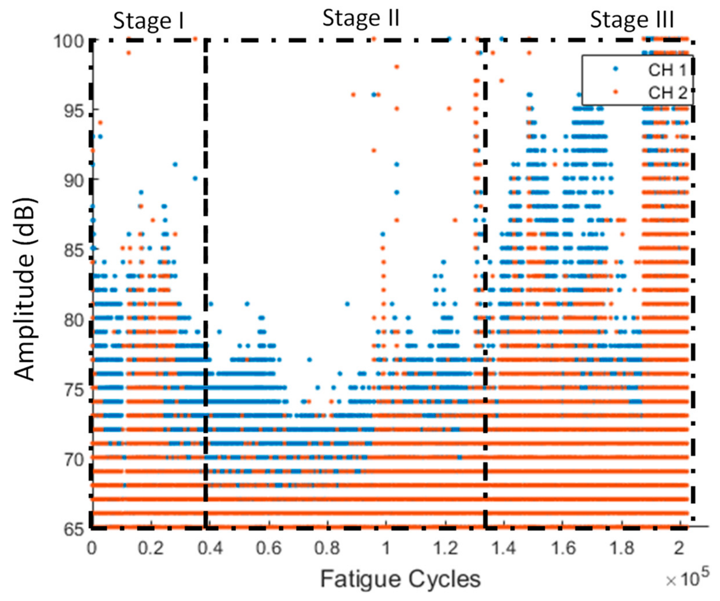
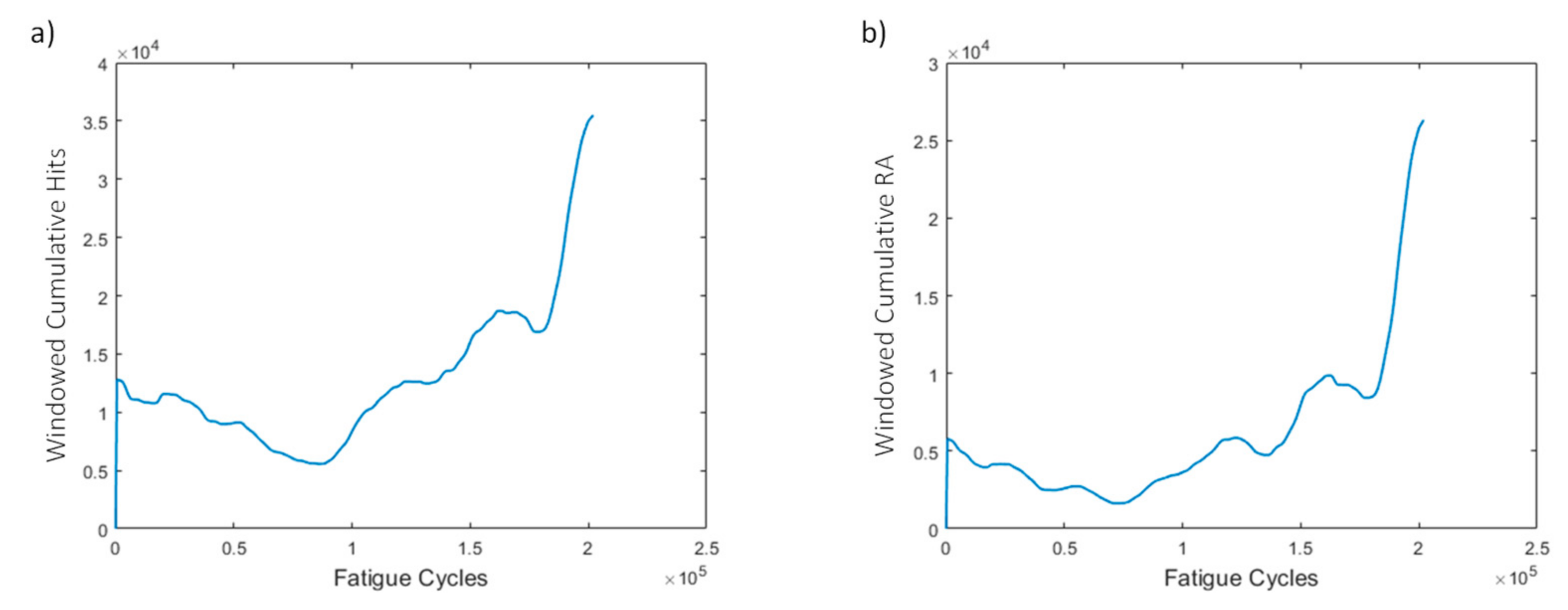
4.1.2. AE-Based HIs
4.2. Variable Amplitude Fatigue
4.2.1. Strain-Based HIs
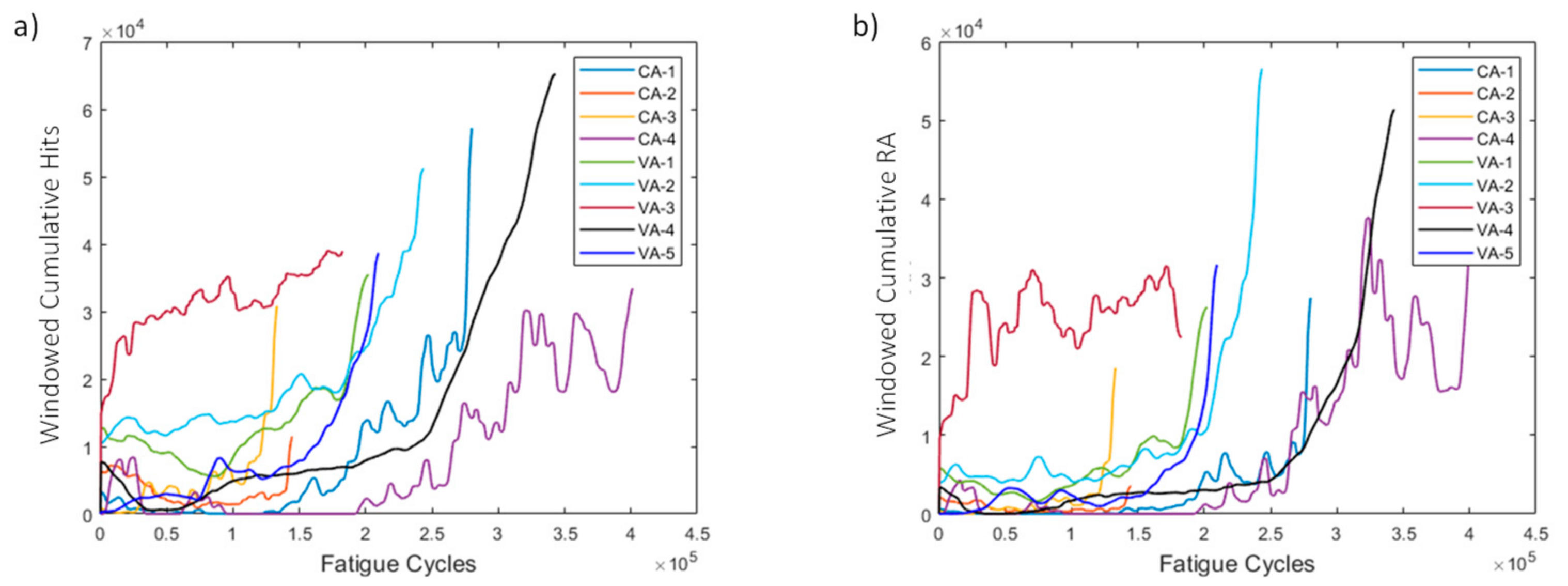
4.2.2. AE Based HIs
4.3. Discussion
5. Conclusions
Author Contributions
Funding
Institutional Review Board Statement
Informed Consent Statement
Data Availability Statement
Acknowledgments
Conflicts of Interest
References
- Kassapoglou, C. Design and Analysis of Composite Structures: With Applications to Aerospace Structures; John Wiley & Sons: Hoboken, NJ, USA, 2013. [Google Scholar]
- Andreades, C.; Meo, M.; Ciampa, F. Fatigue testing and damage evaluation using smart CFRP composites with embedded PZT transducers. Mater. Today Proc. 2021, 34, 260–265. [Google Scholar] [CrossRef]
- Marques, R.; Unel, M.; Yildiz, M.; Suleman, A. Remaining useful life prediction of laminated composite materials using thermoelastic stress analysis. Compos. Struct. 2019, 210, 381–390. [Google Scholar] [CrossRef]
- Loutas, T.; Eleftheroglou, N.; Zarouchas, D. A data-driven probabilistic framework towards the in-situ prognostics of fatigue life of composites based on acoustic emission data. Compos. Struct. 2017, 161, 522–529. [Google Scholar] [CrossRef]
- Eleftheroglou, N.; Loutas, T. Fatigue damage diagnostics and prognostics of composites utilizing structural health monitoring data and stochastic processes. Struct. Health Monit. Int. J. 2016, 15, 473–488. [Google Scholar] [CrossRef]
- Grassia, L.; Iannone, M.; Califano, A.; D’Amore, A. Strain based method for monitoring the health state of composite structures. Compos. Part B Eng. 2019, 176, 107253. [Google Scholar] [CrossRef]
- Milanoski, D.P.; Loutas, T.H. Strain-based health indicators for the structural health monitoring of stiffened composite panels. J. Intell. Mater. Syst. Struct. 2021, 32, 255–266. [Google Scholar] [CrossRef]
- Palaniappan, J.; Ogin, S.; Thorne, A.; Reed, G.; Crocombe, A.; Capell, T.; Tjin, S.; Mohanty, L. Disbond growth detection in composite–composite single-lap joints using chirped FBG sensors. Compos. Sci. Technol. 2008, 68, 2410–2417. [Google Scholar] [CrossRef] [Green Version]
- Kahandawa, G.C.; Epaarachchi, J.; Wang, H.; Lau, K.T. Use of FBG Sensors for SHM in Aerospace Structures. Photonic Sens. 2012, 2, 203–214. [Google Scholar] [CrossRef] [Green Version]
- Takeda, S.-I.; Aoki, Y.; Nagao, Y. Damage monitoring of CFRP stiffened panels under compressive load using FBG sensors. Compos. Struct. 2012, 94, 813–819. [Google Scholar] [CrossRef]
- Sbarufatti, C.; Corbetta, M.; San Millan, J.; Frovel, M.; Stefaniuk, M.; Giglio, M. Model-Assisted Performance Qualification of a Distributed SHM System for Fatigue Crack Detection on a Helicopter Tail Boom. In Proceedings of the 8th European Workshop on Structural Health Monitoring, Bilbao, Spain, 5–8 July 2016. [Google Scholar]
- Sbarufatti, C.; Manes, A.; Giglio, M. Performance optimization of a diagnostic system based upon a simulated strain field for fatigue damage characterization. Mech. Syst. Signal Process. 2013, 40, 667–690. [Google Scholar] [CrossRef]
- Guemes, A.; Sierra, J.; Rodellar, J.; Mujica, L. A robust procedure for Damage detection from strain measurements based on Principal Component Analysis. In Key Engineering Materials; Trans Tech Publications Ltd.: Freienbach, Switzerland, 2013; pp. 128–138. [Google Scholar]
- Güemes, A.; Fernández-López, A.; Díaz-Maroto, P.F.; Lozano, A.; Sierra-Perez, J. Structural Health Monitoring in Composite Structures by Fiber-Optic Sensors. Sensors 2018, 18, 1094. [Google Scholar] [CrossRef] [PubMed] [Green Version]
- Saeedifar, M.; Zarouchas, D. Damage characterization of laminated composites using acoustic emission: A review. Compos. Part B Eng. 2020, 195, 108039. [Google Scholar] [CrossRef]
- Zhou, W.; Lv, Z.-H.; Li, Z.-Y.; Song, X. Acoustic emission response and micro-deformation behavior for compressive buckling failure of multi-delaminated composites. J. Strain Anal. Eng. Des. 2016, 51, 397–407. [Google Scholar] [CrossRef]
- Carmi, R.; Wisner, B.; Vanniamparambil, P.A.; Cuadra, J.A.; Bussiba, A.; Kontsos, A. Progressive Failure Monitoring of Fiber-Reinforced Metal Laminate Composites Using a Nondestructive Approach. J. Nondestruct. Eval. Diagn. Progn. Eng. Syst. 2019, 2, 021006. [Google Scholar] [CrossRef]
- Liu, Y.; Mohanty, S.; Chattopadhyay, A. A Gaussian process based prognostics framework for composite structures. In Proceedings of the Modeling, Signal Processing, and Control for Smart Structures 2009, San Diego, CA, USA, 11–12 March 2009; International Society for Optics and Photonics: Bellingham, WA, USA, 2009. [Google Scholar]
- Yu, F.-M.; Okabe, Y.; Wu, Q.; Shigeta, N. A novel method of identifying damage types in carbon fiber-reinforced plastic cross-ply laminates based on acoustic emission detection using a fiber-optic sensor. Compos. Sci. Technol. 2016, 135, 116–122. [Google Scholar] [CrossRef]
- Perez, I.M.; Cui, H.; Udd, E. Acoustic emission detection using fiber Bragg gratings. In Proceedings of the Smart Structures and Materials 2001: Sensory Phenomena and Measurement Instrumentation for Smart Structures and Materials, Newport Beach, CA, USA, 5–6 March 2001; International Society for Optics and Photonics: Bellingham, WA, USA, 2001. [Google Scholar]
- Tsuda, H.; Sato, E.; Nakajima, T.; Nakamura, H.; Arakawa, T.; Shiono, H.; Minato, M.; Kurabayashi, H.; Sato, A. Acoustic emission measurement using a strain-insensitive fiber Bragg grating sensor under varying load conditions. Opt. Lett. 2009, 34, 2942–2944. [Google Scholar] [CrossRef]
- Broer, A.; Galanopoulos, G.; Benedictus, R.; Loutas, T.; Zarouchas, D. Fusion-based damage diagnostics for stiffened composite panels. Struct. Health Monit. 2021, in press. [Google Scholar] [CrossRef]
- Broer, A.A.R.; Galanopoulos, G.; Zarouchas, D.; Loutas, T.; Benedictus, R. Damage Diagnostics of a Composite Single-Stiffener Panel Under Fatigue Loading Utilizing SHM Data Fusion. In Proceedings of the European Workshop on Structural Health Monitoring, Palermo, Italy, 6–9 July 2020; Springer: Berlin/Heidelberg, Germany, 2020. [Google Scholar]
- Loutas, T.; Eleftheroglou, N.; Georgoulas, G.; Loukopoulos, P.; Mba, D.; Bennett, I. Valve Failure Prognostics in Reciprocating Compressors Utilizing Temperature Measurements, PCA-Based Data Fusion, and Probabilistic Algorithms. IEEE Trans. Ind. Electron. 2020, 67, 5022–5029. [Google Scholar] [CrossRef]
- Eleftheroglou, N.; Zarouchas, D.; Loutas, T.; Alderliesten, R.; Benedictus, R. Structural health monitoring data fusion for in-situ life prognosis of composite structures. Reliab. Eng. Syst. Saf. 2018, 178, 40–54. [Google Scholar] [CrossRef] [Green Version]
- Hu, C.; Youn, B.D.; Wang, P.; Yoon, J.T. An ensemble approach for robust data-driven prognostics. In Proceedings of the International Design Engineering Technical Conferences and Computers and Information in Engineering Conference, Chicago, IL, USA, 12–15 August 2012; American Society of Mechanical Engineers: New York, NY, USA, 2012. [Google Scholar]
- Wen, P.; Zhao, S.; Chen, S.; Li, Y. A generalized remaining useful life prediction method for complex systems based on composite health indicator. Reliab. Eng. Syst. Saf. 2021, 205, 107241. [Google Scholar] [CrossRef]
- Eleftheroglou, N.; Zarouchas, D.; Loutas, T.; Alderliesten, R.C.; Benedictus, R. Online remaining fatigue life prognosis for composite materials based on strain data and stochastic modeling. In Key Engineering Materials; Trans Tech Publications Ltd.: Freienbach, Switzerland, 2016. [Google Scholar]
- Milanoski, D.; Galanopoulos, G.; Broer, A.; Zarouchas, D.; Loutas, T. A Strain-Based Health Indicator for the SHM of Skin-to-Stringer Disbond Growth of Composite Stiffened Panels in Fatigue. In Proceedings of the European Workshop on Structural Health Monitoring, Palermo, Italy, 6–9 July 2020; Springer: Berlin/Heidelberg, Germany, 2020. [Google Scholar]
- Loukopoulos, P.; Zolkiewski, G.; Bennett, I.; Sampath, S.; Pilidis, P.; Duan, F.; Sattar, T.; Mba, D. Reciprocating compressor prognostics of an instantaneous failure mode utilising temperature only measurements. Appl. Acoust. 2019, 147, 77–86. [Google Scholar] [CrossRef]
- Zhang, Z.; Wang, Y.; Wang, K. Intelligent fault diagnosis and prognosis approach for rotating machinery integrating wavelet transform, principal component analysis, and artificial neural networks. Int. J. Adv. Manuf. Technol. 2013, 68, 763–773. [Google Scholar] [CrossRef]
- Shahid, N.; Ghosh, A. TrajecNets: Online Failure Evolution Analysis in 2D Space; United Technologies Research Center, Penrose Wharf Business Center: Cork, Ireland, 2019. [Google Scholar]
- Inaudi, D.; Glisic, B. Development of distributed strain and temperature sensing cables. In Proceedings of the 17th International Conference on Optical Fibre Sensors, Bruges, Belgium, 23–27 May 2005; International Society for Optics and Photonics: Bellingham, WA, USA, 2005. [Google Scholar]
- Sierra-Pérez, J.; Güemes, A.; Mujica, L.; Ruiz, M. Damage detection in composite materials structures under variable loads conditions by using fiber Bragg gratings and principal component analysis, involving new unfolding and scaling methods. J. Intell. Mater. Syst. Struct. 2015, 26, 1346–1359. [Google Scholar] [CrossRef]
- Ahmed, M.; Gu, F.; Ball, A. Fault detection of reciprocating compressors using a model from principles component analysis of vibrations. In Proceedings of the Journal of Physics: Conference Series, Varenna, Italy, 27–31 August 2012; IOP Publishing: Bristol, UK, 2012. [Google Scholar]
- Milanoski, D.P.; Loutas, T.H. Strain-based damage assessment of stiffened composite panels for structural health monitoring purposes. In Proceedings of the 9th Thematic Conference on Smart Structures and Materials, Paris, France, 8–11 July 2019. [Google Scholar]
- Javed, K.; Gouriveau, R.; Zerhouni, N.; Nectoux, P. Enabling health monitoring approach based on vibration data for accurate prognostics. IEEE Trans. Ind. Electron. 2014, 62, 647–656. [Google Scholar] [CrossRef] [Green Version]
- Abràmoff, M.D.; Magalhães, P.J.; Ram, S.J. Image processing with ImageJ. Biophotonics Int. 2004, 11, 36–42. [Google Scholar]
- Holmes, C.; Godfrey, M.; Bull, D.J.; Dulieu-Barton, J. Real-time through-thickness and in-plane strain measurement in carbon fibre reinforced polymer composites using planar optical Bragg gratings. Opt. Lasers Eng. 2020, 133, 106111. [Google Scholar] [CrossRef]

| Specimen # | Impact Location/Disbond | Impact Energy/Disbond Size | Load | # of Cycles to Failure | |
|---|---|---|---|---|---|
| Min. | Max. | ||||
| CA-1 | Skin | 10 J | −6.5 kN | −65 kN | 280,098 |
| CA-2 | Stiffener foot | 10 J | −6.5 kN | −65 kN | 144,969 |
| CA-3 | Stiffener foot | 10 J | −6.5 kN | −65 kN | 133,281 |
| CA-4 | Stiffener foot | 30 mm | −5.0 kN −6.0 kN 1 | −50 kN −60 kN 1 | 438,000 |
| Specimen # | Impact Location/Disbond | Impact Energy/Disbond Size | Load | # of Cycles | |
|---|---|---|---|---|---|
| Min. | Max. | ||||
| VA-1 | Stiffener foot | 7.4 J | −4.0 kN −4.5 kN −5.0 kN −5.5 kN −6.0 kN | −40 kN −45 kN −50 kN −55 kN −60 kN | 10,000 80,000 30,000 70,000 12,300 202,300 |
| VA-2 | Stiffener foot | 10 J | −4.0 kN −4.5 kN −5.0 kN −5.5 kN | −40 kN −45 kN −50 kN −55 kN | 10,000 80,000 90,000 63,000 243,000 |
| VA-3 | Stiffener foot | 10 J | −4.0 kN −4.5 kN −5.0 kN | −40 kN −45 kN −50 kN | 10,000 177,000 30,000 217,000 |
| VA-4 | Stiffener foot | 30 mm | −3.5 kN −3.9 kN −4.5 kN −5.0 kN −5.5 kN −6.0 kN | −35 kN −39 kN −45 kN −50 kN −55 kN −60 kN | 10,000 10,000 10,000 170,000 85,000 60,000 345,000 |
| VA-5 | Stiffener foot | 7.37 J | −4.0 kN −4.5 kN −5.0 kN −5.5 kN −6.0 kN | −40 kN −45 kN −50 kN −55 kN −60 kN | 20,000 75,000 25,000 62,000 60,000 242,000 |
Publisher’s Note: MDPI stays neutral with regard to jurisdictional claims in published maps and institutional affiliations. |
© 2021 by the authors. Licensee MDPI, Basel, Switzerland. This article is an open access article distributed under the terms and conditions of the Creative Commons Attribution (CC BY) license (https://creativecommons.org/licenses/by/4.0/).
Share and Cite
Galanopoulos, G.; Milanoski, D.; Broer, A.; Zarouchas, D.; Loutas, T. Health Monitoring of Aerospace Structures Utilizing Novel Health Indicators Extracted from Complex Strain and Acoustic Emission Data. Sensors 2021, 21, 5701. https://doi.org/10.3390/s21175701
Galanopoulos G, Milanoski D, Broer A, Zarouchas D, Loutas T. Health Monitoring of Aerospace Structures Utilizing Novel Health Indicators Extracted from Complex Strain and Acoustic Emission Data. Sensors. 2021; 21(17):5701. https://doi.org/10.3390/s21175701
Chicago/Turabian StyleGalanopoulos, Georgios, Dimitrios Milanoski, Agnes Broer, Dimitrios Zarouchas, and Theodoros Loutas. 2021. "Health Monitoring of Aerospace Structures Utilizing Novel Health Indicators Extracted from Complex Strain and Acoustic Emission Data" Sensors 21, no. 17: 5701. https://doi.org/10.3390/s21175701
APA StyleGalanopoulos, G., Milanoski, D., Broer, A., Zarouchas, D., & Loutas, T. (2021). Health Monitoring of Aerospace Structures Utilizing Novel Health Indicators Extracted from Complex Strain and Acoustic Emission Data. Sensors, 21(17), 5701. https://doi.org/10.3390/s21175701