
Surface Roughness Effects on Self-Interacting and Mutually Interacting Rayleigh Waves


Abstract
:1. Introduction
2. Materials and Methods
2.1. Relative Nonlinearity Parameter
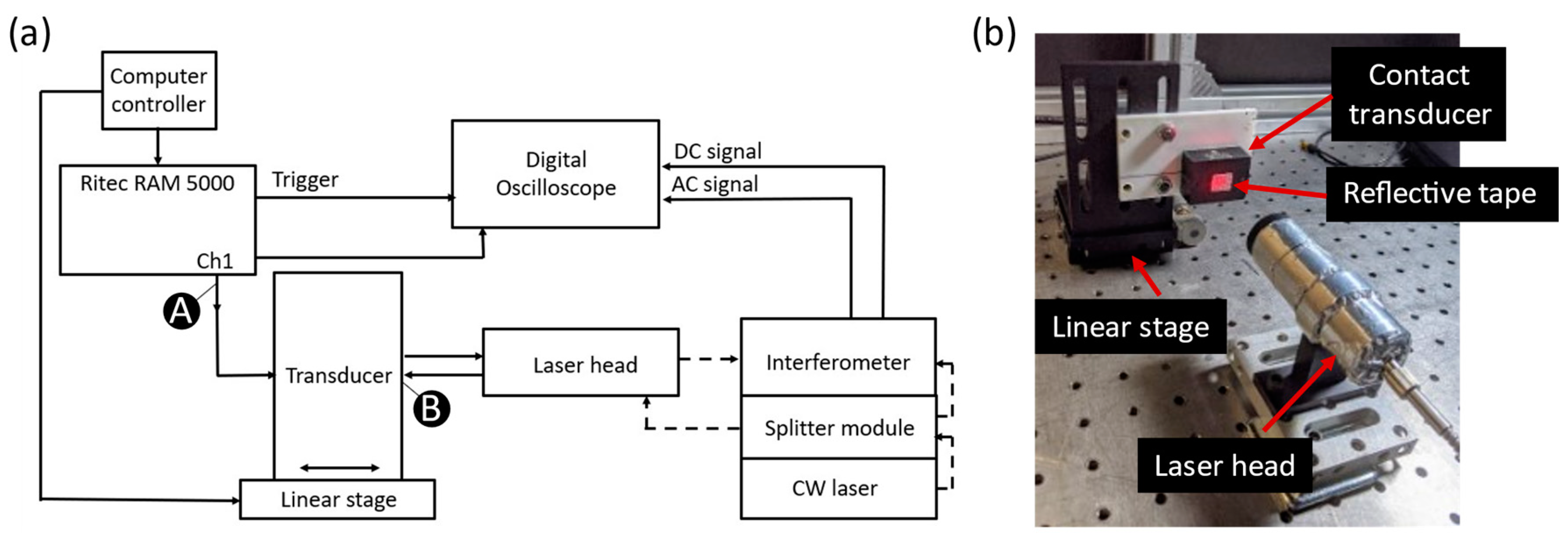
2.2. Self-Interaction of Rayleigh Waves
- Point A—amplifier output monitoring point
- Point B—surface of the transducer, measured by laser interferometer
- Point C—surface of the wedge, measured by laser interferometer
- Point D—surface of the specimen, measured by laser interferometer.
2.3. Mutual Interaction of Rayleigh Waves
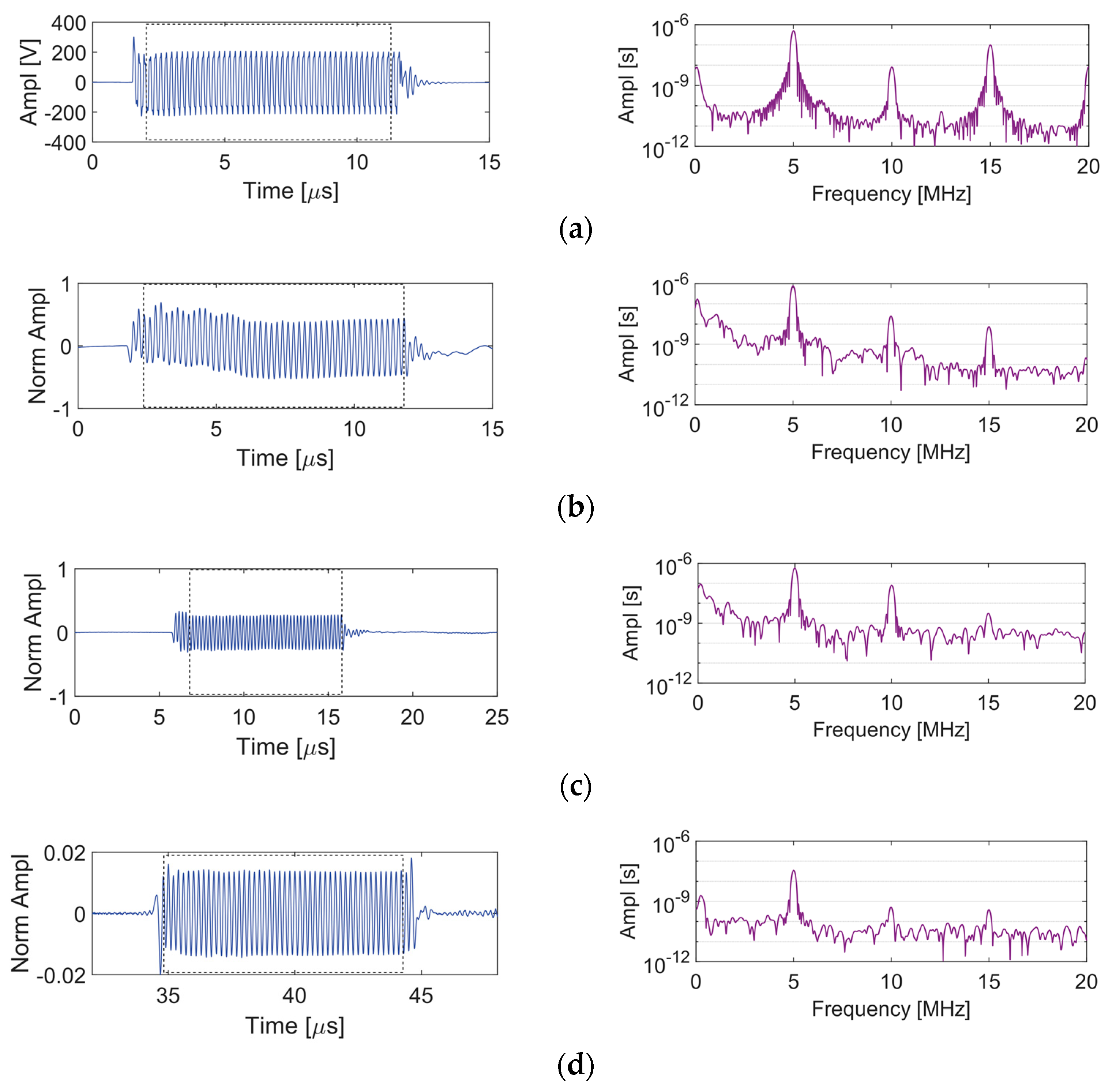
2.4. Signal Processing
3. Results
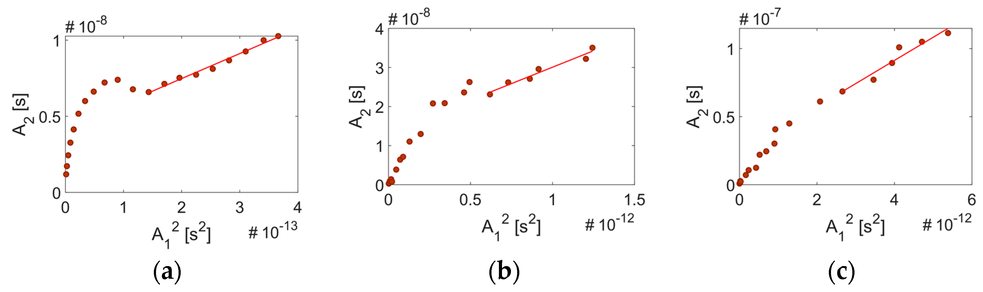
3.1. Sensing System Nonlinearity
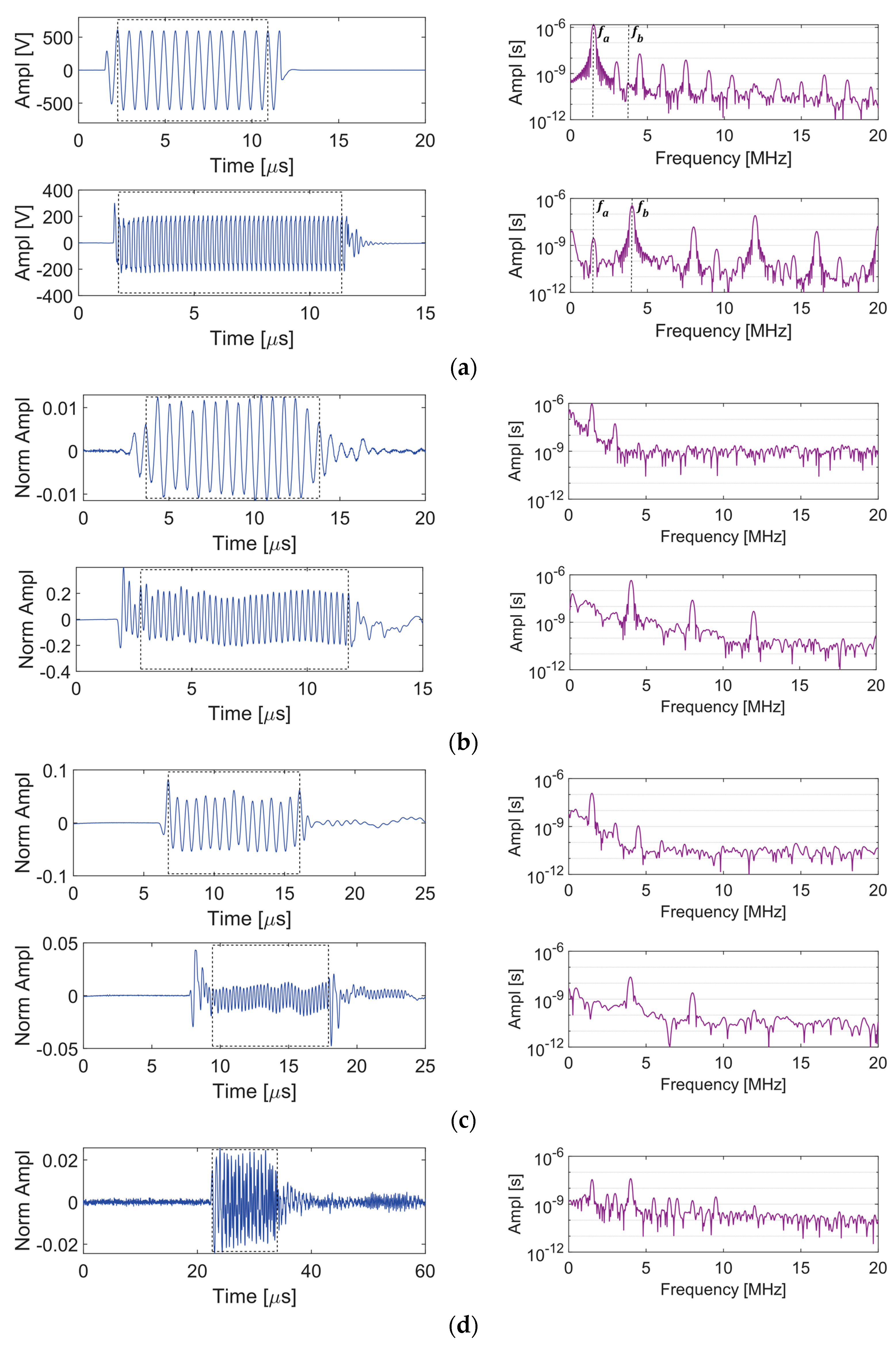
3.2. Nonlinear Rayleigh Wave Mixing Methods
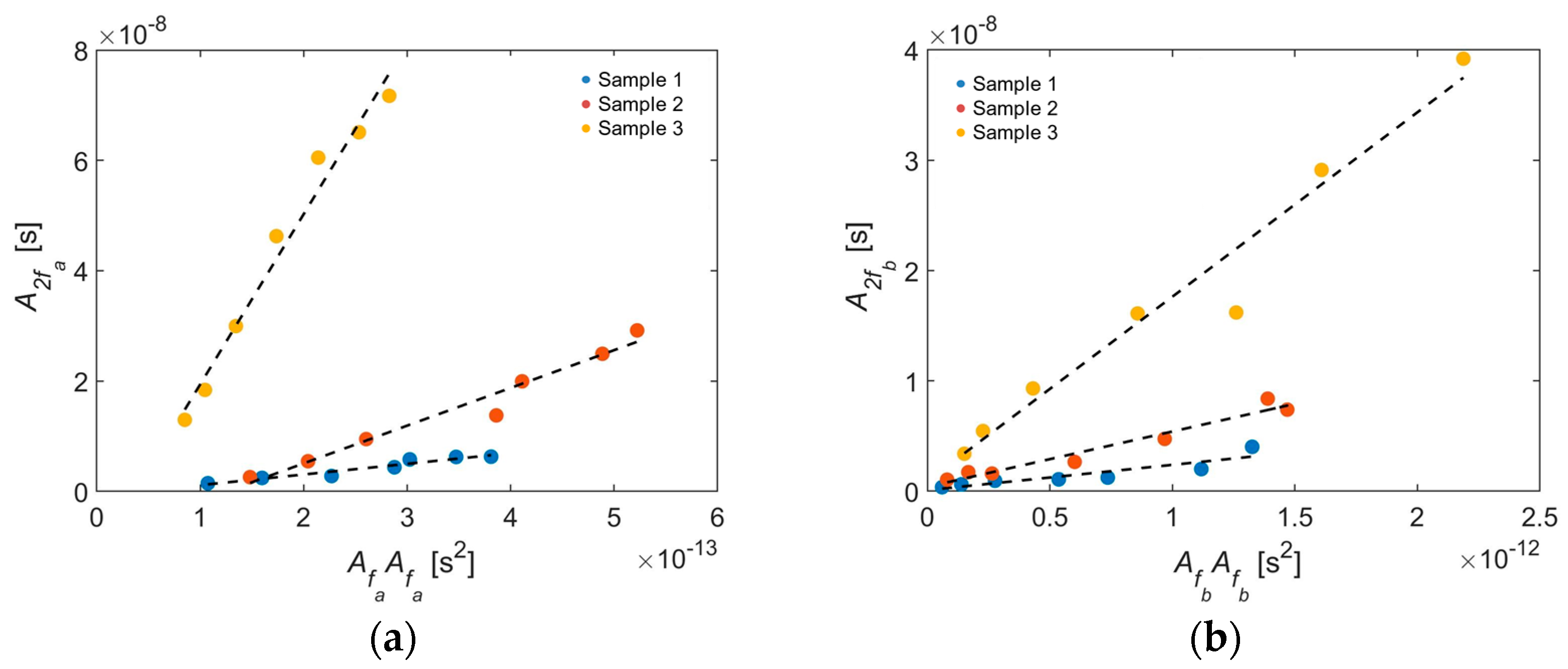
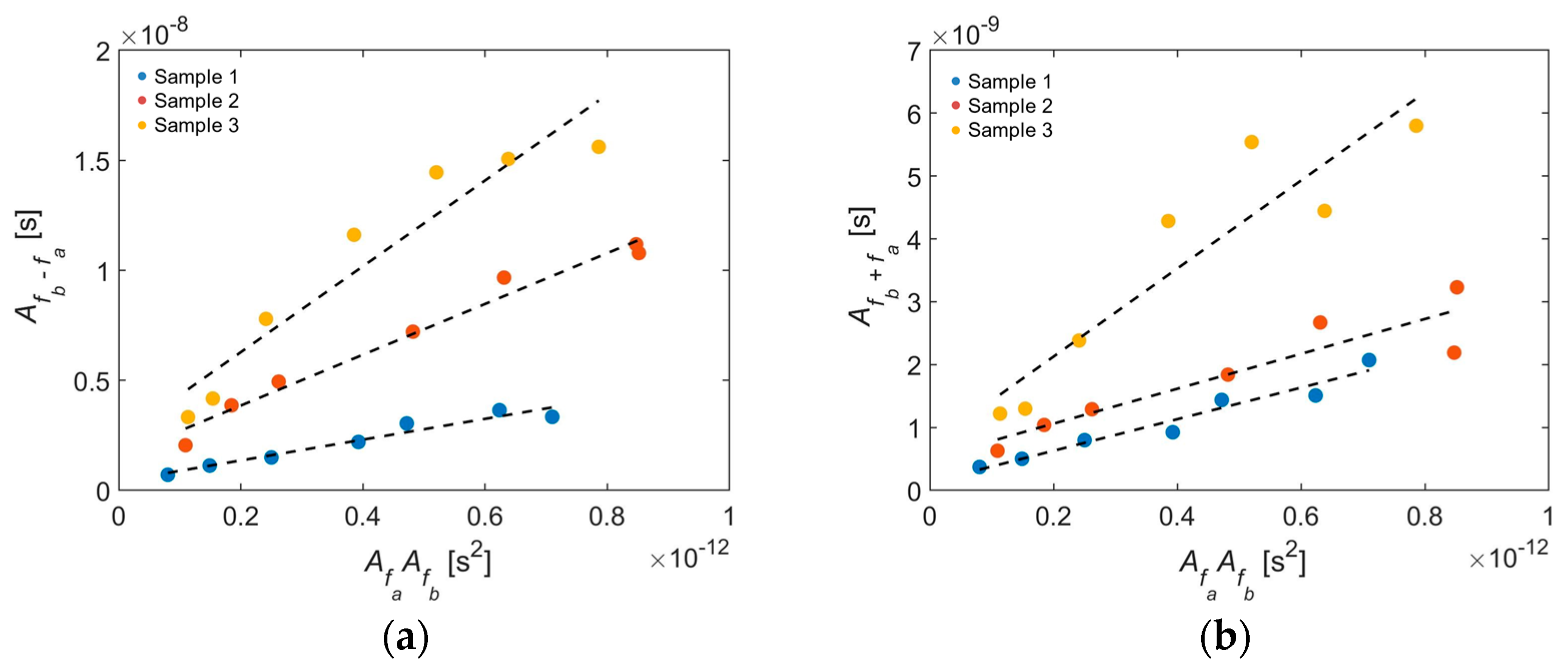
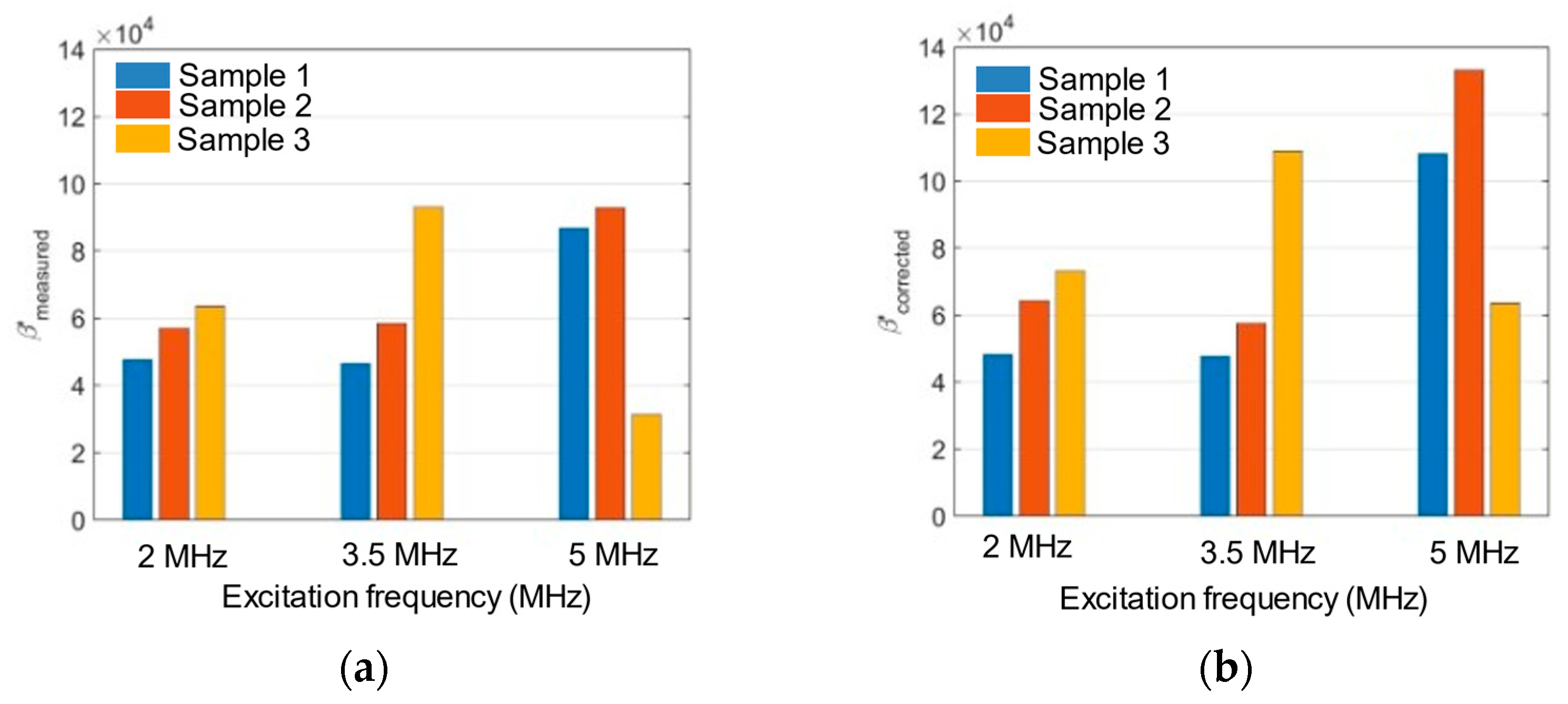
3.3. Surface Roughness Effects on Rayleigh Wave Interactions
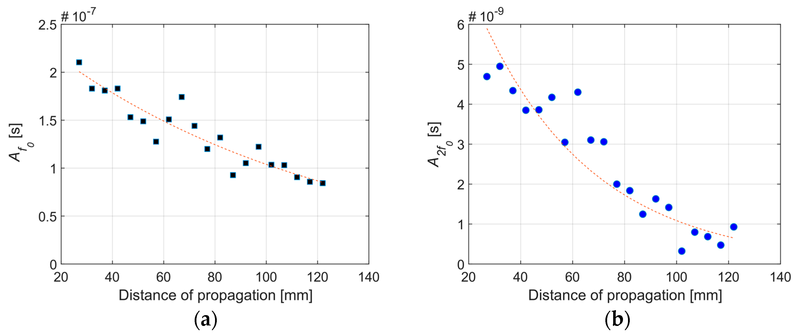
3.4. Effect of Attenuation
4. Discussion
5. Conclusions
Supplementary Materials
Author Contributions
Funding
Institutional Review Board Statement
Informed Consent Statement
Data Availability Statement
Conflicts of Interest
References
- Staszewski, W.J. Structural Health Monitoring Using Guided Ultrasonic Waves. In Advances in Smart Technologies in Structural Engineering; Springer: Berlin/Heidelberg, Germany, 2004; pp. 117–162. [Google Scholar]
- Hirsekorn, S. The scattering of ultrasonic waves by polycrystals. J. Acoust. Soc. Am. 1982, 72, 1021–1031. [Google Scholar] [CrossRef]
- Badidi Bouda, A. Grain size influence on ultrasonic velocities and attenuation. NDT E Int. 2003, 36, 1–5. [Google Scholar] [CrossRef]
- Papadakis, E.P. Rayleigh and Stochastic Scattering of Ultrasonic Waves in Steel. J. Appl. Phys. 1963, 34, 265–269. [Google Scholar] [CrossRef]
- Moghanizadeh, A.; Farzi, A. Effect of heat treatment on an AISI 304 austenitic stainless steel evaluated by the ultrasonic attenuation coefficient. Mater. Test. 2016, 58, 448–452. [Google Scholar] [CrossRef]
- Laux, D.; Cros, B.; Despaux, G.; Baron, D. Ultrasonic study of UO2: Effects of porosity and grain size on ultrasonic attenuation and velocities. J. Nucl. Mater. 2002, 300, 192–197. [Google Scholar] [CrossRef]
- Tardy, F.; Nadal, M.H.; Gondard, C.; Paradis, L.; Guy, P.; Baboux, J.C. Microstructural Characterization of Materials by a Rayleigh Wave Analysis. In Review of Progress in Quantitative Nondestructive Evaluation; Springer: Boston, MA, USA, 1997; pp. 1399–1405. [Google Scholar]
- Wang, M.; Bu, Y.; Dai, Z.; Zeng, S. Characterization of Grain Size in 316L Stainless Steel Using the Attenuation of Rayleigh Wave Measured by Air-Coupled Transducer. Materials 2021, 14, 1901. [Google Scholar] [CrossRef]
- Chakrapani, S.K.; Bond, L.J. Rayleigh Wave Nondestructive Evaluation for Defect Detection and Materials Characterization. In Nondestructive Evaluation of Materials; ASM International: Russell Township, OH, USA, 2018; Volume 17, pp. 266–282. [Google Scholar]
- Nagy, P.B. Fatigue damage assessment by nonlinear ultrasonic materials characterization. Ultrasonics 1998, 36, 375–381. [Google Scholar] [CrossRef]
- Walker, S.V.; Kim, J.Y.; Qu, J.; Jacobs, L.J. Fatigue damage evaluation in A36 steel using nonlinear Rayleigh surface waves. NDT E Int. 2012, 48, 10–15. [Google Scholar] [CrossRef]
- Liu, M.; Kim, J.Y.; Jacobs, L.; Qu, J. Experimental study of nonlinear Rayleigh wave propagation in shot-peened aluminum plates Feasibility of measuring residual stress. NDT E Int. 2011, 44, 67–74. [Google Scholar] [CrossRef]
- Thiele, S.; Kim, J.-Y.; Qu, J.; Jacobs, L.J. Air-coupled detection of nonlinear Rayleigh surface waves to assess material nonlinearity. Ultrasonics 2014, 54, 1470–1475. [Google Scholar] [CrossRef]
- Matlack, K.H.; Bradley, H.A.; Thiele, S.; Kim, J.-Y.; Wall, J.J.; Jung, H.J.; Qu, J.; Jacobs, L.J. Nonlinear ultrasonic characterization of precipitation in 17-4PH stainless steel. NDT E Int. 2015, 71, 8–15. [Google Scholar] [CrossRef] [Green Version]
- Gutiérrez-Vargas, G.; Ruiz, A.; Kim, J.-Y.; Jacobs, L.J. Characterization of thermal embrittlement in 2507 super duplex stainless steel using nonlinear acoustic effects. NDT E Int. 2018, 94, 101–108. [Google Scholar] [CrossRef]
- Jun, J.; Seo, H.; Jhang, K.Y. Nondestructive evaluation of thermal aging in Al6061 alloy by measuring acoustic nonlinearity of laser-generated surface acoustic waves. Metals 2020, 10, 38. [Google Scholar] [CrossRef] [Green Version]
- Doerr, C.; Kim, J.Y.; Singh, P.; Wall, J.J.; Jacobs, L.J. Evaluation of sensitization in stainless steel 304 and 304L using nonlinear Rayleigh waves. NDT E Int. 2017, 88, 17–23. [Google Scholar] [CrossRef]
- Zeitvogel, D.T.; Matlack, K.H.; Kim, J.-Y.; Jacobs, L.J.; Singh, P.M.; Qu, J. Characterization of stress corrosion cracking in carbon steel using nonlinear Rayleigh surface waves. NDT E Int. 2014, 62, 144–152. [Google Scholar] [CrossRef]
- Ghafoor, I.; Tse, P.W.; Rostami, J.; Ng, K.-M. Non-Contact Inspection of Railhead via Laser-Generated Rayleigh Waves and an Enhanced Matching Pursuit to Assist Detection of Surface and Subsurface Defects. Sensors 2021, 21, 2994. [Google Scholar] [CrossRef]
- Li, K.; Jing, S.; Yu, J.; Zhang, B. Complex Rayleigh Waves in Nonhomogeneous Magneto-Electro-Elastic Half-Spaces. Materials 2021, 14, 1011. [Google Scholar] [CrossRef]
- Song, H.; Hong, J.; Choi, H.; Min, J. Concrete Delamination Depth Estimation Using a Noncontact MEMS Ultrasonic Sensor Array and an Optimization Approach. Appl. Sci. 2021, 11, 592. [Google Scholar] [CrossRef]
- Li, H.; Pan, Q.; Zhang, X.; An, Z. An Approach to Size Sub-Wavelength Surface Crack Measurements Using Rayleigh Waves Based on Laser Ultrasounds. Sensors 2020, 20, 5077. [Google Scholar] [CrossRef]
- Sarris, G.; Haslinger, S.G.; Huthwaite, P.; Nagy, P.B.; Lowe, M.J.S. Attenuation of Rayleigh waves due to surface roughness. J. Acoust. Soc. Am. 2021, 149, 4298–4308. [Google Scholar] [CrossRef] [PubMed]
- Krylov, V.; Smirnova, Z. Experimental study of the dispersion of a Rayleigh wave on a rough surface. Sov. Phys. Acoust. 1990, 36, 583–585. [Google Scholar]
- Maradudin, A.A.; Mills, D.L. The attenuation of Rayleigh surface waves by surface roughness. Ann. Phys. 1976, 100, 262–309. [Google Scholar] [CrossRef]
- Huang, X.; Maradudin, A.A. Propagation of surface acoustic waves across random gratings. Phys. Rev. B 1987, 36, 7827–7839. [Google Scholar] [CrossRef] [PubMed]
- Eguiluz, A.G.; Maradudin, A.A. Frequency shift and attenuation length of a Rayleigh wave due to surface roughness. Phys. Rev. B 1983, 28, 728–747. [Google Scholar] [CrossRef]
- Urazakov, E.I.; Fal’kovskii, L.A. Propagation of a Rayleigh wave along a rough surface. JETP 1973, 36, 1214–1216. [Google Scholar]
- Steg, R.G.; Klemens, P.G. Scattering of Rayleigh waves by surface defects. J. Appl. Phys. 1974, 45, 23–29. [Google Scholar] [CrossRef]
- De Billy, M.; Quentin, G.; Baron, E. Attenuation measurements of an ultrasonic Rayleigh wave propagating along rough surfaces. J. Appl. Phys. 1987, 61, 2140–2145. [Google Scholar] [CrossRef]
- Sinclair, R. Velocity Dispersion of Rayleigh Waves Propagating along Rough Surfaces. J. Acoust. Soc. Am. 1971, 50, 841–845. [Google Scholar] [CrossRef]
- Ruiz, A.; Nagy, P.B. Laser-ultrasonic surface wave dispersion measurements on surface-treated metals. Ultrasonics 2004, 42, 665–669. [Google Scholar] [CrossRef]
- Ruiz, A.; Nagy, P.B. SAW dispersion measurements for ultrasonic characterization of surface-treated metals. Instr. Meas. Metrol. 2003, 3, 59. [Google Scholar]
- Cantrell, J. Fundamentals and Applications of Nonlinear Ultrasonic Nondestructive Evaluation. In Ultrasonic Nondestructive Evaluation; CRC Press: Boca Raton, FL, USA, 2003. [Google Scholar]
- Nečas, D.; Klapetek, P. Gwyddion: An open-source software for SPM data analysis. Open Phys. 2012, 10, 181–188. [Google Scholar] [CrossRef]
- Deltombe, R.; Kubiak, K.J.; Bigerelle, M. How to select the most relevant 3D roughness parameters of a surface. Scanning 2014, 36, 150–160. [Google Scholar] [CrossRef] [PubMed] [Green Version]
- Wang, Z.; Cui, X.; Ma, H.; Kang, Y.; Deng, Z. Effect of Surface Roughness on Ultrasonic Testing of Back-Surface Micro-Cracks. Appl. Sci. 2018, 8, 1233. [Google Scholar] [CrossRef] [Green Version]
- Torello, D.; Thiele, S.; Matlack, K.H.; Kim, J.-Y.; Qu, J.; Jacobs, L.J. Diffraction, attenuation, and source corrections for nonlinear Rayleigh wave ultrasonic measurements. Ultrasonics 2015, 56, 417–426. [Google Scholar] [CrossRef] [Green Version]
- Jhang, K.-Y.; Lissenden, C.J.; Solodov, I.; Ohara, Y.; Gusev, V. Measurement of Nonlinear Ultrasonic Characteristics; Springer Series in Measurement Science and Technology; Springer: Singapore, 2020; ISBN 978-981-15-1460-9. [Google Scholar]
- Hikata, A.; Elbaum, C. Generation of Ultrasonic Second and Third Harmonics Due to Dislocations. I. Phys. Rev. 1966, 144, 469–477. [Google Scholar] [CrossRef]


| Sample | 3D Surface Profile | 1D Surface Profile |
|---|---|---|
| 1 Smooth | 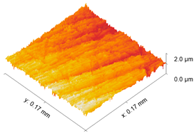 | 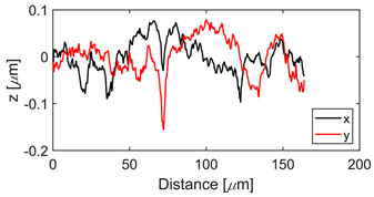 |
| 2 Moderate | 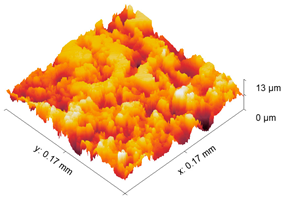 | 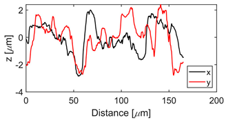 |
| 3 Rough | 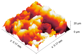 |  |
| Sample | Linear Roughness Parameters (ISO 4287): x-Direction | |||||
|---|---|---|---|---|---|---|
| m | m | m | ||||
| 1 (Smooth) | 0.027 | 0.034 | 0.173 | |||
| 2 (Moderate) | 0.872 | 1.081 | 4.849 | |||
| 3 (Rough) | 3.992 | 4.649 | 16.403 | |||
| Sample | Linear Roughness Parameters (ISO 4287): y-Direction | |||||
| m | m | m | ||||
| 1 (Smooth) | 0.033 | 0.040 | 0.234 | |||
| 2 (Moderate) | 1.034 | 1.304 | 5.178 | |||
| 3 (Rough) | 3.410 | 3.923 | 13.365 | |||
| Sample | Areal Roughness Parameters (ISO 25178-2) | |||||
| m | m | m | Sdq | |||
| 1 (Smooth) | 0.0831 | 0.105 | 0.865 | 0.220 | ||
| 2 (Moderate) | 1.642 | 1.993 | 12.94 | 1.852 | ||
| 3 (Rough) | 4.349 | 5.118 | 20.450 | 2.832 | ||
| Secondary Frequency (MHz) | Relative Nonlinearity Parameter | Roughness Magnification Factor | |||
|---|---|---|---|---|---|
| Sample 1 Smooth | Sample 2 Moderate | Sample 3 Rough | Sample 2/1 | Sample 3/1 | |
| fb−a = 2.5 | 4725 | 11,545 | 19,514 | 2.44 | 4.13 |
| f2a = 3.0 | 19,301 | 33,675 | 308,435 | 1.74 | 16.0 |
| fb+a = 5.5 | 2509 | 2774 | 7003 | 1.10 | 2.79 |
| f2b = 8.0 | 2298 | 5015 | 16,717 | 2.18 | 7.27 |
| Sample | Roughness | fo = 2.0 MHz | fo = 3.5 MHz | fo = 5.0 MHz | |
|---|---|---|---|---|---|
| 1 | Smooth | fo 2fo | 2.3 5.3 | 4.9 11.0 | 5.3 22.0 |
| 2 | Moderate | fo 2fo | 6.4 19.0 | 15.4 30.8 | 19.0 57.2 |
| 3 | Rough | fo 2fo | 11.0 29.3 | 23.0 54.1 | 29.3 99.6 |
| Sample | Roughness | fo = 2.0 MHz | fo = 3.5 MHz | fo = 5.0 MHz |
|---|---|---|---|---|
| 1 | Smooth | 1.0141 | 1.0242 | 1.2453 |
| 2 | Moderate | 1.1290 | 0.9841 | 1.4327 |
| 3 | Rough | 1.1531 | 1.1707 | 2.0347 |
Publisher’s Note: MDPI stays neutral with regard to jurisdictional claims in published maps and institutional affiliations. |
© 2021 by the authors. Licensee MDPI, Basel, Switzerland. This article is an open access article distributed under the terms and conditions of the Creative Commons Attribution (CC BY) license (https://creativecommons.org/licenses/by/4.0/).
Share and Cite
Bakre, C.; Lissenden, C.J. Surface Roughness Effects on Self-Interacting and Mutually Interacting Rayleigh Waves. Sensors 2021, 21, 5495. https://doi.org/10.3390/s21165495
Bakre C, Lissenden CJ. Surface Roughness Effects on Self-Interacting and Mutually Interacting Rayleigh Waves. Sensors. 2021; 21(16):5495. https://doi.org/10.3390/s21165495
Chicago/Turabian StyleBakre, Chaitanya, and Cliff J. Lissenden. 2021. "Surface Roughness Effects on Self-Interacting and Mutually Interacting Rayleigh Waves" Sensors 21, no. 16: 5495. https://doi.org/10.3390/s21165495
APA StyleBakre, C., & Lissenden, C. J. (2021). Surface Roughness Effects on Self-Interacting and Mutually Interacting Rayleigh Waves. Sensors, 21(16), 5495. https://doi.org/10.3390/s21165495