1. Introduction
Air quality in cities and suburban areas is a crucial and emerging problem for governments. Among various air pollutants, airborne particulate matter (PM) with diameters less than 10 micrometers (PM
10) and less than 2.5 micrometers (PM
2.5) are the most common pollutants in Polish cities. PM is a complex mixture of extremely small particles and liquid droplets made up of acids, organic chemicals, metal, soil, and dust particles. Sources of PM are both natural and anthropogenic. Man-made sources of PM include combustion in mechanical and industrial processes, vehicle emissions, and even tobacco smoke. Natural sources include volcanoes, fires, dust storms, and aerosolized sea salt [
1].
PM has a considerable negative effect on human health, including increased rates of cardiovascular, cerebrovascular, and respiratory diseases [
2,
3]. Puentes et al. in [
4] showed that every 50 µg/m
3 increase in PM
10 caused 4–12% growth of hospital visits for children with respiratory syndromes. Many techniques are available to measure the mass concentration of PM in air. The most popular methods include filter-based gravimetric methods [
5], tapered element oscillating microbalance [
6], beta attenuation monitoring [
7], optical analysis [
8,
9,
10], and black smoke measurement [
11]. All these methods require sophisticated equipment, space to install, and staff to maintain the equipment and evaluate the data. A simple, fast, and cheap method of monitoring PM in the air has the potential to increase public awareness, alert those with respiratory diseases to take proper prevention measures, and provide local air quality data that are not otherwise available. Easy access to cheap cameras makes the described method easily accessible. The current methods, although undoubtedly more precise, are burdened with a very high cost of purchasing the equipment required for PM analysis. As indicated by the authors of the evaluation, the cost of purchasing a professional measuring device is so high that it becomes inaccessible for ordinary people [
12].
The literature mentions the use of artificial neural networks, SVM, spatial interpolation models, and statistical models for air quality modeling. In neural network-based methods, Vahdatpour et al. proposed a method to estimate pollution forecast with Convolutional Neural Network based on sky images and Gabor transform [
13,
14]. Yang et al. presented shallow ResNet with layer enhancement for PM
2.5 index prediction [
15] based on image data from Beijing, Shanghai in China. The usage of MLP was presented by the authors in [
16,
17]. Their results demonstrated that the MLP approach obtains good PM levels prediction quality.
Liu et al. in [
18] proposed PM
2.5 level prediction with the SVR method based on six features (including textures) and weather data, time, and geographical location. The research was based on outdoor photographs from Beijing, Shanghai in China and Phoenix in US. In [
19], the authors proposed a system to estimate air quality based on publicly available sky photos from Flickr and public webcams and statistics computed from sky pixels color values. The research of Sajjadi et al. in [
20] presented PM
2.5 and PM
10 assessment in Sabzevar in Iran based on spatial interpolation models. Models of Radial Basis Functions, Inverse Distance Weighting, Ordinary Kriging, and Universal Kriging were used on 48 PM station data. The use of neural networks and public cameras or even smartphones with an integrated full-HD camera can provide an effective tool for assessing air quality [
21,
22]. Several forecasting models have been developed to assess levels of PM in atmospheric air without using photographs. In paper [
23], the authors presentend generalized models with gamma distribution to predict daily average PM
10 in Brno, Czech Republic. Models were created for daily averaged data from two stations using weather data and addictional seasonal informations. A similar approach was presented by the authors of [
4]. The authors used a bivariate predictive model based on GBS distribution to predict next-day maximum PM
10 and PM
2.5 levels. In paper [
24], the authors analyzed the impact of weather on PM level using generalized additive models. Finally, in [
25], the authors presented a system to estimate PM
2.5/haze level based on a single photograph. Experiments were performed both on synthetic and real datasets with depth trans and jcsb2014 methods.
The aim of the project was assessment of PM10 and PM2.5 pollution using image texture analysis and commonly available weather data (air temperature, precipitation, average wind speed). The authors aimed to verify whether it is possible to correctly forecast the pollution having information obtained from a simple camera, an image sensor that everyone has at home, and weather forecast one can obtain online. The task used the signal processing approach to derive discriminative features from images that are not visible with the naked eye. These data were combined with information collected by sensors built into commercial devices (Vaisala WXT520, Plantower PMS5003) that were measuring parameters such as wind, rain, pressure, temperature, and relative humidity. The assessment of air pollution with PM10 and PM2.5 was carried out quantitatively and qualitatively with the use of multilayer perceptron (MLP) artificial neural networks. Despite the fact that air quality in Krakow has improved in recent years, a tool that could quickly assess air quality anywhere and at any time of day would be useful. Such a tool could be based on regression or classification models that assess air quality based on texture and weather information. For example, the entire model could be integrated into a smartphone or tablet application.
2. Air Quality Assessment for the City of Krakow
Krakow agglomeration is located in the Lesser Poland Voivodeship; it is inhabited by around 770,000 people and covers an area of 327 km
2. Air quality assessment for the city is based on the Regulation of the Minister of the Environment from 24 August 2012 on the topic of levels of certain substances in the air and EU directives for the protection of human health and plant protection [
26,
27,
28,
29] in which acceptable levels of atmospheric pollution are specified. The maximum yearly average concentration of PM
10 equals 40 µg/m
3, but the aforementioned regulation [
28] also allows the daily average concentration to be exceeded (
Table 1). The norm for PM
2.5 concentration equals 25 µg/m
3 without any exceptions.
Measurements of PM
10 and PM
2.5 content were carried out every day using continuous, high-quality, automatic or manual methods. The main factor affecting air quality in Lesser Poland Voivodeship is emissions from the municipal and household sectors. In the structure of pollutants, these emissions account for approximately 77% PM
10, 88% PM
2.5, 97% BaP, 14% NO
x, and 65% SO
x. An increased pollution level is especially visible in winter, when fuel consumption for heating increases due to low temperatures. In summer, emissions from the municipal and household sectors decrease; therefore, emissions only come from households that use solid-fuel furnaces to heat water. As in other highly polluted cities, such as Santiago, Chile, it should be noted that topographic (poor ventilation), meteorological (low temperature at winter), and socio-economic (coal-fired home heating) conditions negatively affect air quality in the city, especially during the winter period [
4]. Another source of emissions that is visible especially in large cities and agglomerations is transport, which accounts for around 5% of PM
10 emissions, 4% of PM
2.5 emissions, and 44% of NO
x emissions for the whole voivodeship [
30].
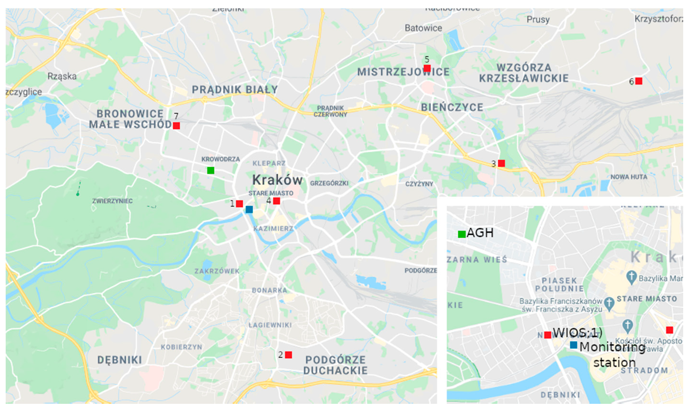
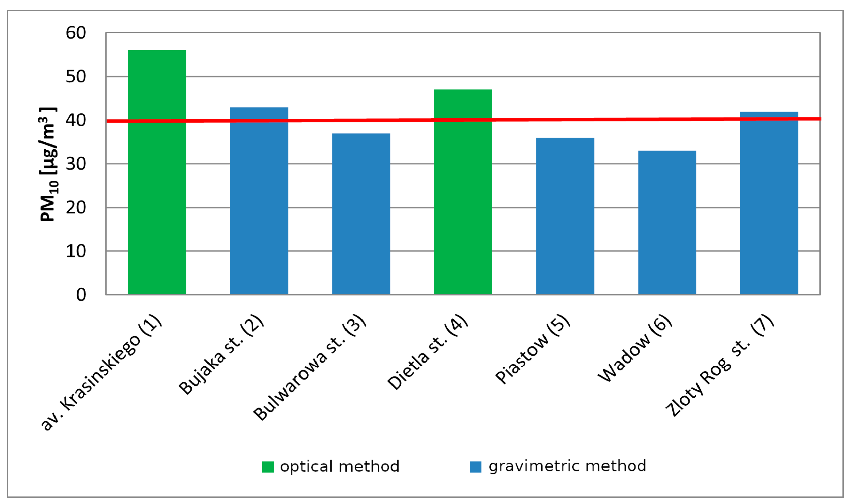
To assess air quality in Krakow for PM
10, measurement series from seven stations (two automatic optical and five manual gravimetrical) were collected and analyzed by the Province Environmental Protection Inspectorate. The locations of all stations are presented in
Figure 1. The most frequently exceeded norm was observed at Krasinski Avenue [
30], and the highest yearly PM
10 number is also observed there (
Figure 2).
To assess air quality in terms of PM
2.5 particulate matter, measurement series from three stations (two automatic and one manual) were analyzed. The average annual concentrations ranged from 39 µg/m
3 at Krasinski Avenue up to 27 µg/m
3 at Bulwarowa Street in 2017 [
30].
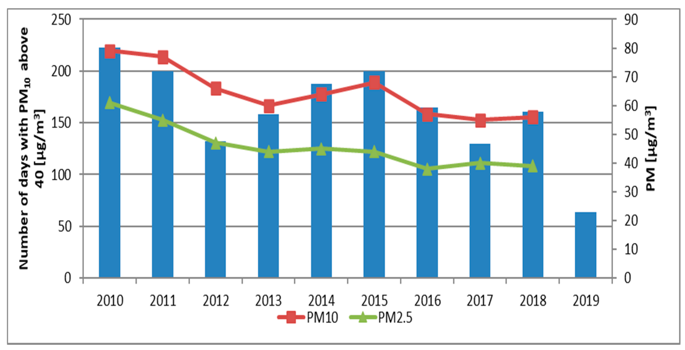
The analysis of the number of exceedances of PM
10 levels showed that the worst year in terms of air quality was 2010, which had 223 exceedances. The data show a decreasing trend, with a period of increased values in 2014–2015 (
Figure 3) and a lower exceedance value in 2012. The concentrations of PM
10 and PM
2.5 show a clear decreasing trend (
Figure 3), but a slight increase in concentrations was visible in the years 2014–2015.
4. Proposed Method
For this project dataset of images, numerical datasets of weather data and air pollution with PM
10 and PM
2.5 data have been used. Proposed method for estimating PM
10 and PM
2.5 in atmospheric air and exceedances of air quality was based on the Cross-Industry Standard Process for Data Mining (CRISP-dm) methodology.
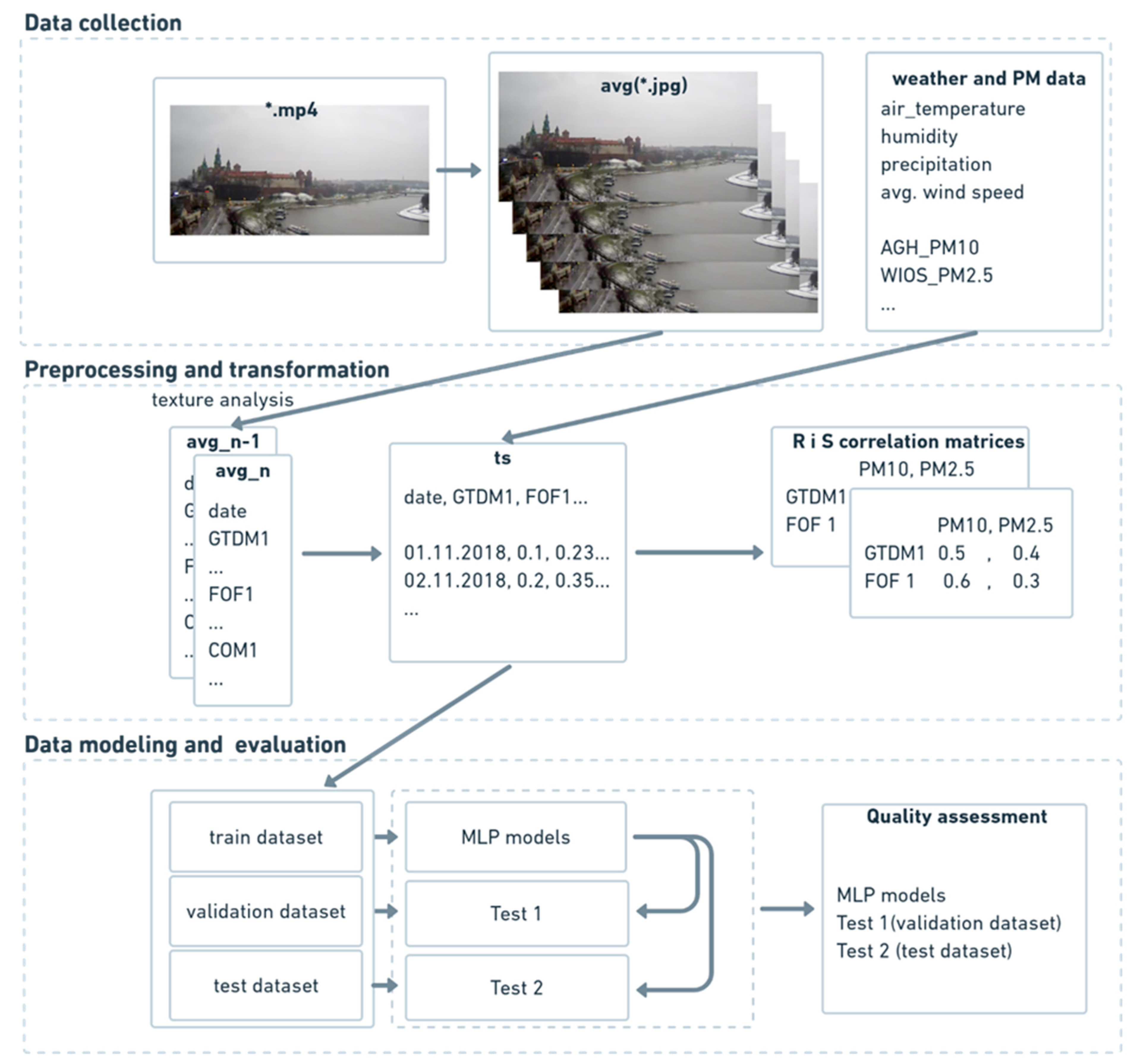
Figure 4 illustrates the block diagram of the proposed method. The authors described the phases presented in
Figure 4 in the following parts of this paper. The proposed method is a transitive method between the use of neural networks to predict air quality based on photos presented in publications [
13,
14,
15] and the approach based on modeling numerical data presented by the authors in [
16,
23,
24]. In the first step, texture analysis for each of the average photo frames has been performed, using three complementary methods. Thanks to the selected methods, a single value for each texture feature was obtained. The next step was to combine the results from the texture analysis, weather, and air pollution data. Then, regression and classification MLP neural networks were performed for numerical data. The selected method allowed for the creation and preliminary evaluation of a single neural network in less than 1 s. In the last step, the quality of selected neural network models was assessed.
4.1. Data Collection
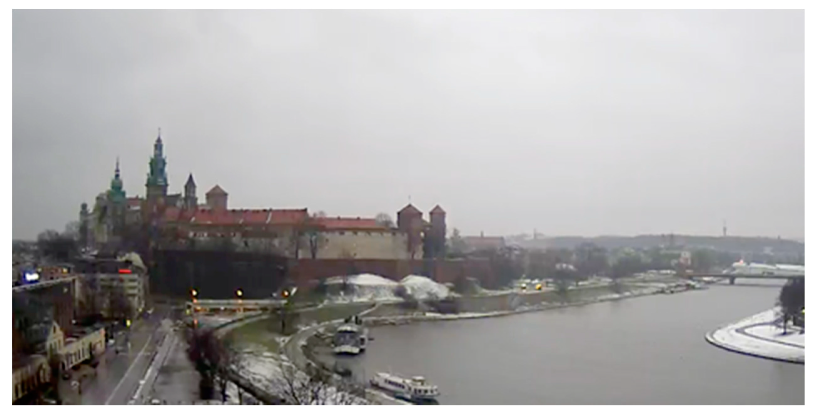
Data analysis was performed on good-quality image data that were acquired daily. Image data acquisition was performed periodically for 100 days (from 21 November 2018 to 28 February 2019) at sunrise (between 7 and 7.30 AM, UTC+1) from the “Wawel castle and the Vistula bend” city monitoring station, whose coordinates are 50°03′ N 19°55′ [
41]. The automated process was downloading videos from the camera according to the aforementioned schedule. Short *.mp4 files (movies with resolution 1920 × 1080 px) were saved in the disk space, from which five random frames were extracted and averaged. Each frame contains the same view presented in
Figure 5. Images carry unstructured sets of pixels; however, each image has a texture that has been analyzed in further steps. On the other hand, weather parameters collected by sensors have been provided as structured *.csv files. The combination of both sources done by the automated process gave the results presented below. To ensure the best possible convergence of parameters, weather and air quality data were collected from two weather stations located in the neighborhood of the image acquisition location, which is presented in
Figure 1.
Weather data were obtained from the weather station run by the Environmental Physics Group of AGH University of Science and Technology in Krakow (AGH), which is shown on the map (
Figure 1) as a green square [
42]. The averaged results of parameter measurements from a full hour were registered. For this period (21 November 2018 to 28 February 2019), 7:00 a.m. was established as a measuring point. The location of the station is 50°04′ N 19°55′ E, and its foundation height is 220 m a.s.l. The weather station provided meteorological information, including average air temperature, average relative humidity, average atmospheric pressure, average wind speed, maximum speed of wind gusts, precipitation and air quality status assessed using the PM
10 indicator. Weather and airborne particulate matter measurements were provided by a Vaisala WXT520 automatic weather station and a Plantower PMS5003 [
42].
Additional air quality status information was obtained from the station of the Voivodeship Inspectorate of Environmental Protection in Krakow (WIOS), located at Krasinski Avenue (
Figure 1) [
43]. The measuring point coordinates are 50°03′ N 19°55′ E; its foundation height is 207 m a.s.l. The station is located close to the “Wawel Castle and Vistula bend” monitoring point, which provided images from webcams. The measuring station at Krasinski Avenue recorded the following parameters: nitrogen oxide content, carbon monoxide content, nitrogen dioxide content, benzene content, PM
10, and PM
2.5 indicators.
4.2. Preprocessing
Every object has a texture that can be used to characterize it. Even if one considers an object to have no texture, image processing methods consider it to have a plain texture. An example of a plain texture is a photograph of a clear sky on a sunny day. When clouds are visible, each of them may have a different texture. Changes in air pollution are also noticeable in photographs and can be reflected as changes in texture. The project used three complementary texture methods presented in
Section 3 on average images from the camera. The textures features were saved into structured *.csv file. In the next step, files with weather data, texture features, and PM data were combined into one file with a time index (see
Figure 4). Such a prepared file was used in correlation analysis and modeling.
4.3. Modeling and Evaluation
Regression and classification of the neural network models were used to assess the possibility of predicting the content of PM10 and PM2.5 in atmospheric air. Moreover, based on image texture parameters and basic meteorological data (air temperature, average wind speed, humidity, precipitation), they were also used to predict the exceedances of air quality standards.
The analyzed particulate matter data from each of the measuring stations were divided into 3 subsets. Since the analyzed data are a time series, the data were not randomly divided into subsets. The oldest 70% of the observations were assigned to the training set, another 15% was assigned to the validation set, and the newest observations were assigned to the test set. One thousand different regression neural networks with different architectures were made for each parameter. The neural network was created using a training dataset with the automatic Data Mining toolbox in Statistica 13.1. The created neural networks had a three-layer structure with one hidden layer. In the hidden layer, we tested from 5 to 25 neurons. The maximum number of epochs was 200, and the stop criterion was 0.00001. The initial weights were random using normally distributed values within a range whose mean is zero and standard deviation is equal to one. These networks differed also in the activation functions of neurons in the hidden layer and the output layer. Each neural network was created based on a training dataset. Successively, the fitted model is used to predict the responses for the observations in a second dataset called the validation dataset. The validation dataset provides an unbiased evaluation of a model fit on the training dataset. In the last step, an unbiased evaluation of a final model fit on the training dataset is performed with the test dataset.
Of all the created networks, the one with the highest quality values for all three datasets and the lowest number of neurons in the hidden layer was selected for each predicted PM dataset, to present in this paper.
Classification methods are sensitive to the unevenness of the occurrence of classes in subsets. Therefore, for the classification methods, only a random selection of observations for individual sets was used to better balance the observations belonging to individual classes. For the classification models, the quantitative data were changed to 3 PM
10 classes. The good air quality class was defined as PM
10 lower than 50 µg/m
3; the poor air quality class was PM
10 between 50 and 100 µg/m
3; and the very poor-quality class was PM
10 higher than 100 µg/m
3. This division was made based on the ordinance of the Polish Minister of the Environment [
28,
29]. For suspended particle matter with a diameter smaller than 2.5 micrometers, two classes were distinguished: air quality is considered good if dust content is lower than 25 µg/m
3, and it is considered poor for higher values [
28]. The same as for the regression models, one thousand models were created automatically for each PM dataset, with the same conditions as presented in previous paragraph; from these, only the ones with the highest quality were used in the tests.
4.4. Software
The project was implemented on computers with a Windows 10 × 64-bit system with an Intel Core i7-3630QM CPU 2.4 GHz processor, 16 GB RAM, and a Windows 10 × 64-bit system with an Intel Core i7-10710U CPU 1.10 GHz processor, 16 GHz RAM. In this project, we used specialized software, computing platforms, and programming languages for statistical computing and graphics. For texture analysis, we used MATLAB 2016a, which is a programming and numeric computing platform. Correlation matrices and quality assessment were prepared in the R × 64 4.0.2 language with function cor from stats package version 3.6.2, and caret package version 6.0–88. Neural networks were created in the Statistica 13.1 64-bit program with SANN toolbox for automatic neural network building.
5. Results
Data analysis was performed to assess the relationship between dust suspended in atmospheric air and the texture parameters calculated from the averaged film frames recorded at sunrise and the basic weather data: air temperature, humidity, precipitation, average wind speed. The following analyses were carried out in sequence: Pearson’s linear correlation, Spearman’s rank nonlinear correlation, MLP regression neural network model, and MLP neural network classification models.
In the first step, the relationship between the measurement stations for the recorded suspended PM
10 dust measurements was determined. The linear correlation coefficient between PM
10 at AGH station and PM
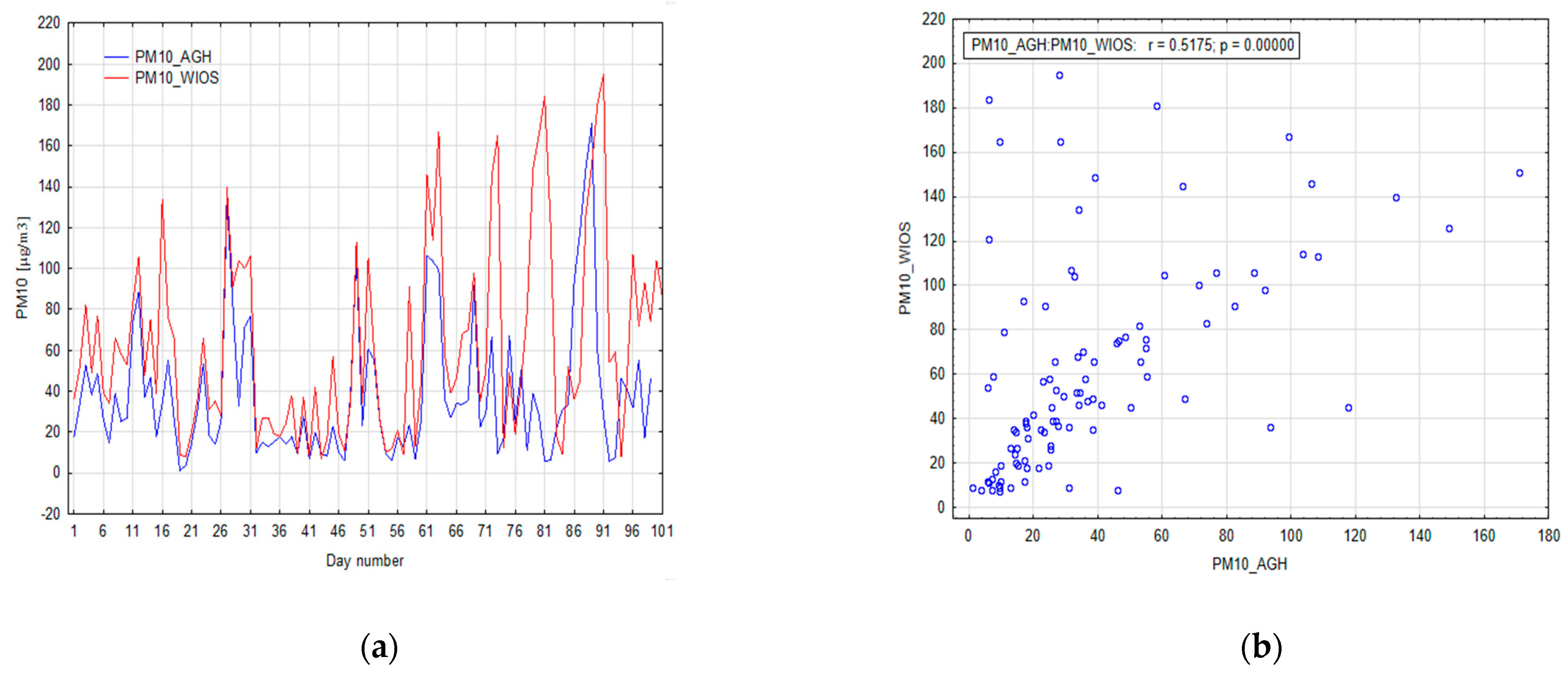
10 at WIOS is 0.52. The value of the Spearman’s rank correlation is slightly higher, which indicates the presence of nonlinear relationships between these stations (0.6). This is a relatively low similarity when it is considered that the stations are only about one kilometer apart. The analysis of the line graph of both PM
10 datasets shows that the data are positively correlated with each other (
Figure 6a), but there are also significant differences in mean values and variation between those two stations (
Figure 6a). Differences between measurements are smaller for low PM
10 values (
Figure 6b). As the measured values increase, the difference between the PM
10 datasets also increases. In
Figure 6a, two periods are visible with very high differences between the PM
10 WIOS station and PM
10 AGH station values. The first period is 70–73 observations with a maximum of 73 observations. The difference between measurements is 155.6 µg/m
3. The second period is 76–81 observations with a maximum of 81 observations. The difference between measurements is 178 µg/m
3. Both days with very high differences in measurements are days with negative air temperature lower than −5 °C, with an average wind speed lower than 1.5 m/s and without precipitation. Both periods are in a validation dataset. This may be related to the fact that the WIOS station is located in a green area in the middle of a busy road, while the AGH station is located near a less busy road on the AGH campus.
Based on the correlation analysis, we can conclude that there is a significant variation in PM content even over short distances; therefore, the models will be local in nature and will only be accurate in the immediate vicinity. In the next step, the relationship between the measurements for the WIOS station was computed. The Pearson’s correlation coefficient between PM2.5 and PM10 is 0.89. The value of the Spearman’s rank correlation is slightly lower, which indicates the presence of strong linear relationships between these stations (0.87).
The correlations between PM
10, PM
2.5, and texture parameters as well as air temperature, precipitation, and air humidity were calculated. Pearson’s linear correlation coefficient was used to assess linear relationships; Spearman’s rank coefficient was used to assess nonlinear relationships. In the Pearson’s correlation coefficients, the results with the highest correlation coefficient values for texture parameters (
Table 2) were obtained using the GTDM method. All texture parameters are statistically significant with the PM
10 and PM
2.5 datasets. The highest correlation coefficient values were observed for PM
10 from the WIOS station. In the FOF method, only two parameters correlated at a significant level for PM
10 from the WIOS station (FOF1, FOF3). PM
10 from the AGH station and PM
2.5 were not significantly correlated with First-order Feature texture data. In Haralick’s method, almost all texture parameters correlated with PM
10 WIOS; only correlations with COM1, COM8, and COM14 were not statistically significant (
p > 0.05). Pearson’s correlation coefficients obtained for PM
2.5 at WIOS and PM
10 at AGH were weaker: 4% and 10%, respectively. Furthermore, the number of statistically significant correlations decreased: 20 for PM
10 WIOS, 15 for PM
2.5 WIOS, and 12 for PM
10 AGH (
Table 2). The highest Pearson’s correlation coefficient value was observed for the correlation between average wind speed and PM
10 at WIOS station (−0.626). Moreover, Pearson’s correlation coefficient between PM
2.5 from WIOS station and the average wind speed equals −0.58. It is visible that a medium-strength negative relationship exists between PM data and average wind speed. The highest correlation between PM datasets and texture parameters was observed between PM
2.5 from WIOS station and GTDM2 (−0.485).
When comparing the results of the two correlation methods, the Spearman correlation coefficient was found to have higher values. The number of statistically significant correlations increases for PM10 from the AGH station. For all stations, the FOF4 and COM1 Spearman rank correlation coefficients are higher than Pearson’s correlation coefficients and are statistically significant.
For PM10 AGH, four more statistically significant correlations were measured with Spearman rank correlation than with the Pearson correlation coefficient: FOF4, COM1, COM3, and COM13. The highest changes in correlation values between the Pearson and Spearman correlation coefficients are visible for Haralick’s texture parameters: 0.241 (correlation was measured between COM10 and PM10 WIOS). When comparing the results of the two correlation methods, higher values for Spearman’s correlation coefficient are visible. The number of statistically significant correlations increases especially for PM10 from AGH station. For all stations, the FOF4 and COM1 correlation values increased and became statistically significant compared to the Pearson correlation coefficient. For PM10 from AGH station, four more statistically significant correlations were measured with Spearman rank coefficient (FOF4, COM1, COM3, COM13).
Due to the nonlinear relationships between PM data and texture parameters, a multilayer perceptron was used as a regression model. Texture parameters and weather data were chosen as independent variables, and they showed a statistically significant correlation with PM data. The number of neurons in the input layer equals the number of variables in the model. The variables used in the models are marked in dark blue italics in
Table 2. From the 1000 neural networks that were created for each PM dataset, only the one with highest quality was chosen for tests.
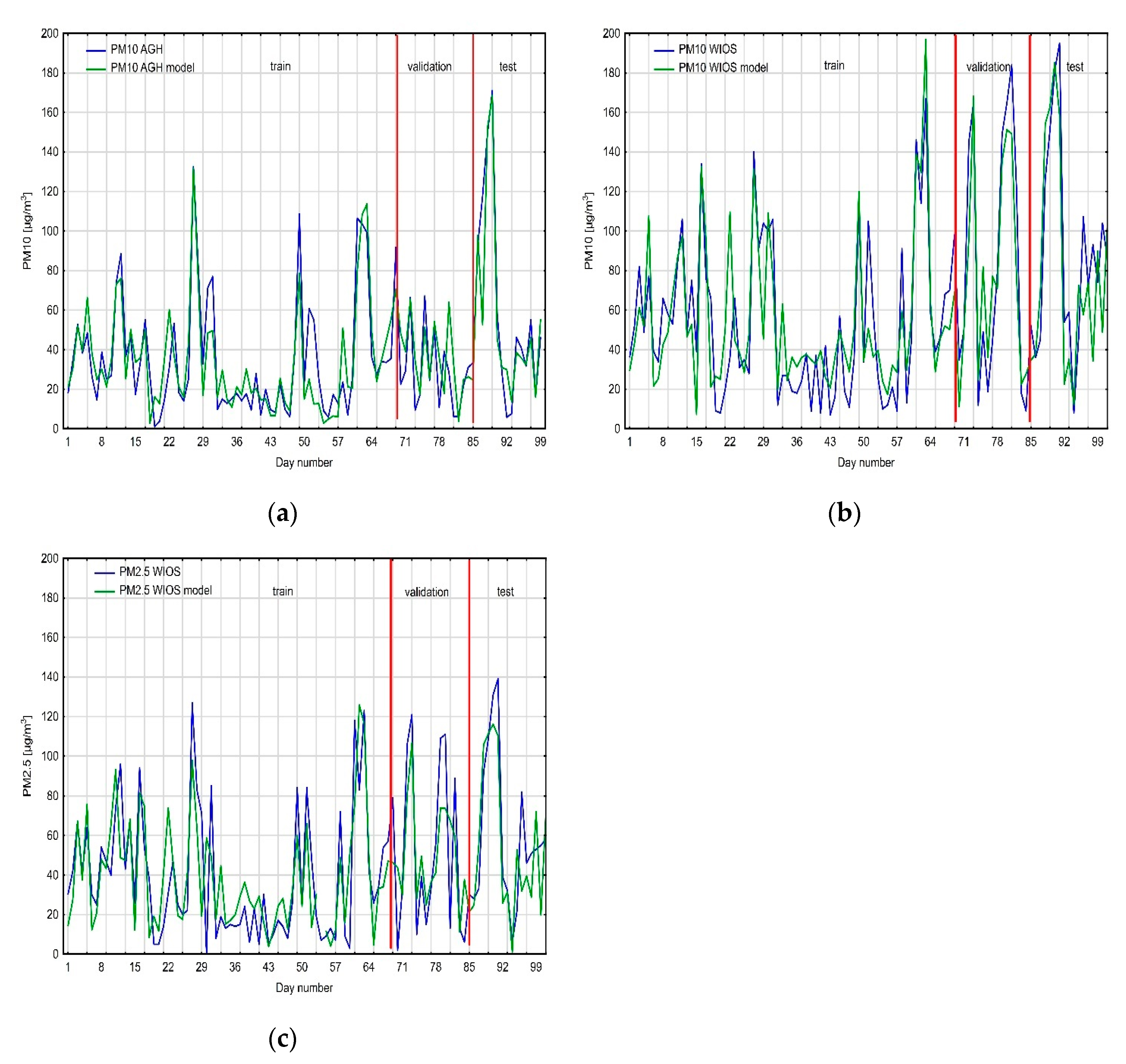
The regression neural network prediction for PM10 values from the AGH measuring station consisted of 17 neurons in the input layer. The best network presented in the results had one hidden layer consisting of seven neurons, and an output layer with one neuron. An exponential function was chosen as the hidden layer activation function, and the neuron activation function in the output layer was linear. Learning, validation and testing qualities are high: 0.9, 0.8, and 0.85, respectively. The neural network algorithm required 57 epochs. The neural network that predicted PM10 values from WIOS station had two more neurons in the input layer and two fewer neurons in the hidden layer. The activation functions are the same as for the first neural network. Learning quality is similar to the first neural network (0.89); validation quality is higher (0.9); however, testing quality is lower (0.73). This neural network required 34 epochs. The last neural network, which predicted PM2.5 values, had 14 neurons in the input and hidden layers, and one neuron in the output layer. Its activation functions differ from the previous networks: in the hidden layer, we used the logistic function; in the output layer, we used the hyperbolic tangent; the learning process takes 26 epochs. The learning, validation, and testing qualities are the lowest from all the three neural networks: 0.8, 0.84, and 0.63, respectively. The coefficient of determination (R2) was computed for learning, validation, and test datasets. For PM10, AGH equals 0.81, 0.64, and 0.72, respectively. The R2 for PM10 WIOS are 0.79, 0.81, and 0.53. Lower R2 values were computed for PM2.5 WIOS: 0.64, 0.70, and 0.40.
Moreover, the models’ qualities were checked with mean error (ME) in the test dataset and mean absolute percentage error (MAPE). The MAPE values for the test dataset equal 27% (PM
10 AGH), 13% (PM
10 WIOS), and 19% (PM
2.5 WIOS). The MEs for the test datasets equal 3.7, 5.5, and 3.9, respectively. The high ex-post measure values for the created models relate to differences in the dataset. The test datasets had higher variability than the training datasets for all PM data (
Figure 7).
Air quality assessment of PM10 and PM2.5 exceedances was performed based on the MLP network. According to the ordinance of the Minister of the Environment, the PM data were divided into three classes (PM10) and two classes (PM2.5). The number of classes determined the number of neurons in the created networks’ output layers.
The best three neural networks were tested. The architecture differences between these neural networks are significant. The PM
10 AGH neural network has 17 neurons in the input layer and nine neurons in the hidden layer. All statistically significantly correlated variables were used in the model (
Table 2). The activating functions of the neurons were hyperbolic tangent and softmax. A more extensive network was obtained for PM
10 WIOS, in which the input layer had one more neuron and the same number of neurons in the hidden layer as PM
10 AGH. This network is additionally distinguished by the functions of the activating neurons in the hidden and output layers: logistics and hyperbolic tangent, respectively. The last PM
2.5 WIOS neural network had 17 neurons in the input layer and 12 neurons in the hidden layer, and the activation functions were hyperbolic tangent and softmax, respectively.
The obtained percentage of correct classifications (accuracy * 100%) in the learning datasets varies from 87.3% for PM10 AGH to 94.4% for PM2.5 WIOS. For PM10 WIOS, the percentage of correct classification is 92%. The percentage of misclassifications is evenly distributed over the classes. The percentage of correct classifications in the validation datasets are 92% for PM10 AGH, 71% for PM10 WIOS, and 85% for PM2.5 WIOS. The quality of the neural networks in the test dataset is lower than in the learning dataset, but it is still high, and in the worst case (PM2.5 WIOS), it achieves 80% of correct classifications. The best results were obtained by the network that predicts PM10 AGH class. The test set achieved 92.9% correct classifications. PM10 WIOS obtained 85.7% correct classifications in the test dataset. The Area under Curve (AUC) values computed for whole datasets are 0.792 for PM10 AGH, 0.802 for PM10 WIOS, and 0.928 for PM2.5 WIOS.
The created confusion matrix for the test dataset shows that no error repeats constantly (
Table 3). All the neural networks have one wrong classification, where poor air quality was classified as good. Two observations classified as “good” were classified as poor in PM
2.5 WIOS, thus giving a total of only 80% of correct classifications. In addition, for PM
10 WIOS, one additional wrong classification was observed: poor air quality was classified as very poor (
Table 3).
6. Conclusions, Limitations, and Future Research
The issue of air pollution, including the particulate matter, has been extensively presented in the literature [
1,
2,
3,
24]. This is a key issue for most urbanized areas, especially for big agglomerations [
4,
14,
16,
23,
24,
44]. Air pollution in Poland is a big problem, especially in urbanized areas [
22]. In the analyzed period in the city of Krakow, exceedances of the permissible standards presented in
Table 1 were observed over 100 times a year (
Figure 3). Due to frequency with which air quality limits were exceeded, cheap and effective tools are needed to quantify and qualify air quality.
The assessment of PM air pollution is commonly carried out using various types of methods discussed in the literature [
5,
6,
7,
8,
9]. Carretero-Peña et al. (2019) and Sarimveis et al. (2006) proposed assessing air quality using image analysis. The assessment of air pollution with particulate matter is often based on images and images analysis. Papers presented models based on images analysis with Gabor filter [
13], conversion to gray scale, and the Otsu method [
18]. Liu et al. also proposed using six image features: transmission, whole image and local image contrast, entropy, sky smoothness, and color. The authors in [
25] used Dark Channel Prior for transmission matrix estimation from multiple scene images. In paper [
45], the authors used the Gray-level Co-occurrence Matrix method (COM) for texture feature extraction in PM assessment. In this paper, we used COM and two additional complementary textures methods: FOF and GTDM. Additionally, in previous research [
20], RBF neural networks were used for the quantitative estimation of air quality, which was assessed with quality measures of ex-post forecast assessment. This paper also proposes the use of artificial neural networks; however, in the work of Ordieres et al., the MLP multilayer perceptron proved to be a better solution [
17]. The use of MLP neural networks to predict air pollution on the basis of numerical data was presented by the authors in [
16,
17]. In paper [
16], the authors use numerical variables and a K-mean algorithm for PM
10 prediction with MLP and MLR. The R was between 0.67 and 0.77, depending on measurement localization for the regression model. Better regression results were obtained with CNN models with the PMIE method: R
2 was between 0.68 (multiple-scene images) and 0.91 (single-scene images) for PM
2.5 prediction [
15]. The main limitation in using CNN is a small dataset of images. In paper [
13], the authors presented shallow (Random Forest) and deep classifiers (CNN) for five-class air quality assessment for an Air Quality Index (AQI). The authors used a method for multiple-scene images and obtained an AUC of 0.6 and an accuracy of 0.53. A very similar approach to modeling was used in this article by adding texture features as additional variables. Additionally, a similar application of texture analysis in PM
2.5 prediction was presented in [
18] for images from China and United States. The main difference between [
18] and this paper is in the used methods: six texture features versus three texture methods. Quality SVR models for Beijing were between 0.68 and 0.7 R
2, for Shanghai, between 0.72 and 0.76 R
2. The air quality analysis was based on analysis of textures on averaged images with full HD resolution: 1920 × 1080 px. The texture features were measured using three methods: The First-order Features, the Neighborhoods Gray-tone Difference Matrix method, and the Gray-Level Co-occurrence Matrix. For each of the three methods, statistically significant nonlinear correlations were demonstrated between the texture parameters and PM
10 AGH, PM
10 WIOS, and PM
2.5 WIOS data. The correlations are weak to moderate. The highest correlation value is −0.518 between COM2 and PM
10 WIOS. Based on the results obtained from the correlation analysis, two types of neural networks were created: regression and classification. Both types of networks had a satisfactory quality. The regression models obtained quality (R) in the 0.63–0.85 range for the test sets. However, the R
2 vary from only 0.4 for PM
10 AGH in the test dataset to 0.81 for PM
10 AGH in the learning dataset, and PM
10 WIOS in the validation dataset. Relatively low R
2 values for PM
10 AGH show model weakness, especially in validation and test datasets. What is more, the calculated MAPE value exceeds 10% for all the regression networks, which indicates that they will probably not be good enough to use, despite the relatively low average errors of these networks: PM
10 AGH—3.7; PM
10 WIOS—5.5; PM
2.5 WIOS—3.9. The datasets used in the tests have high variation and higher mean values than in the learning datasets, so the neural network algorithms did not correctly predict data variation. This could be changed by using longer time series in each dataset. Better results were obtained with the classification models than with the regression models. The worst quality was obtained for the PM
2.5 WIOS classification in the test dataset: 80% (
Table 3). The qualities of other neural networks are equal and higher than 85%. The higher the AUC, the better the performance of the model at distinguishing between classes. The lowest AUC was calculated for PM
10 AGH (0.792). The highest AUC equals 0.928 and was calculated for PM
2.5 WIOS. High AUC values indicate a good fit of the classification models to the data.
The results of this study indicate that photo texture analysis could be useful in air quality assessment. All chosen texture methods were useful in the performed analysis. Additionally, it is possible to predict air quality exceedances by analyzing textures in HD photos with basic weather data as additional information. It is also possible to predict the values of PM10 and PM2.5 in atmospheric air, but these results have a greater error. This error could probably be minimized by using a longer period of data in the learning dataset that contains all seasons, or higher resolution photos, e.g., 4 K.
The obtained models could be used as part of an application for air quality control using smartphone camera photographs, especially for checking air quality because of the high quality and sensitivity of the PM
10 model (higher than 90%). Currently, image sensors are widely accessible, for example, in online cameras and smartphones [
21]. Existing infrastructure could be used to provide more photos to create better air quality models. Classification models could be even implemented in mobile phone applications, which will make analysis more accessible for end users. Future work should focus on building a process that will continuously examine images captured at different locations. Such a constant stream of input data combined with weather data will give a much better model that will assess air quality over a larger area. The limitation of this approach is not only the quality of the camera sensor but also the registered image itself. Night-time photos are not providing enough information for the model; the same applies to photos taken in bad weather conditions. Both of these aspects can be eliminated with the use of appropriate lighting and background, but at the same time, it would make this method much more difficult and more expensive to implement.


