
A Factor-Graph-Based Approach to Vehicle Sideslip Angle Estimation


Abstract
:1. Introduction
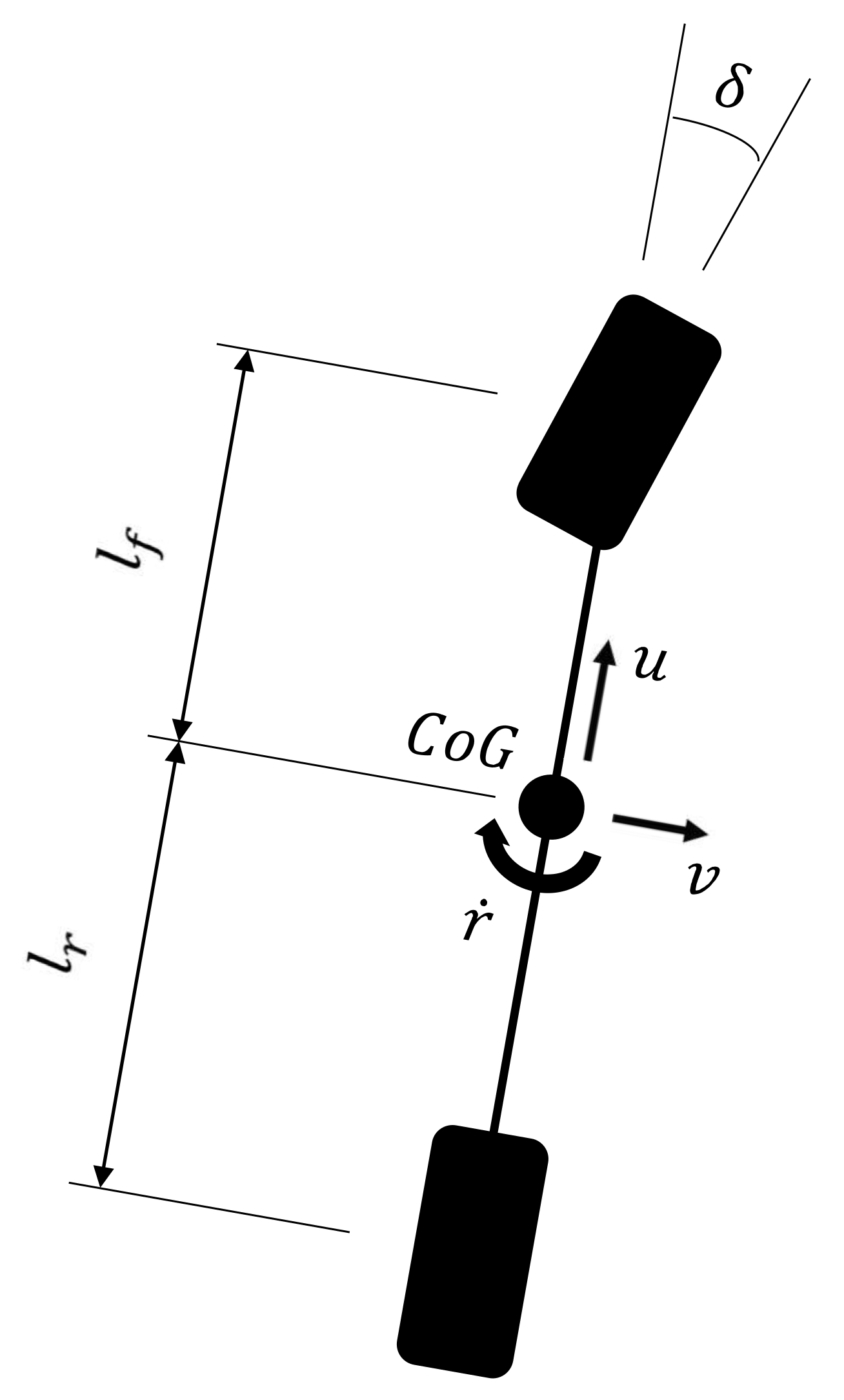
2. Vehicle Dynamic Model
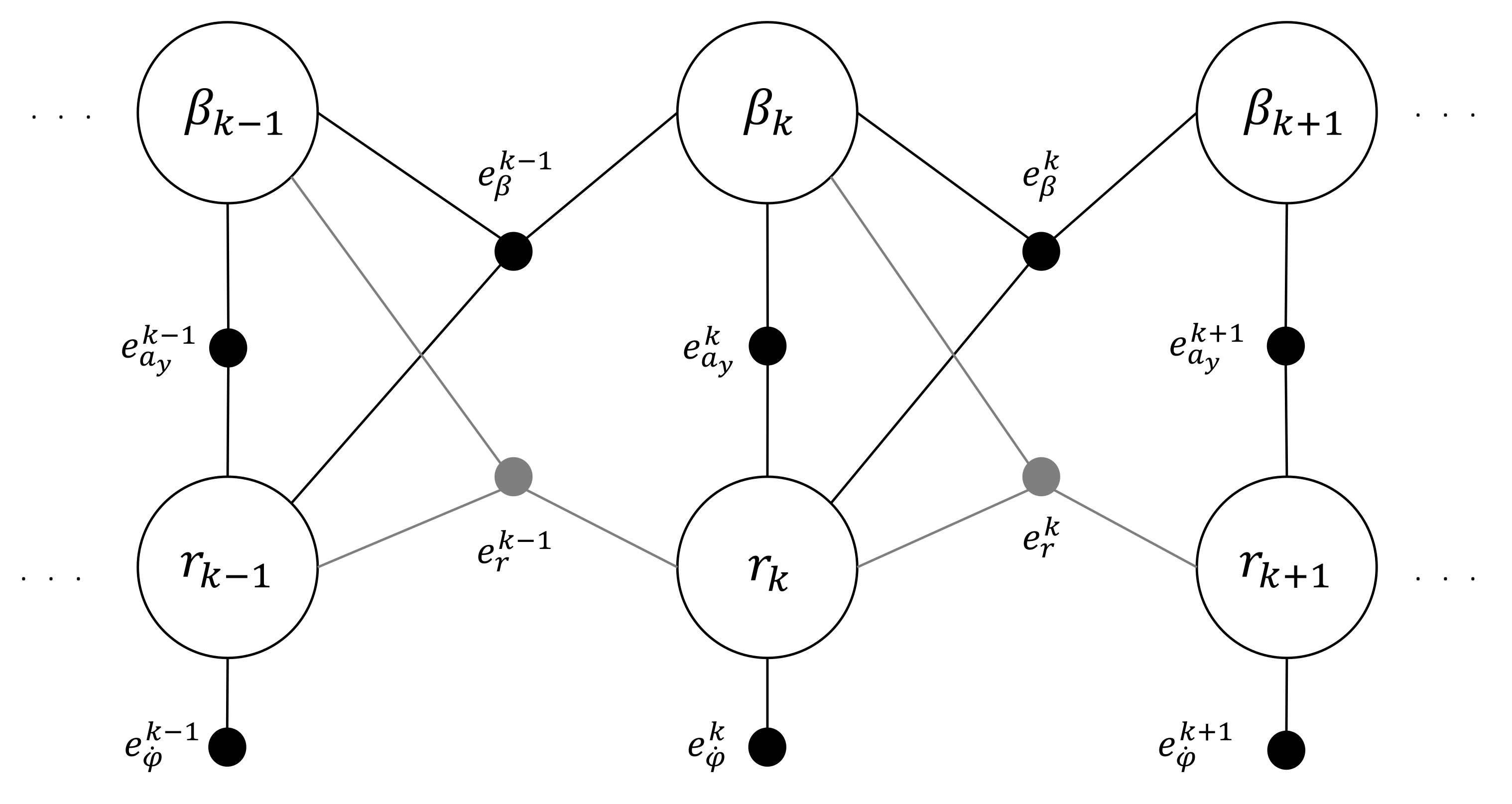
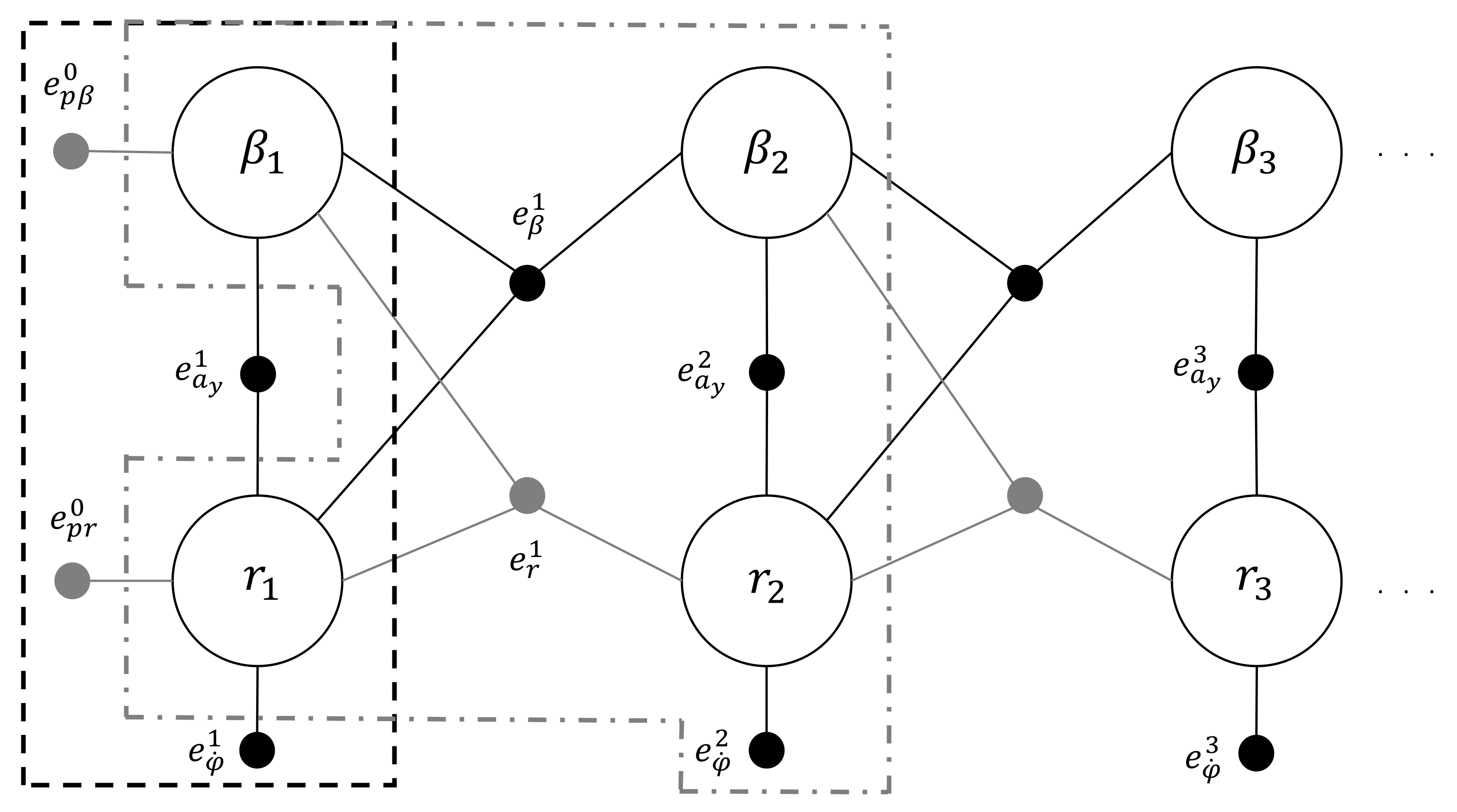
3. Factor Graph for Vehicle Lateral Dynamics
3.1. The Estimation Problem
3.2. Implementation
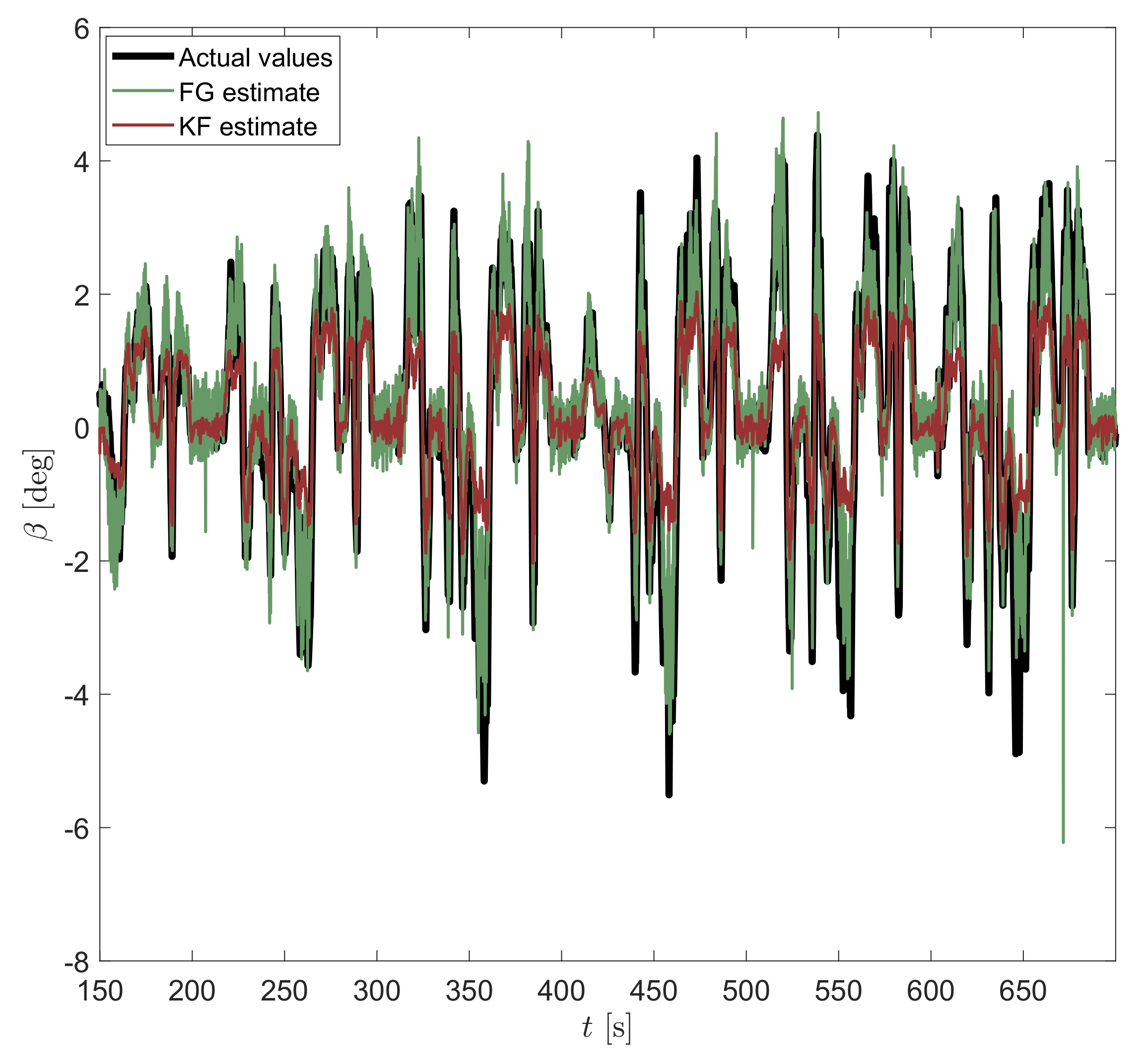
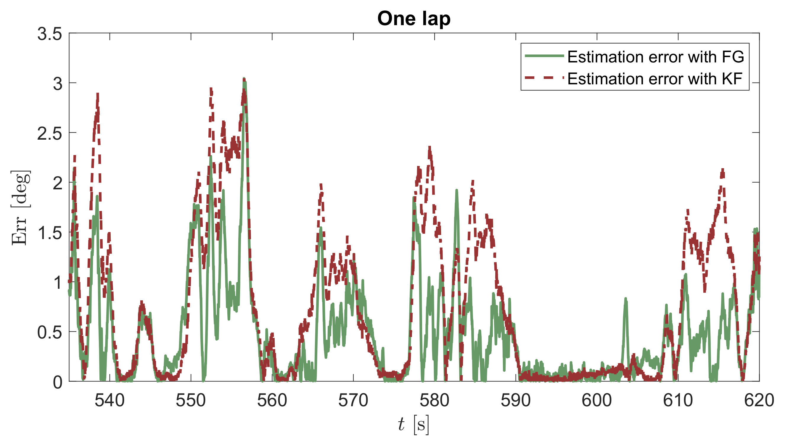
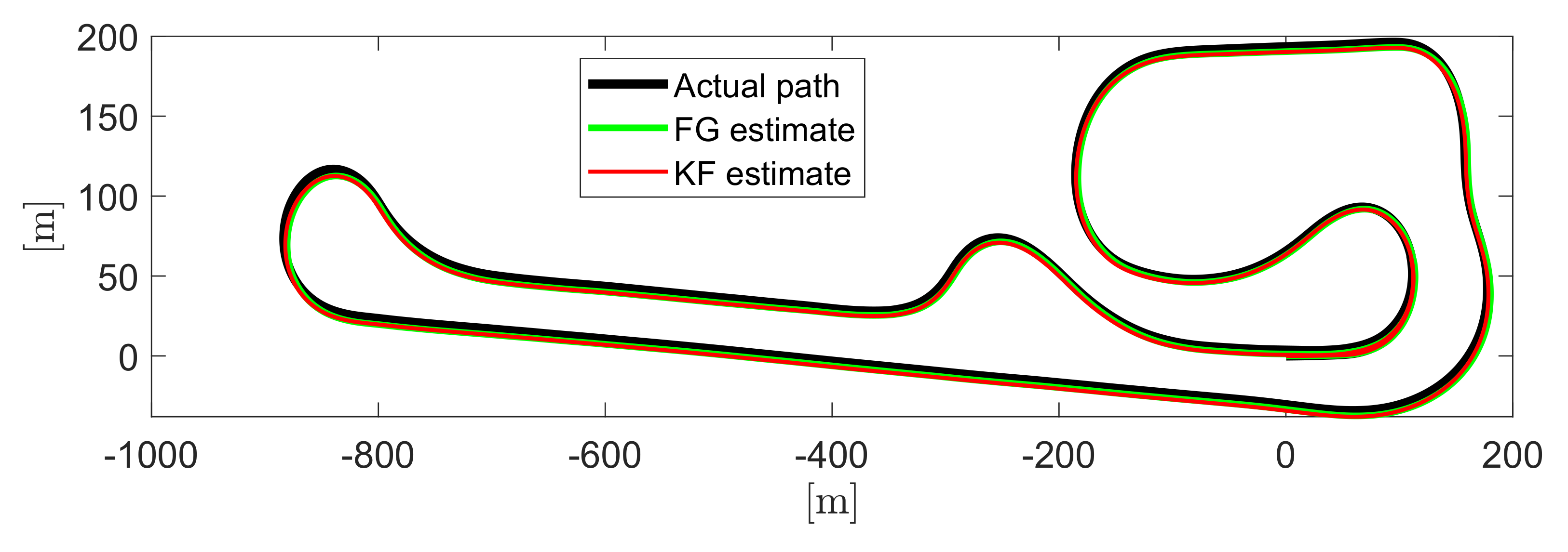
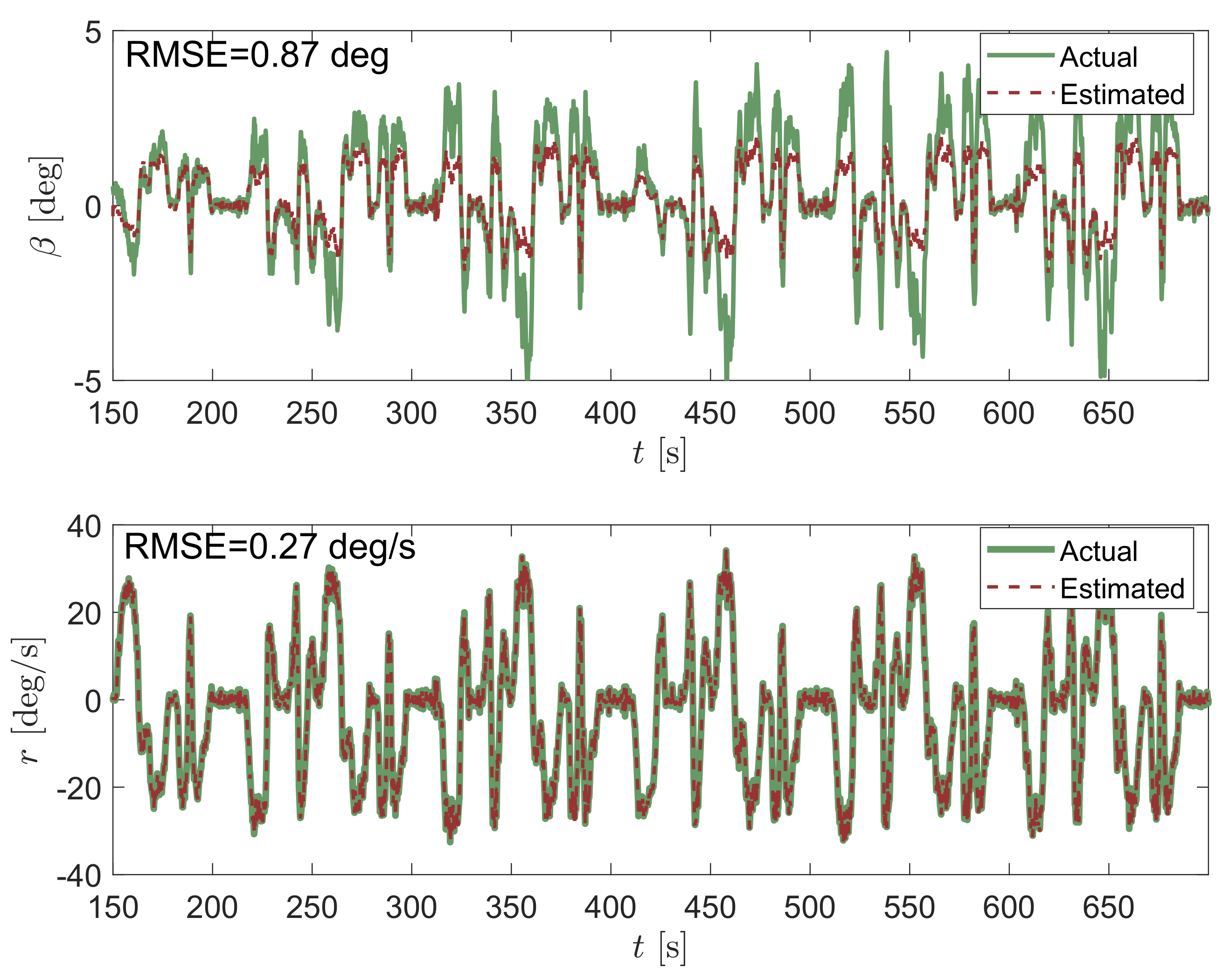
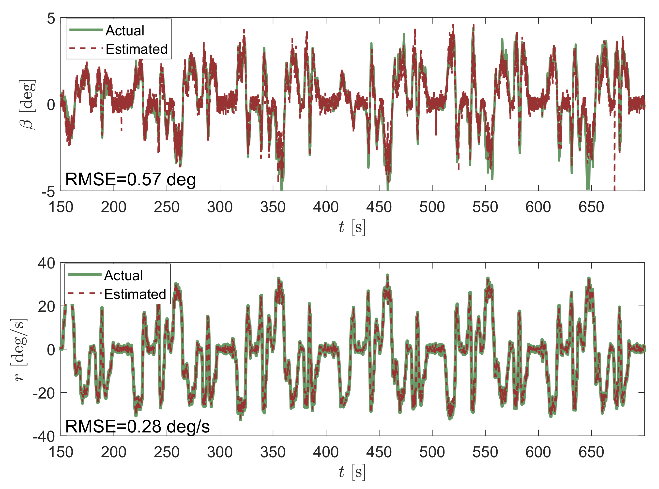
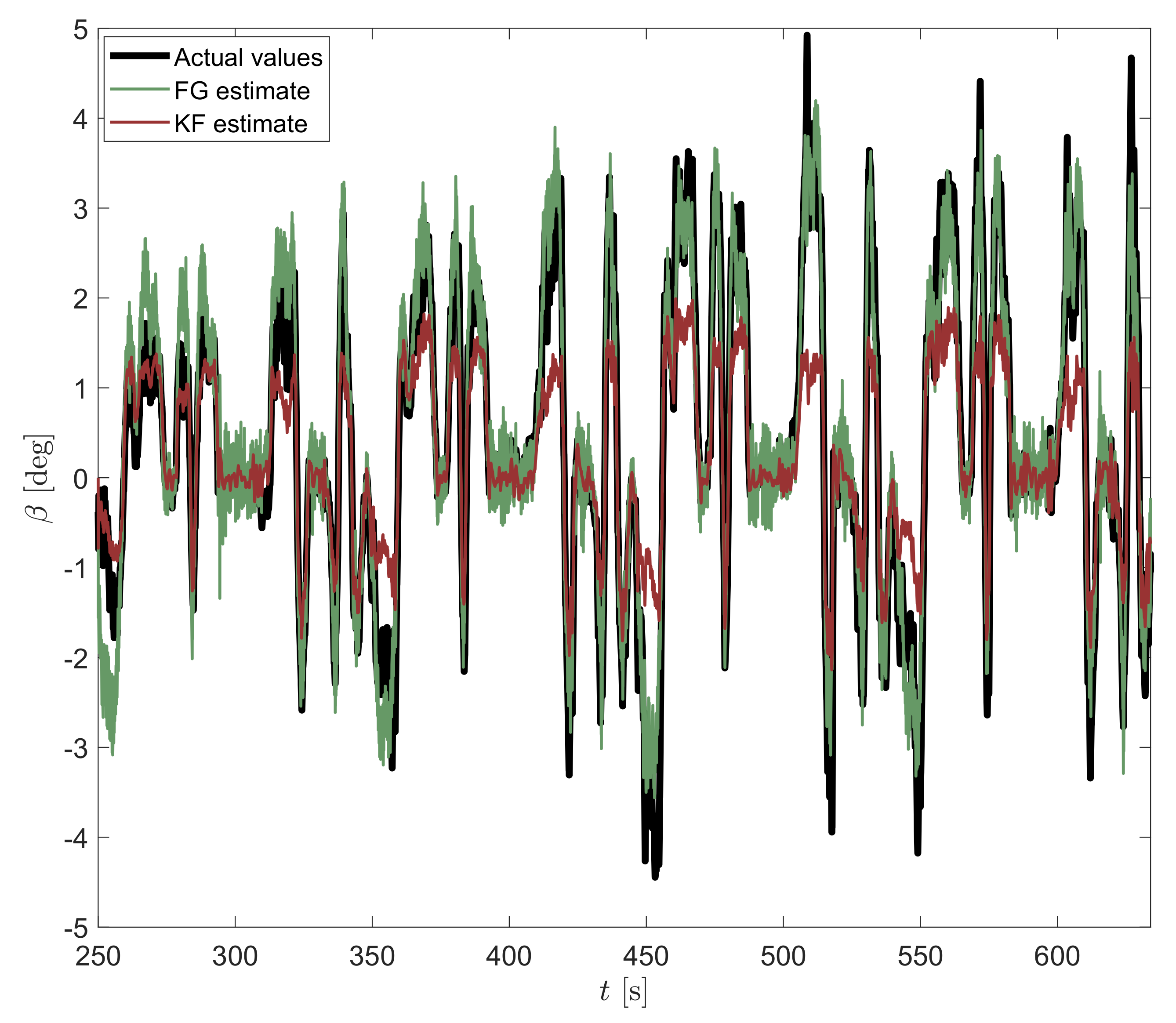
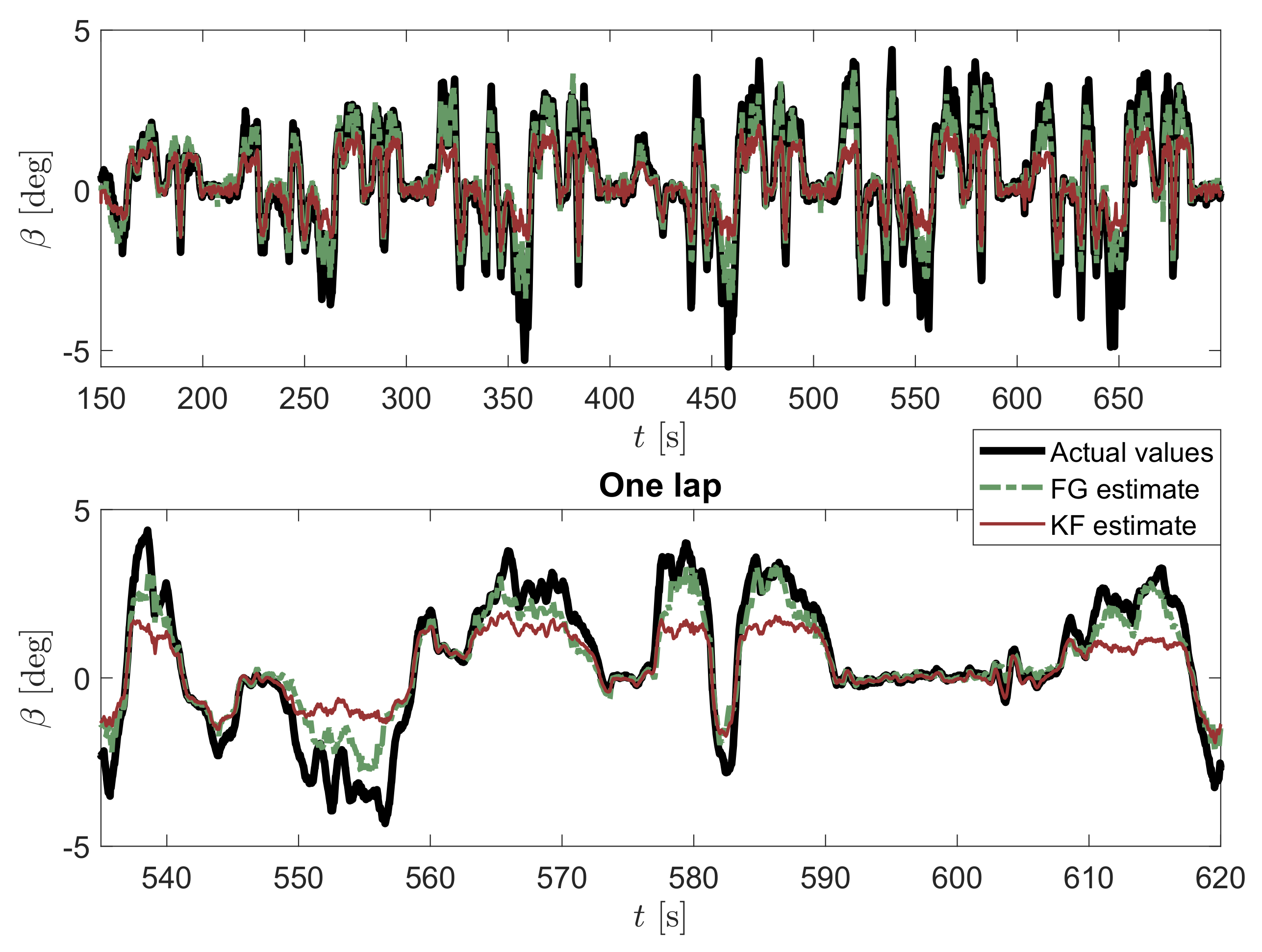
4. Results
5. Conclusions
Author Contributions
Funding
Institutional Review Board Statement
Informed Consent Statement
Conflicts of Interest
Appendix A
- For priors, the actual value is the guess and the function is the difference between these two values; hence:and follows the same rationale.
- For dynamic factors, the actual value is zero, since it is the difference between the forward value and the same obtained by integrating the differential equation; for instance:and follows the same rationale.
- Finally, measures follow this rationale (only yaw rate is taken for the sake of brevity):
References
- Chindamo, D.; Lenzo, B.; Gadola, M. On the vehicle sideslip angle estimation: A literature review of methods, models, and innovations. Appl. Sci. 2018, 8, 355. [Google Scholar] [CrossRef] [Green Version]
- Tin Leung, K.; Whidborne, J.F.; Purdy, D.; Dunoyer, A. A review of ground vehicle dynamic state estimations utilising GPS/INS. Veh. Syst. Dyn. 2011, 49, 29–58. [Google Scholar] [CrossRef]
- Caroux, J.; Lamy, C.; Basset, M.; Gissinger, G.L. Sideslip angle measurement, experimental characterization and evaluation of three different principles. IFAC Proc. Vol. 2007, 40, 505–510. [Google Scholar] [CrossRef]
- Manning, W.; Crolla, D. A review of yaw rate and sideslip controllers for passenger vehicles. Trans. Inst. Meas. Control 2007, 29, 117–135. [Google Scholar] [CrossRef]
- Mastinu, G.; Plöchl, M. Road and Off-Road Vehicle System Dynamics Handbook; CRC Press: Boca Raton, FL, USA, 2014. [Google Scholar]
- Lenzo, B.; Sorniotti, A.; Gruber, P.; Sannen, K. On the experimental analysis of single input single output control of yaw rate and sideslip angle. Int. J. Automot. Technol. 2017, 18, 799–811. [Google Scholar] [CrossRef]
- Best, M.C.; Gordon, T.; Dixon, P. An extended adaptive Kalman filter for real-time state estimation of vehicle handling dynamics. Veh. Syst. Dyn. 2000, 34, 57–75. [Google Scholar]
- Cheli, F.; Melzi, S.; Sabbioni, E. An adaptive observer for sideslip angle estimation: Comparison with experimental results. In Proceedings of the ASME 2007 International Design Engineering Technical Conferences and Computers and Information in Engineering Conference, Las Vegas, NV, USA, 4–7 September 2007; Volume 48043, pp. 1193–1199. [Google Scholar]
- Antonov, S.; Fehn, A.; Kugi, A. Unscented Kalman filter for vehicle state estimation. Veh. Syst. Dyn. 2011, 49, 1497–1520. [Google Scholar] [CrossRef]
- Wei, W.; Bei, S.; Zhu, K.; Zhang, L.; Wang, Y. Vehicle state and parameter estimation based on adaptive cubature Kalman filter. ICIC Express Lett. 2016, 10, 1871–1877. [Google Scholar]
- Luo, W.; Wu, G.; Zheng, S. Design of vehicle sideslip angle observer with parameter adaptation based on HSRI tire model. Automot. Eng. 2013, 33, 249–255. [Google Scholar]
- Reina, G.; Paiano, M.; Blanco-Claraco, J.L. Vehicle parameter estimation using a model-based estimator. Mech. Syst. Signal Process. 2017, 87, 227–241. [Google Scholar] [CrossRef] [Green Version]
- Reina, G.; Messina, A. Vehicle dynamics estimation via augmented Extended Kalman Filtering. Measurement 2019, 133, 383–395. [Google Scholar] [CrossRef]
- Xin, X.; Chen, J.; Zou, J. Vehicle state estimation using cubature kalman filter. In Proceedings of the 2014 IEEE 17th International Conference on Computational Science and Engineering, Chengdu, China, 19–21 December 2014; pp. 44–48. [Google Scholar]
- Cheli, F.; Sabbioni, E.; Pesce, M.; Melzi, S. A methodology for vehicle sideslip angle identification: Comparison with experimental data. Veh. Syst. Dyn. 2007, 45, 549–563. [Google Scholar] [CrossRef]
- Di Biase, F.; Lenzo, B.; Timpone, F. Vehicle sideslip angle estimation for a heavy-duty vehicle via Extended Kalman Filter using a Rational tyre model. IEEE Access 2020, 8, 142120–142130. [Google Scholar] [CrossRef]
- Dakhlallah, J.; Glaser, S.; Mammar, S. Vehicle side slip angle estimation with stiffness adaptation. Int. J. Veh. Auton. Syst. 2010, 8, 56–79. [Google Scholar] [CrossRef]
- Chen, Y.; Ji, Y.; Guo, K. A reduced-order nonlinear sliding mode observer for vehicle slip angle and tyre forces. Veh. Syst. Dyn. 2014, 52, 1716–1728. [Google Scholar] [CrossRef]
- Syed, U.H.; Vigliani, A. Vehicle Side Slip and Roll Angle Estimation; Technical Report; SAE Technical Paper; Politecnico di Torino: Turin, Italy, 2016. [Google Scholar]
- Pacejka, H. Tire and Vehicle Dynamics; Elsevier: Amsterdam, The Netherlands, 2005. [Google Scholar]
- Davoodabadi, I.; Ramezani, A.A.; Mahmoodi-k, M.; Ahmadizadeh, P. Identification of tire forces using Dual Unscented Kalman Filter algorithm. Nonlinear Dyn. 2014, 78, 1907–1919. [Google Scholar] [CrossRef]
- Reina, G.; Leanza, A.; Mantriota, G. Model-based observers for vehicle dynamics and tyre force prediction. Veh. Syst. Dyn. 2021, 1–26. [Google Scholar] [CrossRef]
- You, S.H.; Hahn, J.O.; Lee, H. New adaptive approaches to real-time estimation of vehicle sideslip angle. Control. Eng. Pract. 2009, 17, 1367–1379. [Google Scholar] [CrossRef]
- Chindamo, D.; Gadola, M. Estimation of vehicle side-slip angle using an artificial neural network. MATEC Web Conf. 2018, 166, 02001. [Google Scholar] [CrossRef] [Green Version]
- Wei, W.; Shaoyi, B.; Lanchun, Z.; Kai, Z.; Yongzhi, W.; Weixing, H. Vehicle sideslip angle estimation based on general regression neural network. Math. Probl. Eng. 2016, 2016, 3107910. [Google Scholar] [CrossRef] [Green Version]
- Cheli, F.; Ivone, D.; Sabbioni, E. Smart Tyre Induced Benefits in Sideslip Angle and Friction Coefficient Estimation. In Sensors and Instrumentation; Springer: Berlin/Heidelberg, Germany, 2015; Volume 5, pp. 73–83. [Google Scholar]
- Melzi, S.; Resta, F.; Sabbioni, E. Vehicle Sideslip Angle Estimation Through Neural Networks: Application to Numerical Data. Eng. Syst. Des. Anal. 2006, 42495, 167–172. [Google Scholar]
- Koller, D.; Friedman, N. Probabilistic Graphical Models: Principles and Techniques; MIT Press: Cambridge, MA, USA, 2009. [Google Scholar]
- Blanco-Claraco, J.L.; Leanza, A.; Reina, G. A general framework for modeling and dynamic simulation of multibody systems using factor graphs. Nonlinear Dyn. 2021. [Google Scholar] [CrossRef]
- Kegelman, J.C.; Harbott, L.K.; Gerdes, J.C. 2014 Targa Sixty-Six. Stanford Digital Repository. 2016. Available online: http://purl.stanford.edu/hd122pw0365 (accessed on 2 July 2021).
- Jazar, R.N. Vehicle Dynamics; Springer: New York, NY, USA, 2014. [Google Scholar]


| Factor | b | ||||||
|---|---|---|---|---|---|---|---|
| p1 | |||||||
| p2 | |||||||
| m1 | |||||||
| m2 | |||||||
| d1 | |||||||
| d2 | |||||||
| m3 | |||||||
| m4 | |||||||
| d3 | |||||||
| d4 | |||||||
| m5 | |||||||
| m6 |
Publisher’s Note: MDPI stays neutral with regard to jurisdictional claims in published maps and institutional affiliations. |
© 2021 by the authors. Licensee MDPI, Basel, Switzerland. This article is an open access article distributed under the terms and conditions of the Creative Commons Attribution (CC BY) license (https://creativecommons.org/licenses/by/4.0/).
Share and Cite
Leanza, A.; Reina, G.; Blanco-Claraco, J.-L. A Factor-Graph-Based Approach to Vehicle Sideslip Angle Estimation. Sensors 2021, 21, 5409. https://doi.org/10.3390/s21165409
Leanza A, Reina G, Blanco-Claraco J-L. A Factor-Graph-Based Approach to Vehicle Sideslip Angle Estimation. Sensors. 2021; 21(16):5409. https://doi.org/10.3390/s21165409
Chicago/Turabian StyleLeanza, Antonio, Giulio Reina, and José-Luis Blanco-Claraco. 2021. "A Factor-Graph-Based Approach to Vehicle Sideslip Angle Estimation" Sensors 21, no. 16: 5409. https://doi.org/10.3390/s21165409
APA StyleLeanza, A., Reina, G., & Blanco-Claraco, J.-L. (2021). A Factor-Graph-Based Approach to Vehicle Sideslip Angle Estimation. Sensors, 21(16), 5409. https://doi.org/10.3390/s21165409