
Designing a Simple Fiducial Marker for Localization in Spatial Scenes Using Neural Networks


Abstract
:1. Introduction
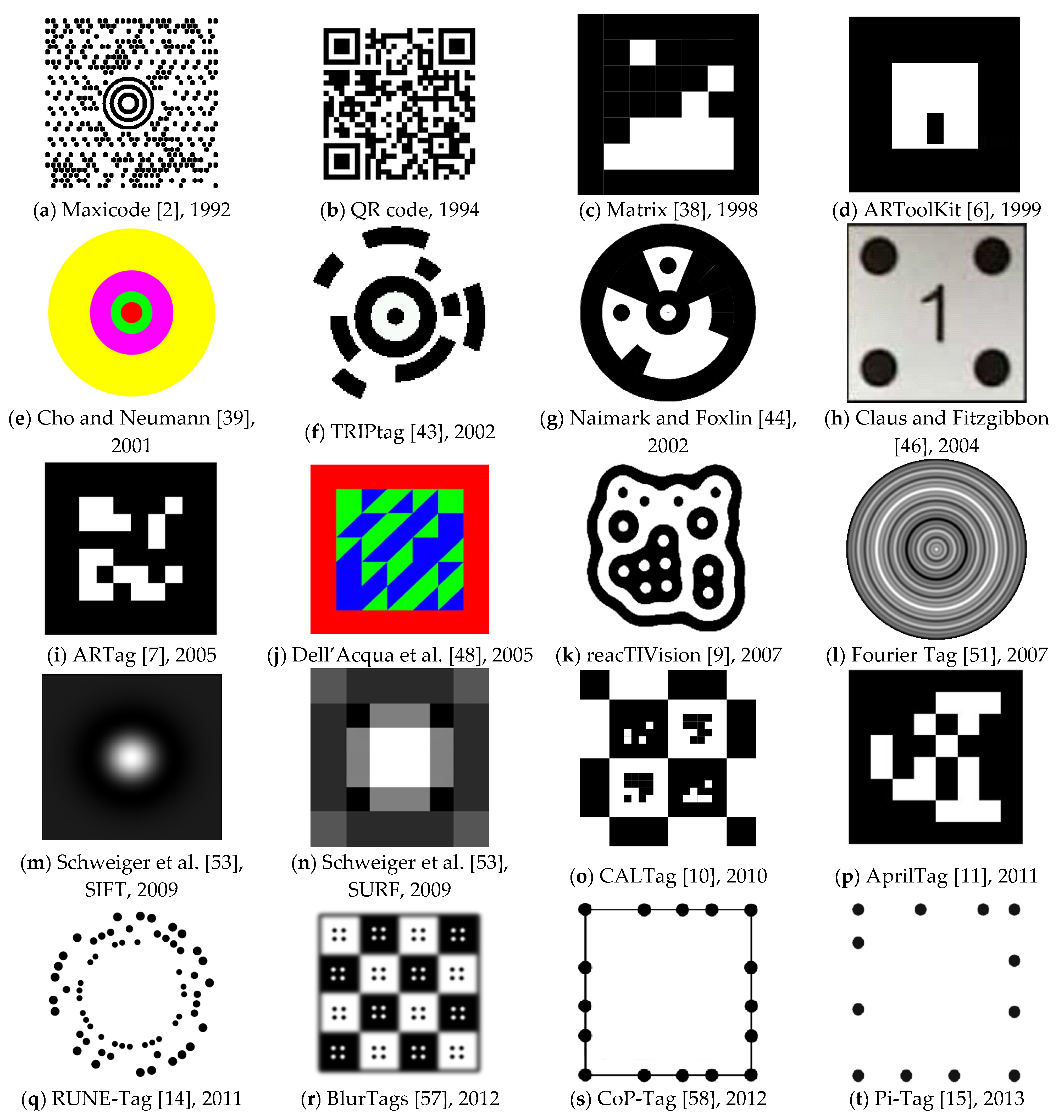
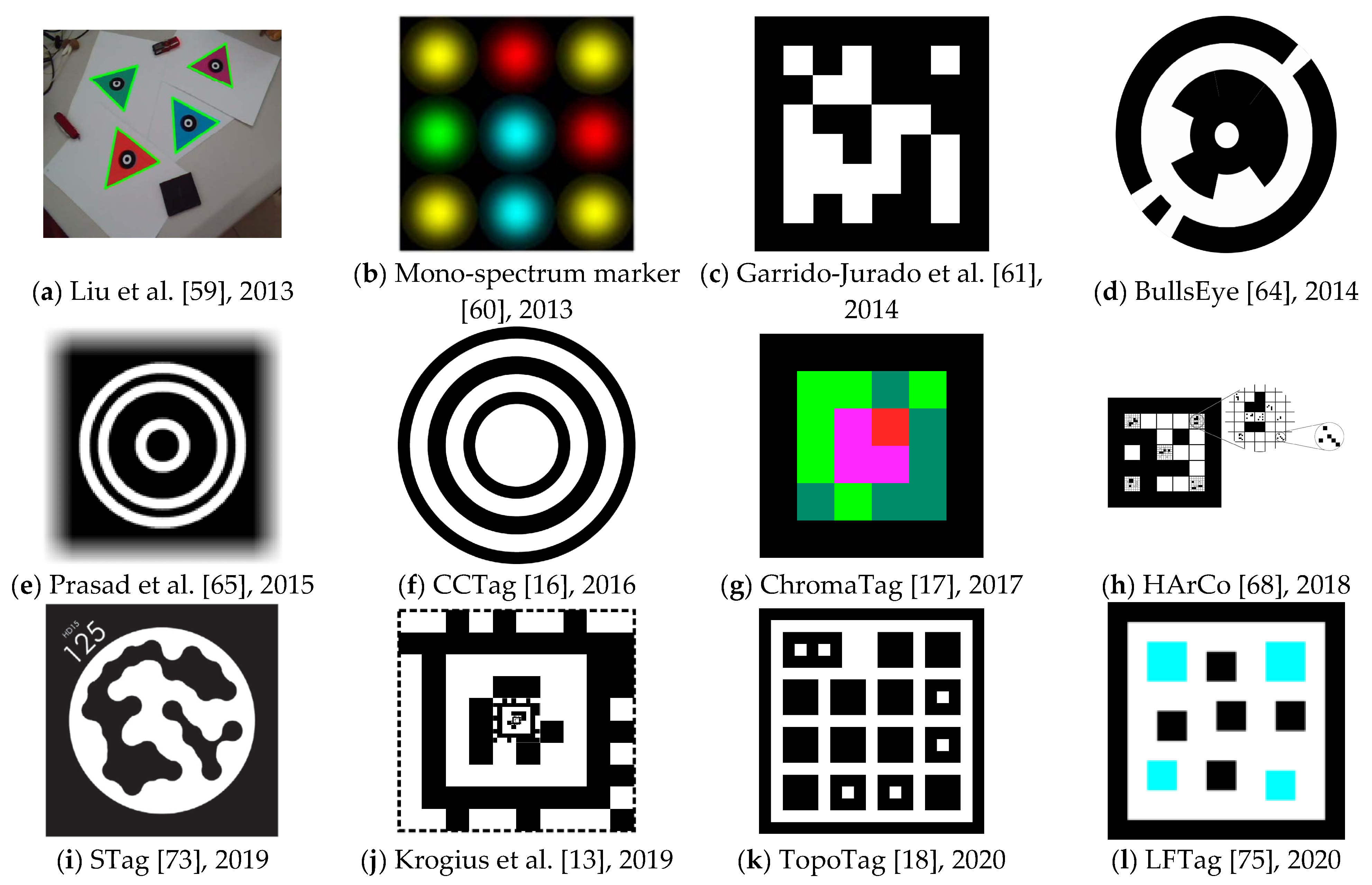
2. Related Work
- by the color of the marker
- ○
- black/grayscale (e.g., ARToolKit, ARTag, Fourier Tag)
- ○
- colored (e.g., ChromaTag, LFTag)
- by the shape of the marker
- ○
- square (e.g., ARTag, AprilTag, CALTag)
- ○
- circle (e.g., TRIPtag, RUNE-Tag)
- ○
- other (e.g., ReacTIVision)
- by the primary target application
- ○
- carry complex information (e.g., Maxicode, QR code)
- ○
- carry ID-based information (e.g., ARTag, April Tag)
- ○
- localization (e.g., SIFTtag, SURFtag)
- ○
- camera calibration or camera pose estimation (e.g., CALTag, HArCo)
Summary
3. Materials and Methods
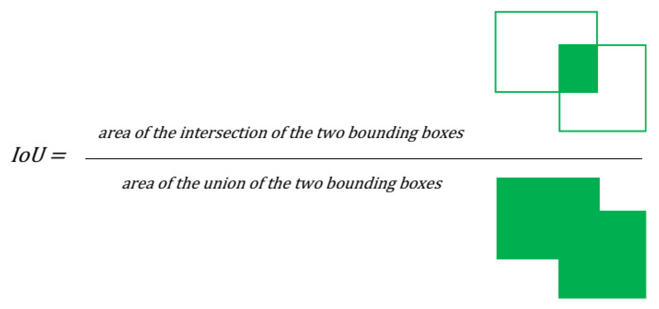
3.1. Methodology
- true positive cases (TP)—all markers that were correctly detected;
- false positive cases (FP)—all detected markers that do not correspond to any true marker;
- true negative cases (TN)—any detection algorithm can detect a virtually unlimited number of possible bounding boxes even in a single image; therefore, all places in an image that do not have any detected marker while there is no true marker are considered as true negatives; there can be an unlimited number of such bounding boxes, and we consider true negative count always zero—this limits the usage of some statistical metrics (e.g., accuracy, which would always be 1);
- false negative cases (FN)—all true markers that were not detected.
3.2. Theoretical Design
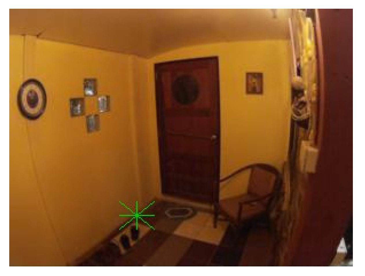
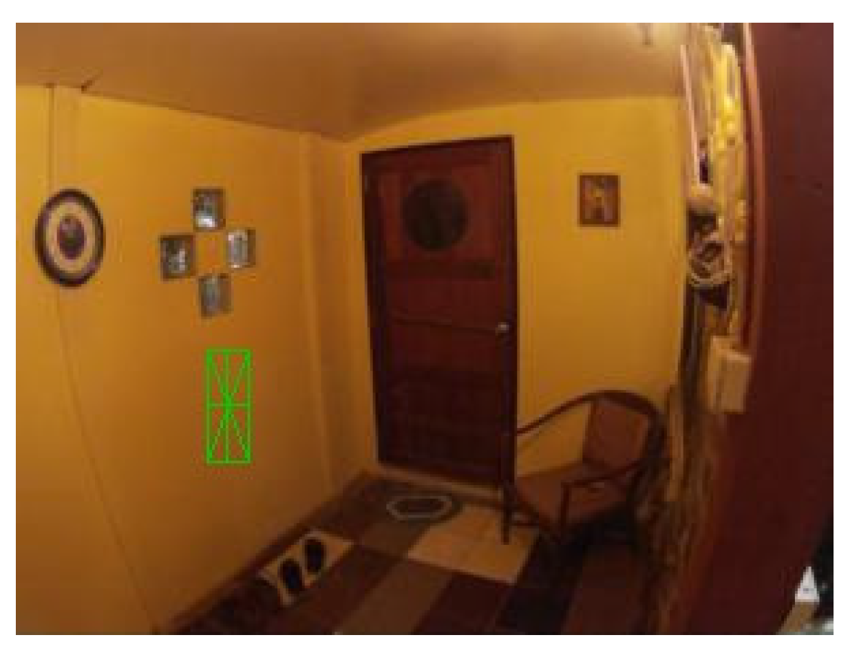
- localization of the marker (preferably its center);
- detection of rotation angle in 360° relative to the viewer;
- detection of the whole marker to obtain its relative size;
- and having a shape that supports obtaining of perspective transformation.
3.3. Dataset
3.4. Neural Network Architecture
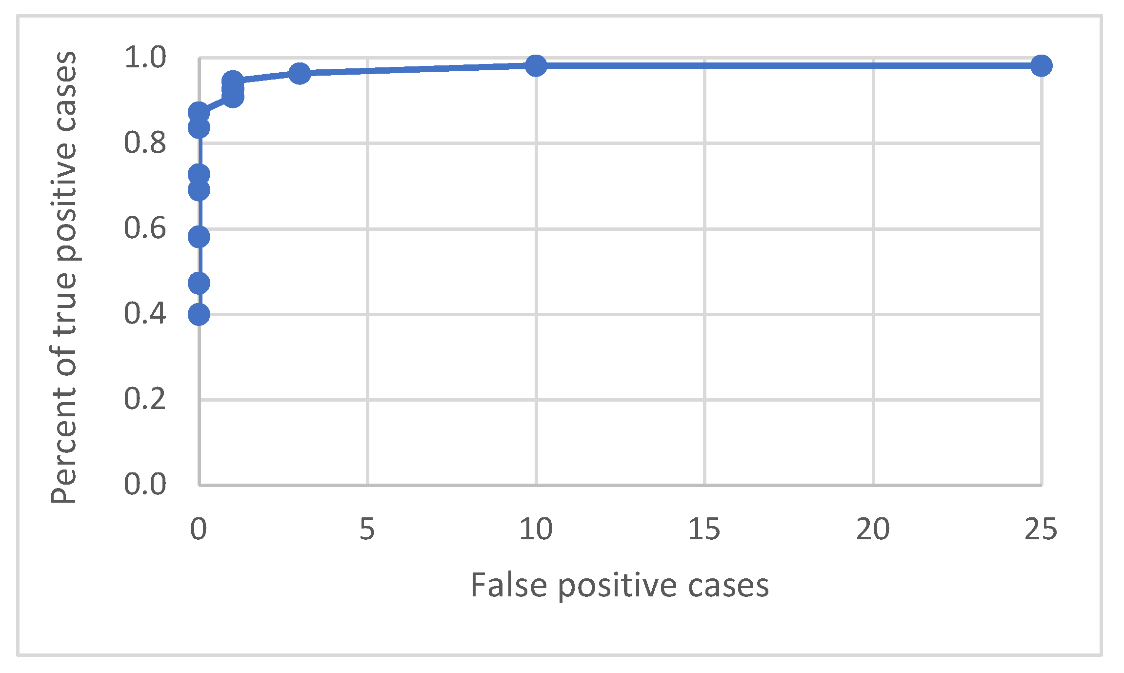
4. Results
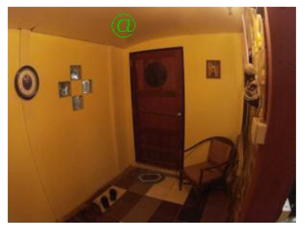
4.1. Initial Test Iterations
- filled rectangle;
- empty rectangle;
- filled triangle;
- empty triangle;
- star of thickness 2;
- star of thickness 1;
- star of thickness 1 surrounded by a rectangle;
- and @ symbol.
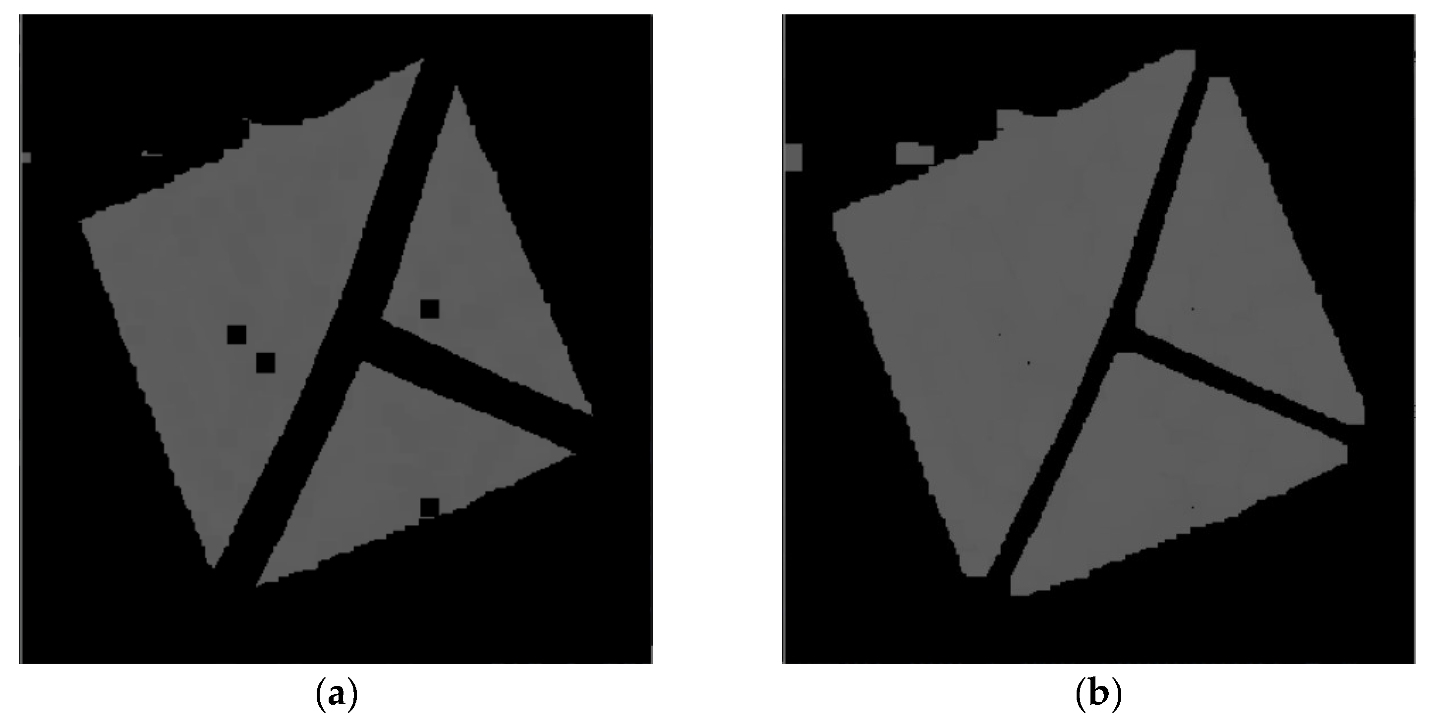
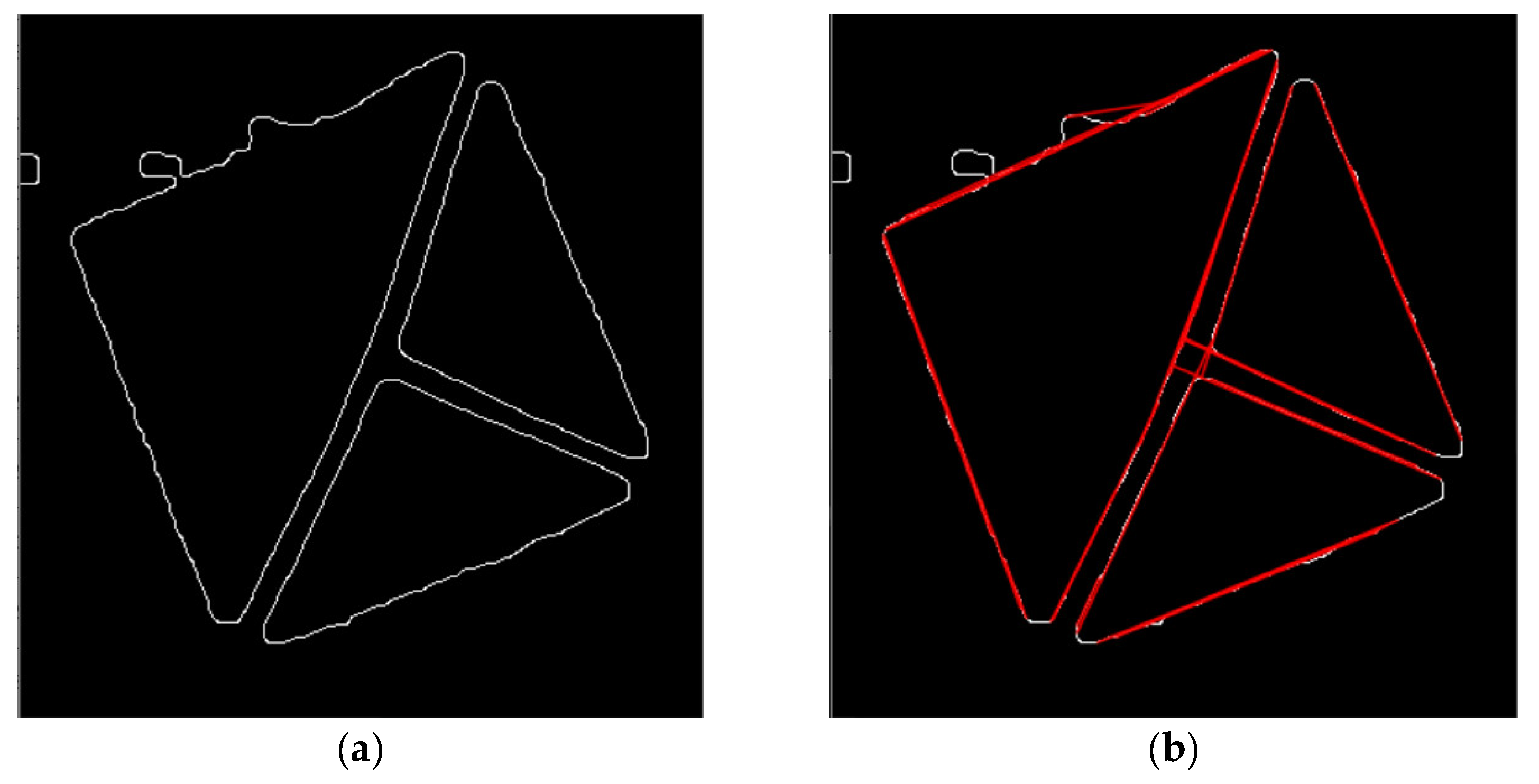
4.2. The “T cross” Shape
- Localization of the marker—the shape has a center to detect, and the center is detectable from the three lines going from the center to the three corners.
- Detection of rotation angle in 360° resolution relative to the viewer—the shape has three lines present in a way that allows detection of described rotation.
- Detection of the whole marker to obtain its relative size—the shape has a filled area that can be detected.
- Shape of the marker that supports obtaining perspective transformation—the shape has a filled area that can be used for this purpose.
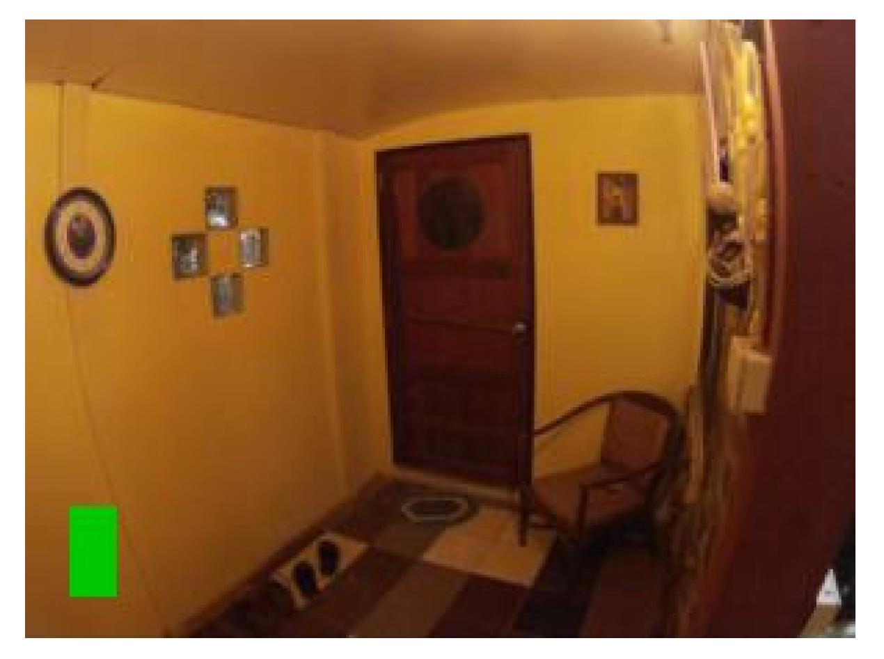
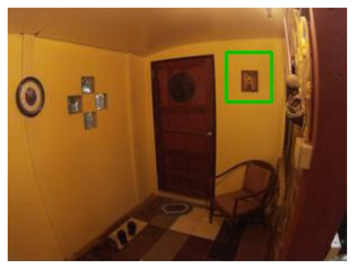
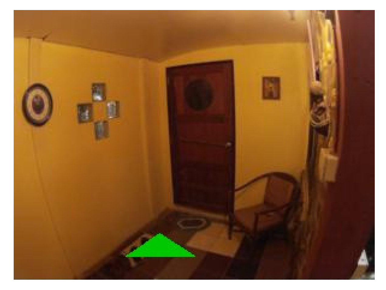
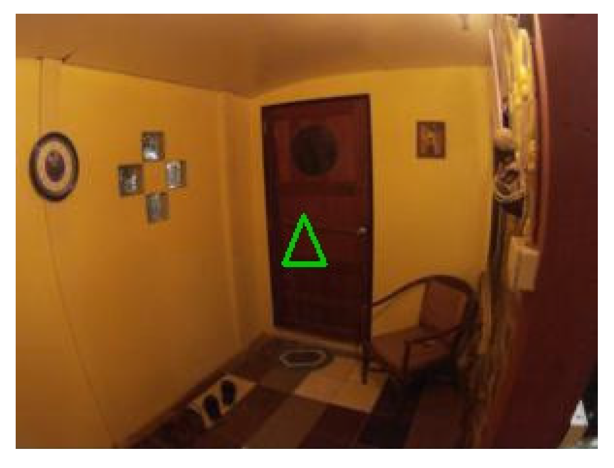
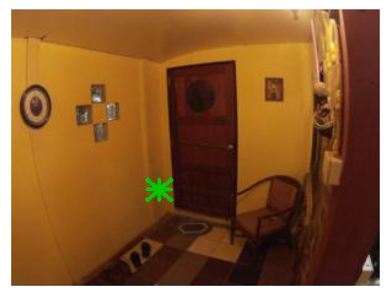
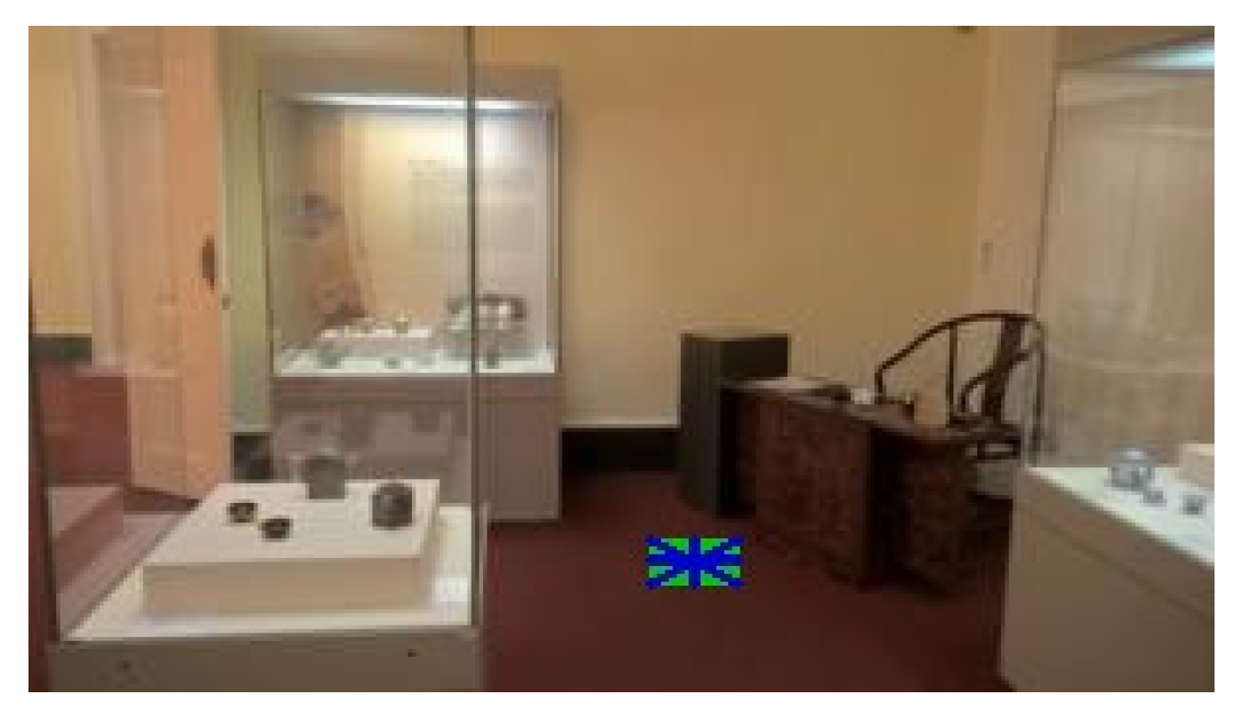
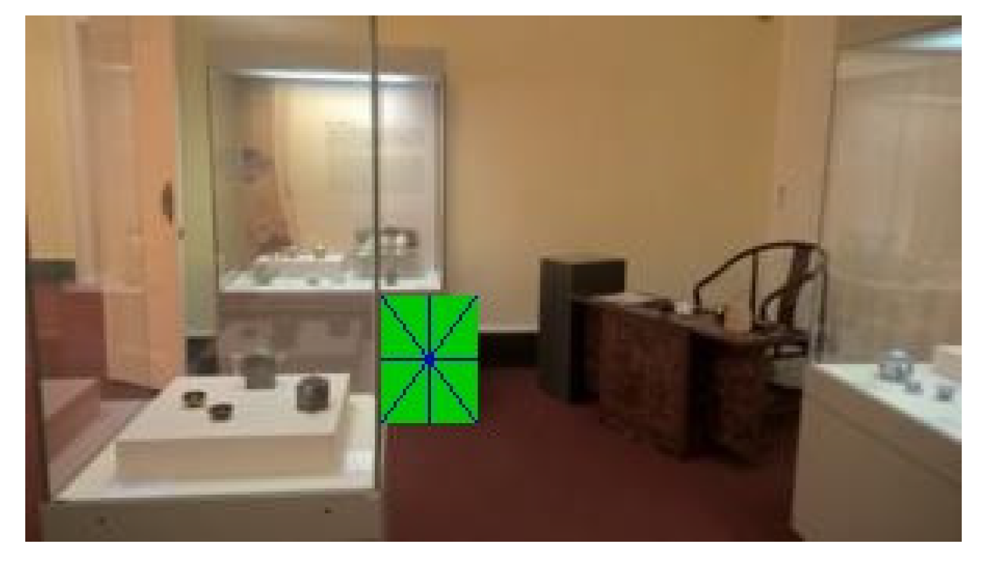
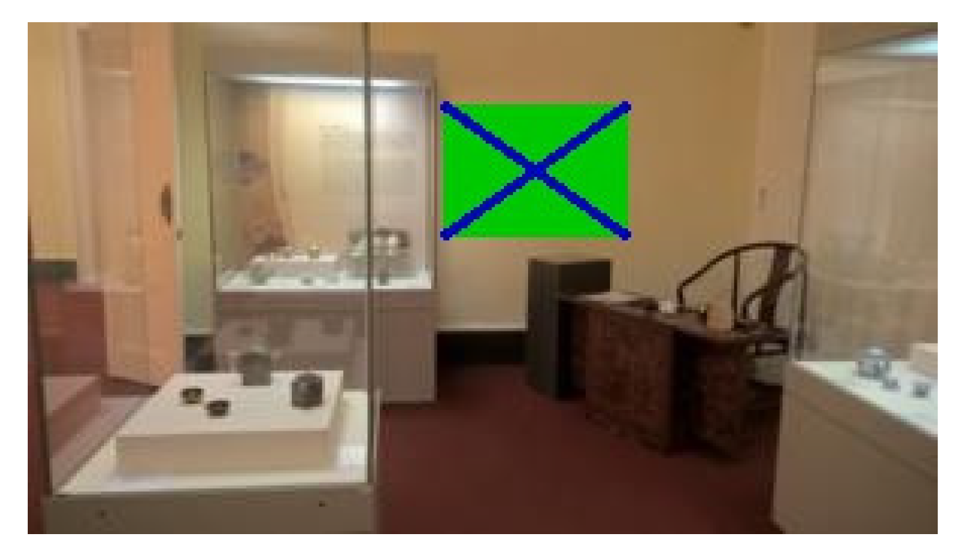
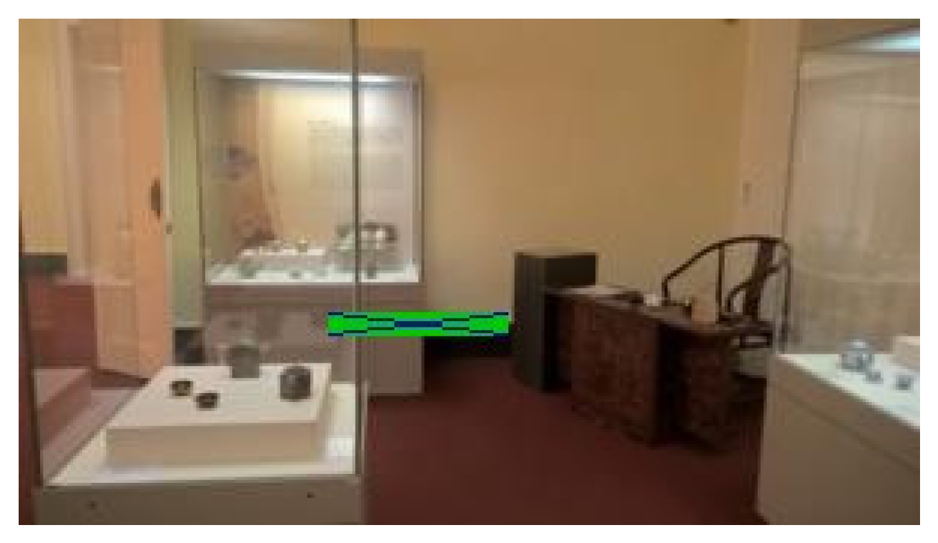
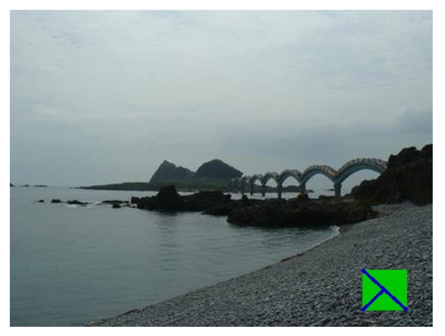
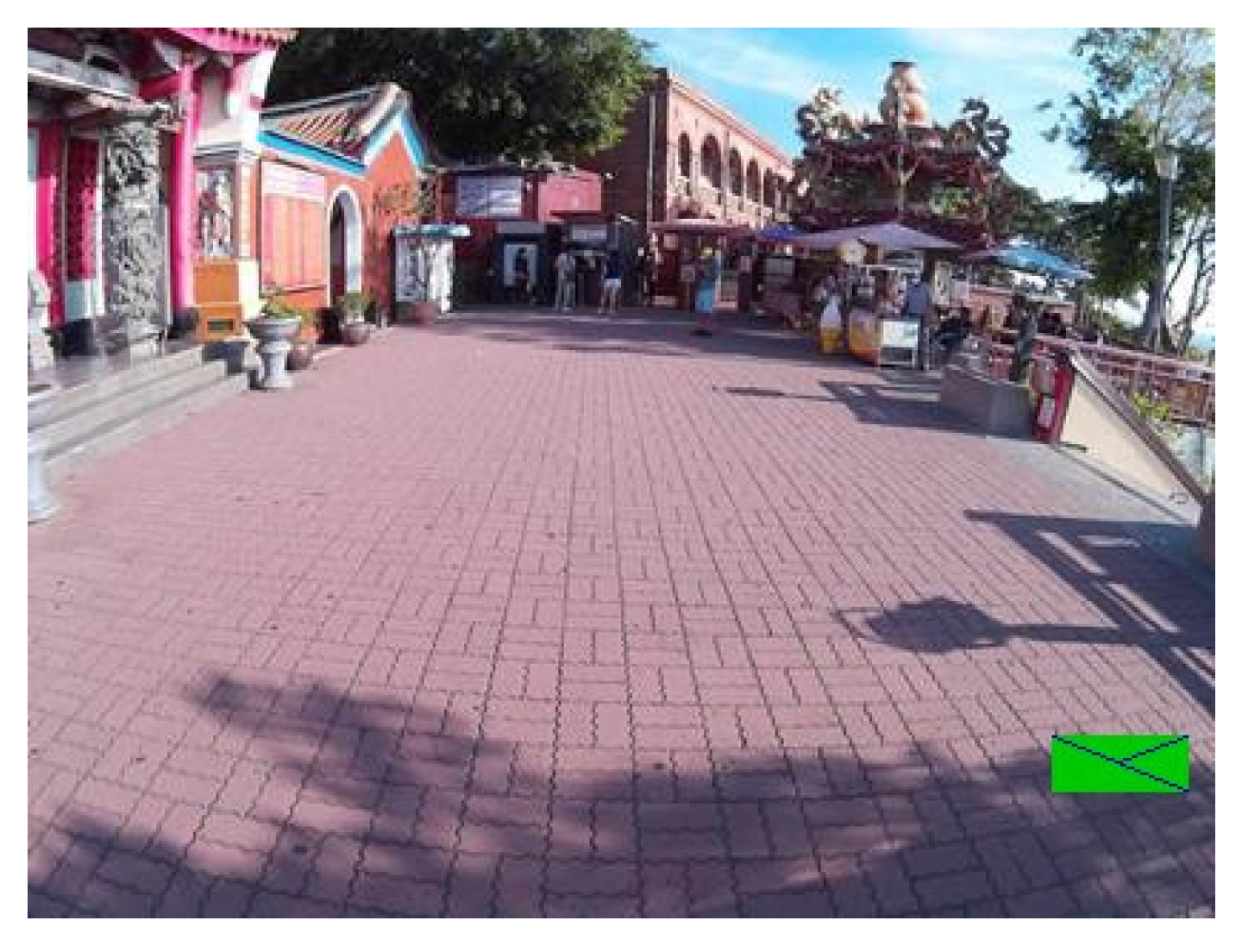
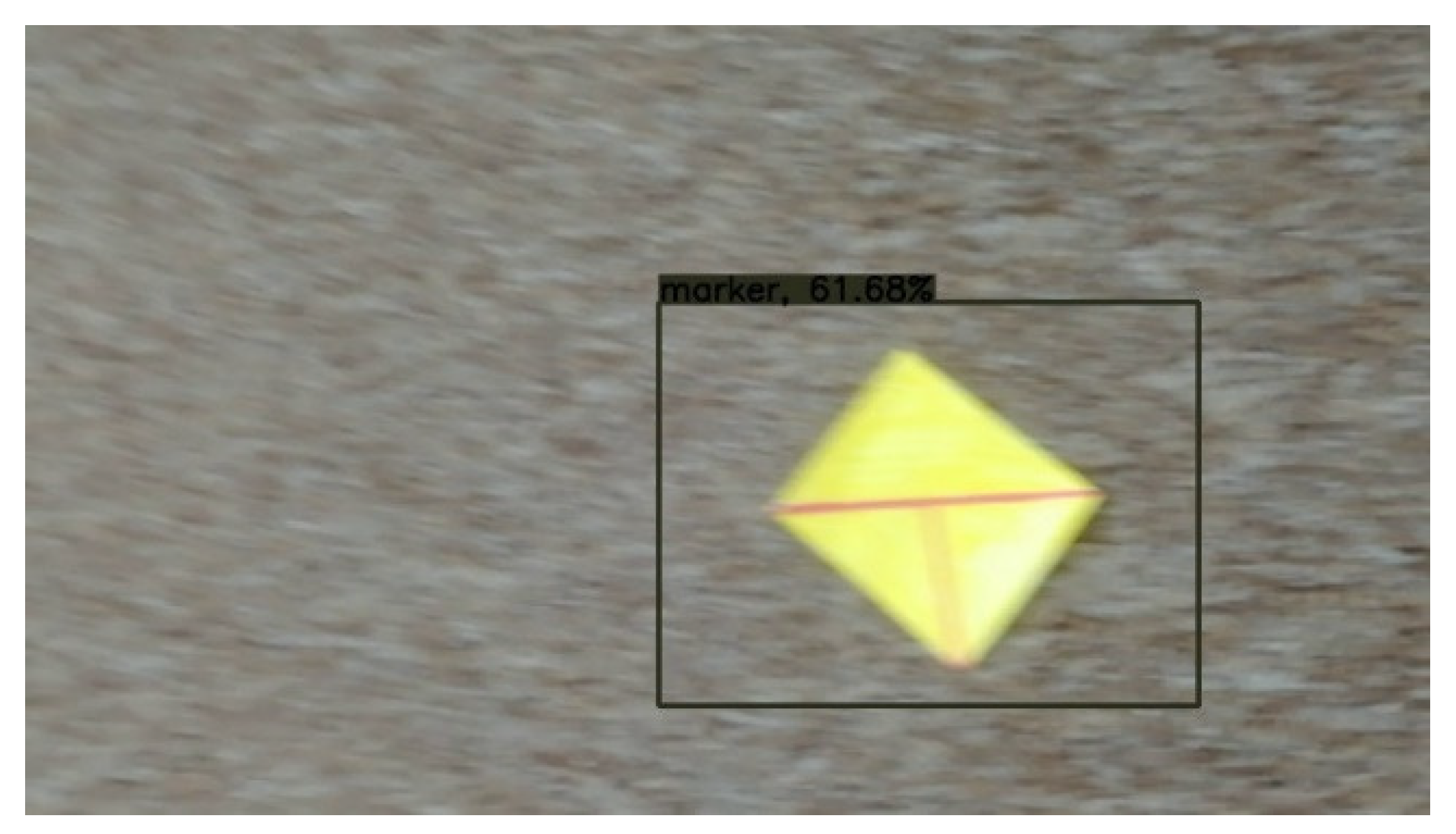
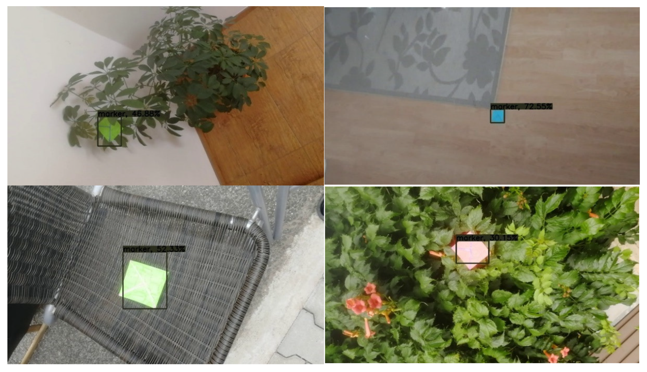
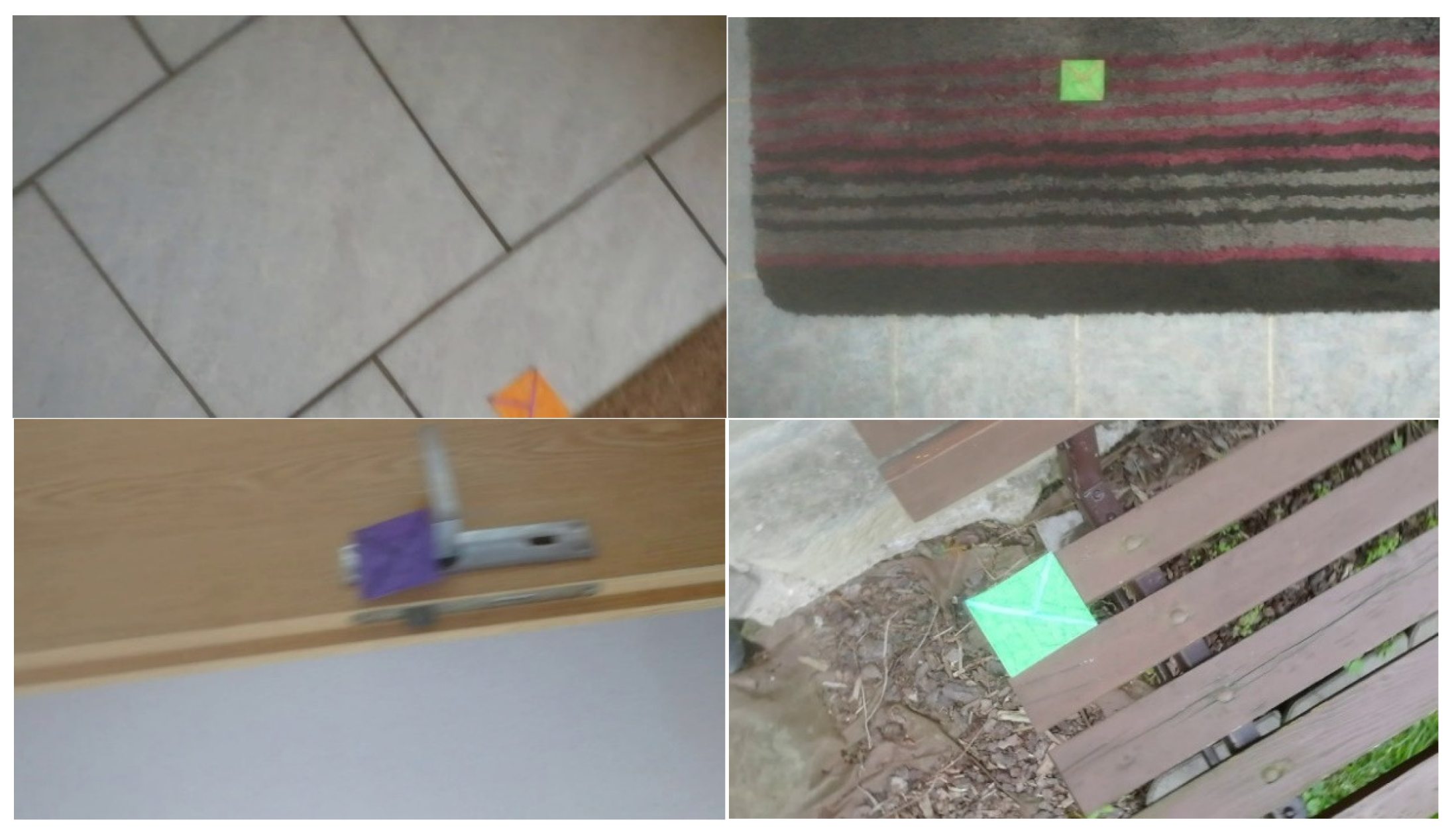
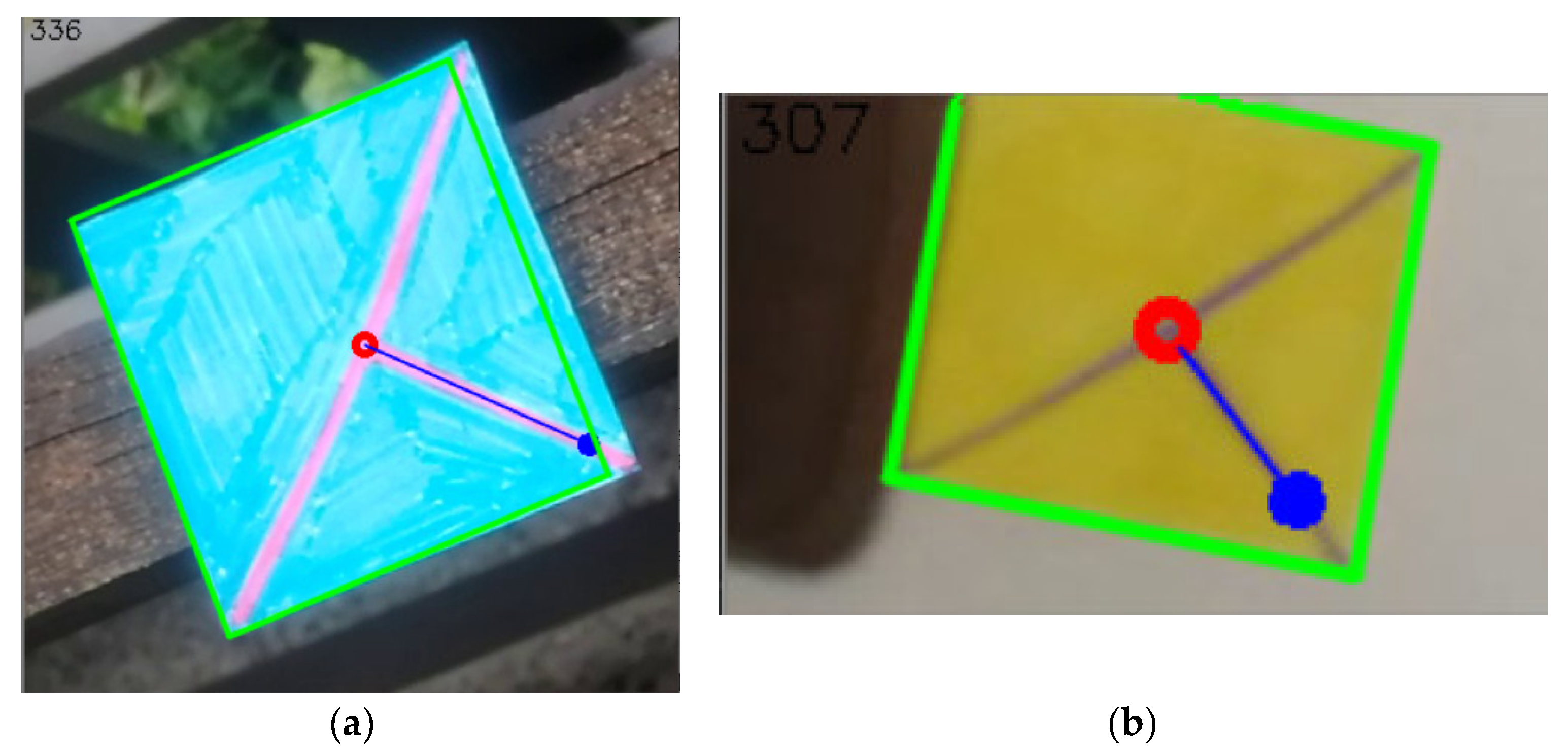
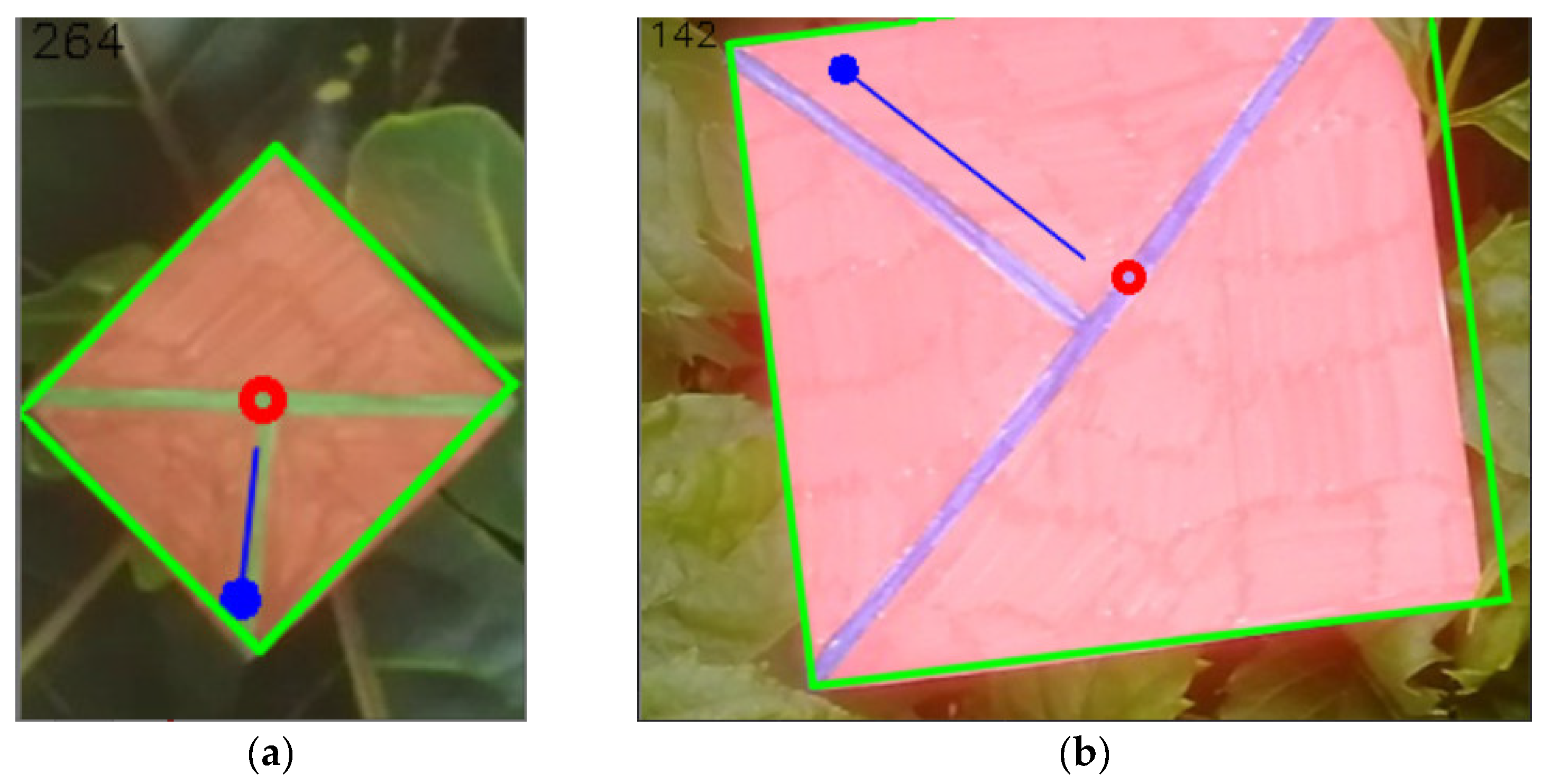
4.3. Markers in Real Scenes
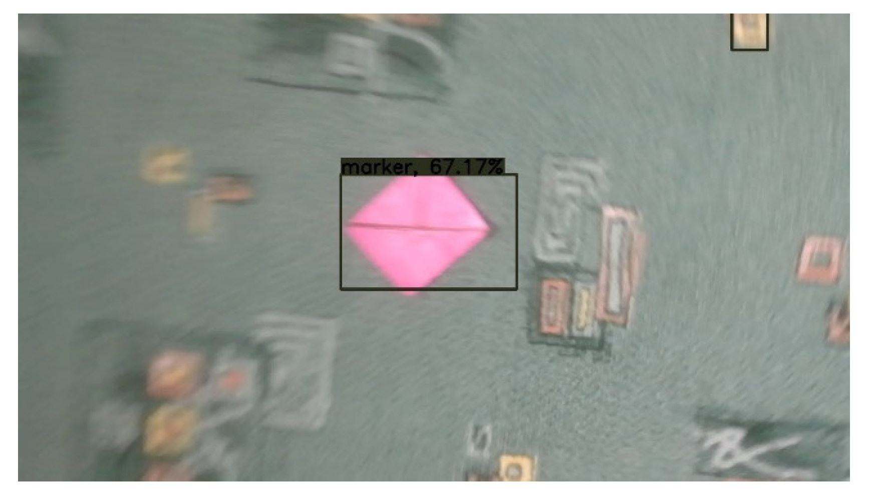
4.4. Examples of Detections of Real Markers
4.5. Summary of the Shape Design
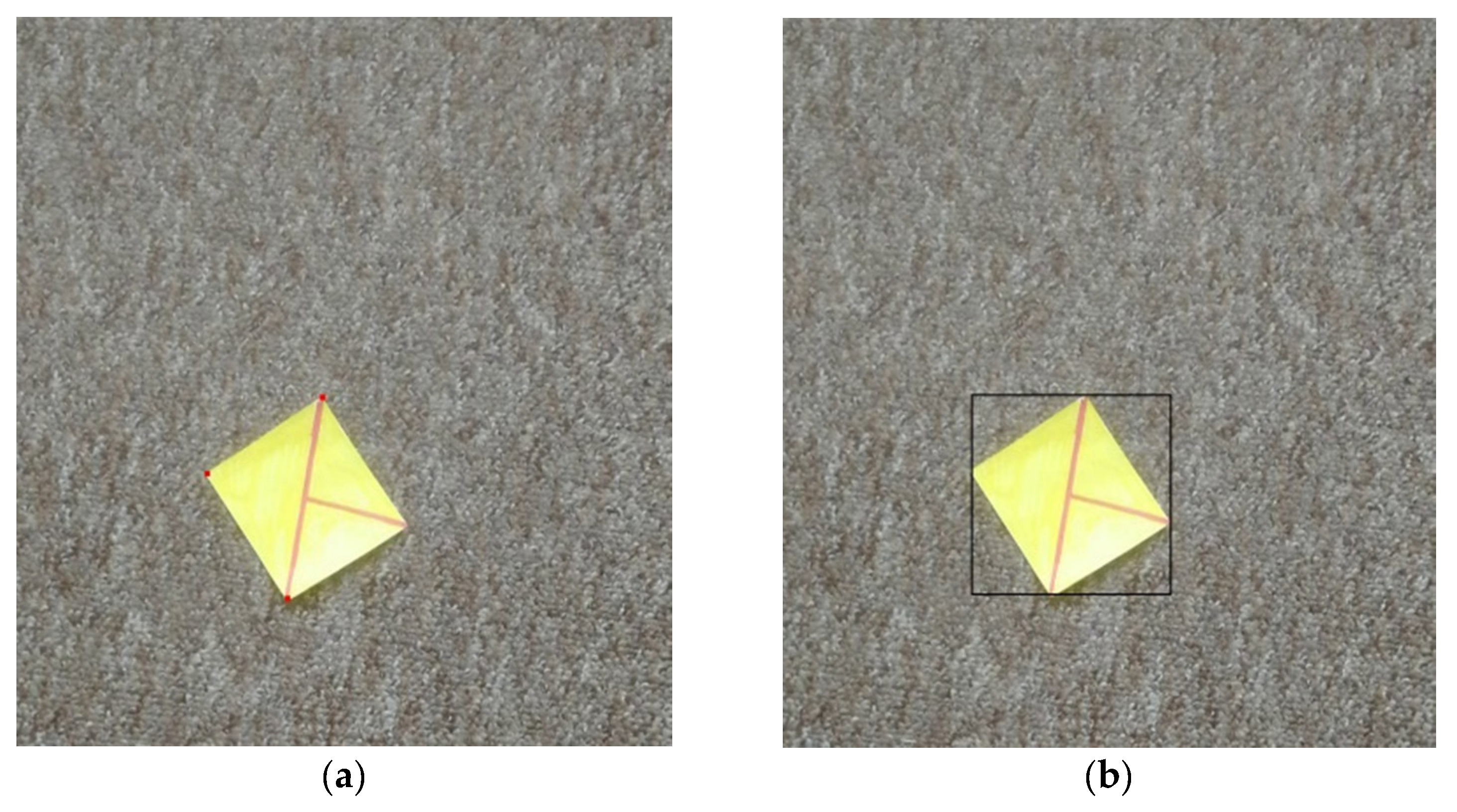
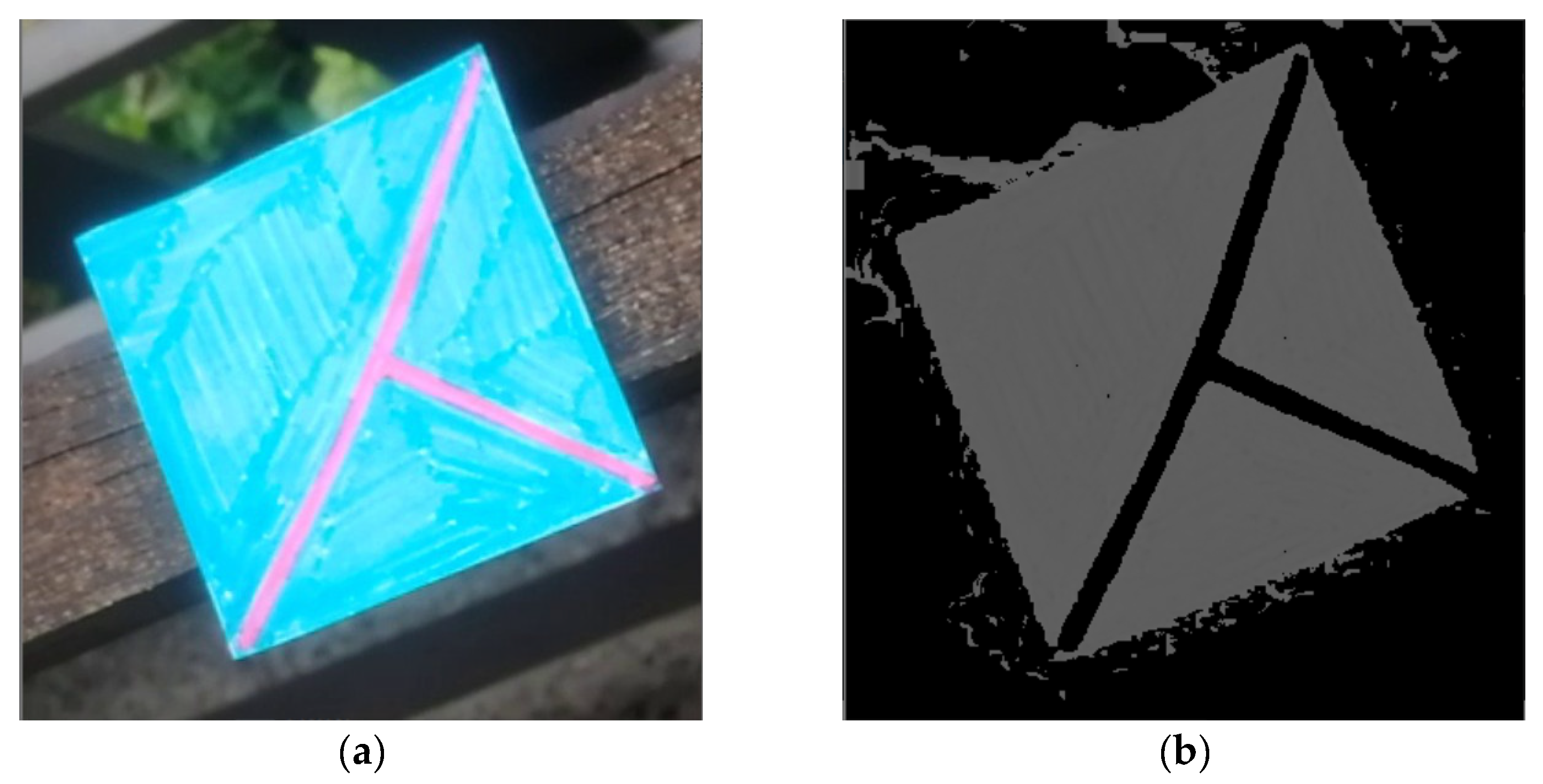
4.6. Getting Information from the Detected Marker
- 1)
- Crop the image with the detected coordinates and fixed padding.
- 2)
- Convert the image from the RGB to the HSV color model.
- 3)
- Build a histogram of hue values and get the hue with the largest count of pixels.
- 4)
- Filter out all other pixels with different hues.
- 5)
- Perform morphological operation erosion.
- 6)
- Perform morphological operation dilatation.
- 7)
- Apply Gaussian blur to the image.
- 8)
- Apply Otsu’s adaptive thresholding.
- 9)
- Apply Canny’s edge detector.
- 10)
- Apply Hough Lines algorithm.
4.7. Examples of the Information-Obtaining Process
5. Discussion
6. Conclusions
Author Contributions
Funding
Institutional Review Board Statement
Informed Consent Statement
Data Availability Statement
Conflicts of Interest
References
- ISO/IEC 18004:2015: Information Technology—Automatic Identification and Data Capture Techniques—QR Code Bar Code Symbology Specification. Available online: https://www.iso.org/cms/render/live/en/sites/isoorg/contents/data/standard/06/20/62021.html (accessed on 9 July 2020).
- Chandler, D.G.; Batterman, E.P.; Shah, G. Hexagonal, Information Encoding Article, Process and System. 1989. Available online: https://patents.google.com/patent/US4874936/en (accessed on 6 July 2020).
- Wang, Y.P.; Ye, A. Maxicode Data Extraction Using Spatial Domain Features. 1997. Available online: https://patents.google.com/patent/US5637849A/en (accessed on 12 August 2020).
- ISO/IEC 16023:2000: Information Technology—International Symbology Specification—MaxiCode. Available online: https://www.iso.org/cms/render/live/en/sites/isoorg/contents/data/standard/02/98/29835.html (accessed on 9 July 2020).
- KATO, H. ARToolKit: Library for Vision-based Augmented Reality. Tech. Rep. IEICE. PRMU 2002, 101, 79–86. [Google Scholar]
- Kato, H.; Billinghurst, M. Marker tracking and HMD calibration for a video-based augmented reality conferencing system. In Proceedings of the 2nd IEEE and ACM International Workshop on Augmented Reality (IWAR’99), San Francisco, CA, USA, 20–21 October 1999; pp. 85–94. [Google Scholar] [CrossRef] [Green Version]
- Fiala, M. ARTag, a Fiducial marker system using digital techniques. In Proceedings of the 2005 IEEE Computer Society Conference on Computer Vision and Pattern Recognition (CVPR’05), San Diego, CA, USA, 20–25 June 2005; Volume 2, pp. 590–596. [Google Scholar] [CrossRef]
- Fiala, M. Comparing ARTag and ARToolkit Plus fiducial marker systems. In Proceedings of the IEEE International Workshop on Haptic Audio Visual Environments and their Applications, Ottawa, ON, Canada, 1 October 2005; p. 6. [Google Scholar] [CrossRef]
- Kaltenbrunner, M.; Bencina, R. reacTIVision: A computer-vision framework for table-based tangible interaction. In Proceedings of the 1st International Conference on Tangible and Embedded Interaction-TEI ’07, New York, NY, USA, 15–17 February 2007; ACM Press: Baton Rouge, LO, USA, 2007; p. 69. [Google Scholar] [CrossRef]
- Koch, R.; Kolb, A.; Rezk-salama, C.; Atcheson, B.; Heide, F.; Heidrich, W. (Eds.) CALTag: High Precision Fiducial Markers for Camera Calibration; The Eurographics Association: Norrköping, Sweden, 2010. [Google Scholar]
- Olson, E. AprilTag: A robust and flexible visual fiducial system. In Proceedings of the 2011 IEEE International Conference on Robotics and Automation, Shanghai, China, 9–13 May 2011; pp. 3400–3407. [Google Scholar] [CrossRef] [Green Version]
- Wang, J.; Olson, E. AprilTag 2: Efficient and robust fiducial detection. In Proceedings of the 2016 IEEE/RSJ International Conference on Intelligent Robots and Systems (IROS), Daejeon, Korea, 9–14 October 2016; pp. 4193–4198. [Google Scholar] [CrossRef]
- Krogius, M.; Haggenmiller, A.; Olson, E. Flexible Layouts for Fiducial Tags. In Proceedings of the 2019 IEEE/RSJ International Conference on Intelligent Robots and Systems (IROS), Macau, China, 3–8 November 2019; pp. 1898–1903. [Google Scholar] [CrossRef]
- Bergamasco, F.; Albarelli, A.; Rodolà, E.; Torsello, A. RUNE-Tag: A high accuracy fiducial marker with strong occlusion resilience. In Proceedings of the CVPR 2011, Colorado Springs, CO, USA, 20–25 June 2011; pp. 113–120. [Google Scholar] [CrossRef] [Green Version]
- Bergamasco, F.; Albarelli, A.; Torsello, A. Pi-Tag: A fast image-space marker design based on projective invariants. Mach. Vis. Appl. 2013, 24, 1295–1310. [Google Scholar] [CrossRef] [Green Version]
- Calvet, L.; Gurdjos, P.; Griwodz, C.; Gasparini, S. Detection and accurate localization of circular fiducials under highly challenging conditions. In Proceedings of the 2016 IEEE Conference on Computer Vision and Pattern Recognition (CVPR), Las Vegas, NV, USA, 27–30 June 2016; pp. 562–570. [Google Scholar] [CrossRef] [Green Version]
- DeGol, J.; Bretl, T.; Hoiem, D. ChromaTag: A Colored Marker and Fast Detection Algorithm. In Proceedings of the 2017 IEEE International Conference on Computer Vision (ICCV), Venice, Italy, 22–29 October 2017; pp. 1481–1490. [Google Scholar] [CrossRef] [Green Version]
- Yu, G.; Hu, Y.; Dai, J. TopoTag: A robust and scalable topological fiducial marker system. IEEE Trans. Visual. Comput. Graph. 2020, 27, 1. [Google Scholar] [CrossRef] [Green Version]
- Fong, S.L.; Yung, D.C.W.; Ahmed, F.Y.H.; Jamal, A. Smart city bus application with Quick Response (QR) code payment. In Proceedings of the 2019 8th International Conference on Software and Computer Applications, New York, NY, USA, 19–21 February 2019; Association for Computing Machinery: New York, NY, USA, 2019; pp. 248–252. [Google Scholar] [CrossRef]
- Košt’ák, M.; Ježek, B. Mobile phone as an interactive device in augmented reality system. In Proceedings of the DIVAI 2018, Štúrovo, Slovakia, 2–4 May 2018. [Google Scholar]
- Košťák, M.; Ježek, B.; Slabý, A. Color marker detection with WebGL for mobile augmented reality systems. In Mobile Web and Intelligent Information Systems; Awan, I., Younas, M., Ünal, P., Aleksy, M., Eds.; Springer International Publishing: Cham, Switzerland, 2019; pp. 71–84. [Google Scholar] [CrossRef]
- Košťák, M.; Ježek, B.; Slabý, A. Adaptive detection of single-color marker with WebGL. In Augmented Reality, Virtual Reality, and Computer Graphics; De Paolis, L.T., Bourdot, P., Eds.; Springer International Publishing: Cham, Switzerland, 2020; pp. 395–410. [Google Scholar] [CrossRef]
- Dos Santos Cesar, D.B.; Gaudig, C.; Fritsche, M.; dos Reis, M.A.; Kirchner, F. An evaluation of artificial fiducial markers in underwater environments. In Proceedings of the OCEANS 2015-Genova IEEE, Genova, Italy, 18–21 May 2015; pp. 1–6. [Google Scholar] [CrossRef]
- Bondy, M.; Krishnasamy, R.; Crymble, D.; Jasiobedzki, P. Space Vision Marker System (SVMS). In Proceedings of the AIAA SPACE 2007 Conference & Exposition, Long Beach, CA, USA, 18—20 September 2007; American Institute of Aeronautics and Astronautics: Long Beach, CA, USA, 2007. [Google Scholar] [CrossRef]
- Zhang, X.; Fronz, S.; Navab, N. Visual marker detection and decoding in AR systems: A comparative study. In Proceedings of the International Symposium on Mixed and Augmented Reality, Darmstadt, Germany, 30 September–1 October 2002; pp. 97–106. [Google Scholar] [CrossRef]
- Shabalina, K.; Sagitov, A.; Sabirova, L.; Li, H.; Magid, E. ARTag, apriltag and caltag fiducial systems comparison in a presence of partial rotation: Manual and automated approaches. In Informatics in Control, Automation and Robotics; Gusikhin, O., Madani, K., Eds.; Lecture Notes in Electrical Engineering; Springer International Publishing: Cham, Switzerland, 2019; Volume 495, pp. 536–558. ISBN 978-3-030-11291-2. [Google Scholar] [CrossRef]
- Morar, A.; Moldoveanu, A.; Mocanu, I.; Moldoveanu, F.; Radoi, I.E.; Asavei, V.; Gradinaru, A.; Butean, A. A comprehensive survey of indoor localization methods based on computer vision. Sensors 2020, 20, 2641. [Google Scholar] [CrossRef] [PubMed]
- Owen, C.B.; Xiao, F.; Middlin, P. What is the best fiducial? In Proceedings of the The First IEEE International Workshop Agumented Reality Toolkit, Darmstadt, Germany, 29–29 September 2002; p. 8. [Google Scholar] [CrossRef]
- Fiala, M. Designing Highly Reliable Fiducial Markers. IEEE Trans. Pattern Anal. Mach. Intell. 2010, 32, 1317–1324. [Google Scholar] [CrossRef]
- Lowe, D.G. Object recognition from local scale-invariant features. In Proceedings of the Seventh IEEE International Conference on Computer Vision, Kerkyra, Greece, 20–27 September 1999; Volume 2, pp. 1150–1157. [Google Scholar] [CrossRef]
- Wagner, D.; Reitmayr, G.; Mulloni, A.; Drummond, T.; Schmalstieg, D. Real-time detection and tracking for augmented reality on mobile phones. IEEE Trans. Vis. Comput. Graph. 2010, 16, 355–368. [Google Scholar] [CrossRef] [PubMed]
- Gao, Q.H.; Wan, T.R.; Tang, W.; Chen, L. A Stable and accurate marker-less augmented reality registration method. In Proceedings of the 2017 International Conference on Cyberworlds (CW), Chester, UK, 20–22 September 2017; pp. 41–47. [Google Scholar] [CrossRef] [Green Version]
- Chen, C.-W.; Chen, W.-Z.; Peng, J.-W.; Cheng, B.-X.; Pan, T.-Y.; Kuo, H.-C. A Real-Time Markerless Augmented Reality Framework Based on SLAM Technique. In Proceedings of the 2017 14th International Symposium on Pervasive Systems, Algorithms and Networks 2017 11th International Conference on Frontier of Computer Science and Technology 2017 Third International Symposium of Creative Computing (ISPAN-FCST-ISCC), Exeter, UK, 21–23 June 2017; pp. 127–132. [Google Scholar] [CrossRef]
- Cheng, J.C.P.; Chen, K.; Chen, W. Comparison of Marker-Based and Markerless AR: A Case Study of An Indoor Decoration System. In Proceedings of the Lean and Computing in Construction Congress-Volume 1: Proceedings of the Joint Conference on Computing in Construction, Heraklion, Greece, 4–7 July 2017; Heriot-Watt University: Edinburgh, UK, 2017; pp. 483–490. [Google Scholar] [CrossRef] [Green Version]
- Brito, P.Q.; Stoyanova, J. Marker versus markerless augmented reality. Which has more impact on users? Int. J. Hum. Comput. Interact. 2018, 34, 819–833. [Google Scholar] [CrossRef]
- Gupta, A.; Bhatia, K.; Gupta, K.; Vardhan, M. A comparative study of marker-based and marker-less indoor navigation in augmented reality. Int. J. Eng. Res. Technol. 2018, 5, 4. [Google Scholar]
- Stridbar, L.; Henriksson, E. Subjective Evaluation of Marker-Based and Marker-Less AR for an Exhibition of a Digitally Recreated Swedish Warship; Blekinge Institute of Technology: Karlskrona, Sweden, 2019. [Google Scholar]
- Rekimoto, J. Matrix: A Realtime Object Identification and Registration Method for Augmented Reality. In Proceedings of the 3rd Asia Pacific Computer Human Interaction (Cat. No.98EX110), Shonan Village Center, Japan, 17 July 1998. [Google Scholar]
- Cho, Y.; Neumann, U. Multiring fiducial systems for scalable fiducial-tracking augmented reality. Presence 2001, 10, 599–612. [Google Scholar] [CrossRef]
- Zhang, X.; Genc, Y.; Navab, N. Taking AR into large scale industrial environments: Navigation and information access with mobile computers. In Proceedings of the IEEE and ACM International Symposium on Augmented Reality, New York, NY, USA, 29–30 October 2001; pp. 179–180. [Google Scholar] [CrossRef] [Green Version]
- Zhang, X.; Genc, Y.; Navab, N. Mobile computing and industrial augmented reality for real-time data access. In Proceedings of the ETFA 2001. 8th International Conference on Emerging Technologies and Factory Automation. Proceedings (Cat. No. 01TH8597), Antibes-Juan les Pins, France, 15–18 October 2001; Volume 2, pp. 583–588. [Google Scholar] [CrossRef]
- Appel, M.; Navab, N. Registration of technical drawings and calibrated images for industrial augmented reality. Mach. Vis. Appl. 2002, 13, 111–118. [Google Scholar] [CrossRef]
- López de Ipiña, D.; Mendonça, P.R.S.; Hopper, A.; Hopper, A. TRIP: A low-cost vision-based location system for ubiquitous computing. Pers. Ubiquitous Comput. 2002, 6, 206–219. [Google Scholar] [CrossRef]
- Naimark, L.; Foxlin, E. Circular data matrix fiducial system and robust image processing for a wearable vision-inertial self-tracker. In Proceedings of the International Symposium on Mixed and Augmented Reality, Darmstadt, Germany, 1 October 2002; pp. 27–36. [Google Scholar] [CrossRef]
- Naimark, L.; Foxlin, E. Fiducial Detection System. 2007. Available online: https://patents.google.com/patent/US7231063B2/en (accessed on 18 July 2020).
- Claus, D.; Fitzgibbon, A.W. Reliable fiducial detection in natural scenes. In Computer Vision-ECCV 2004; Pajdla, T., Matas, J., Eds.; Lecture Notes in Computer Science; Springer: Berlin/Heidelberg, Germany, 2004; Volume 3024, pp. 469–480. [Google Scholar] [CrossRef]
- Claus, D.; Fitzgibbon, A.W. Reliable automatic calibration of a marker-based position tracking system. In Proceedings of the 2005 Seventh IEEE Workshops on Applications of Computer Vision (WACV/MOTION’05), Breckenridge, CO, USA, 5–7 January 2005; Volume 1, pp. 300–305. [Google Scholar] [CrossRef]
- Dell’Acqua, A.; Ferrari, M.; Marcon, M.; Sarti, A.; Tubaro, S. Colored visual tags: A robust approach for augmented reality. In Proceedings of the IEEE Conference on Advanced Video and Signal Based Surveillance, Como, Italy, 15–16 September 2005; pp. 423–427. [Google Scholar] [CrossRef]
- Kawano, T.; Ban, Y.; Uehara, K. A coded visual marker for video tracking system based on structured image analysis. In Proceedings of the The Second IEEE and ACM International Symposium on Mixed and Augmented Reality, Tokyo, Japan, 10 October 2003; pp. 262–263. [Google Scholar] [CrossRef]
- reacTIVision. Available online: https://sourceforge.net/projects/reactivision/ (accessed on 8 August 2020).
- Sattar, J.; Bourque, E.; Giguere, P.; Dudek, G. Fourier tags: Smoothly degradable fiducial markers for use in human-robot interaction. In Proceedings of the Fourth Canadian Conference on Computer and Robot Vision (CRV ’07), Montreal, QC, Canada, 28–30 May 2007; pp. 165–174. [Google Scholar] [CrossRef]
- Xu, A.; Dudek, G. Fourier Tag: A Smoothly degradable fiducial marker system with configurable payload capacity. In Proceedings of the 2011 Canadian Conference on Computer and Robot Vision, St. Johns, NL, Canada, 25–27 May 2011; pp. 40–47. [Google Scholar] [CrossRef]
- Schweiger, F.; Zeisl, B.; Georgel, P.; Schroth, G.; Steinbach, E.; Navab, N. Maximum detector response markers for SIFT and SURF. VMV 2009, 10, 145–154. [Google Scholar]
- Bay, H.; Tuytelaars, T.; Van Gool, L. SURF: Speeded up robust features. In Computer Vision–ECCV 2006; Leonardis, A., Bischof, H., Pinz, A., Eds.; Springer: Berlin/Heidelberg, Germany, 2006; pp. 404–417. [Google Scholar] [CrossRef]
- AprilTag. Available online: https://april.eecs.umich.edu/software/apriltag.html (accessed on 8 August 2020).
- Bergamasco, F.; Albarelli, A.; Cosmo, L.; Rodolà, E.; Torsello, A. An Accurate and Robust Artificial Marker Based on Cyclic Codes. IEEE Trans. Pattern Anal. Mach. Intell. 2016, 38, 2359–2373. [Google Scholar] [CrossRef] [PubMed] [Green Version]
- Reuter, A.; Seidel, H.-P.; Ihrke, I. BlurTags: Spatially Varying PSF Estimation with Out-of-Focus Patterns. In Proceedings of the 20th International Conference on Computer Graphics, Visualization and Computer Vision 2012, WSCG’2012, Plenz, Czech Republic, 26–28 June 2012; pp. 239–247. [Google Scholar]
- Li, Y.; Chen, Y.; Lu, R.; Ma, D.; Li, Q. A novel marker system in augmented reality. In Proceedings of the 2012 2nd International Conference on Computer Science and Network Technology, Changchun, China, 1 February 2012; pp. 1413–1417. [Google Scholar] [CrossRef]
- Liu, J.; Chen, S.; Sun, H.; Qin, Y.; Wang, X. Real Time Tracking Method by Using Color Markers. In Proceedings of the 2013 International Conference on Virtual Reality and Visualization, Washington, DC, USA, 14–15 September 2013; pp. 106–111. [Google Scholar] [CrossRef]
- Toyoura, M.; Aruga, H.; Turk, M.; Mao, X. Detecting Markers in Blurred and Defocused Images. In Proceedings of the 2013 International Conference on Cyberworlds, Yokohama, Japan, 21–23 October 2013; pp. 183–190. [Google Scholar] [CrossRef]
- Garrido-Jurado, S.; Muñoz-Salinas, R.; Madrid-Cuevas, F.J.; Marín-Jiménez, M.J. Automatic generation and detection of highly reliable fiducial markers under occlusion. Pattern Recognit. 2014, 47, 2280–2292. [Google Scholar] [CrossRef]
- ArUco: A Minimal Library for Augmented Reality Applications based on OpenCV|Aplicaciones de la Visión Artificial. Available online: http://www.uco.es/investiga/grupos/ava/node/26 (accessed on 9 August 2020).
- Garrido-Jurado, S.; Muñoz-Salinas, R.; Madrid-Cuevas, F.J.; Medina-Carnicer, R. Generation of fiducial marker dictionaries using Mixed Integer Linear Programming. Pattern Recognit. 2016, 51, 481–491. [Google Scholar] [CrossRef]
- Klokmose, C.N.; Kristensen, J.B.; Bagge, R.; Halskov, K. BullsEye: High-Precision Fiducial Tracking for Table-based Tangible Interaction. In Proceedings of the the Ninth ACM International Conference on Interactive Tabletops and Surfaces, New York, NY, USA, 16–19 November, 2014; Association for Computing Machinery: New York, NY, USA, 2014; pp. 269–278. [Google Scholar] [CrossRef] [Green Version]
- Prasad, M.G.; Chandran, S.; Brown, M.S. A motion blur resilient fiducial for quadcopter imaging. In Proceedings of the 2015 IEEE Winter Conference on Applications of Computer Vision, Waikoloa Beach, HI, USA, 6–8 July 2015; pp. 254–261. [Google Scholar] [CrossRef]
- CCTag. Available online: https://github.com/alicevision/CCTag (accessed on 8 August 2020).
- Calvet, L.; Gurdjos, P.; Charvillat, V. Camera tracking using concentric circle esmarkers: Paradigms and algorithms. In Proceedings of the 2012 19th IEEE International Conference on Image Processing, Washington, DC, USA, 24–29 July 2012; pp. 1361–1364. [Google Scholar] [CrossRef]
- Wang, H.; Shi, Z.; Lu, G.; Zhong, Y. Hierarchical fiducial marker design for pose estimation in large-scale scenarios. J. Field Robot. 2018, 35, 835–849. [Google Scholar] [CrossRef]
- Tateno, K.; Kitahara, I.; Ohta, Y. A nested marker for augmented reality. In Proceedings of the 2007 IEEE Virtual Reality Conference, Charlotte, NC, USA, 10–14 March 2007; pp. 259–262. [Google Scholar] [CrossRef]
- Romero-Ramirez, F.J.; Muñoz-Salinas, R.; Medina-Carnicer, R. Fractal Markers: A New Approach for Long-Range Marker Pose Estimation Under Occlusion. IEEE Access 2019, 7, 169908–169919. [Google Scholar] [CrossRef]
- Susan, S.; Tandon, S.; Seth, S.; Mudassir, M.T.; Chaudhary, R.; Baisoya, N. Kullback-Leibler Divergence based Marker Detection in Augmented Reality. In Proceedings of the 2018 4th International Conference on Computing Communication and Automation (ICCCA), Greater Noida, India, 14–15 December 2018; pp. 1–5. [Google Scholar] [CrossRef]
- Kullback, S.; Leibler, R.A. On information and sufficiency. Ann. Math. Statist. 1951, 22, 79–86. [Google Scholar] [CrossRef]
- Benligiray, B.; Topal, C.; Akinlar, C. STag: A stable fiducial marker system. Image Vis. Comput. 2019, 89, 158–169. [Google Scholar] [CrossRef] [Green Version]
- Benligiray, B. STag. Available online: https://github.com/bbenligiray/stag (accessed on 8 August 2020).
- Wang, B. LFTag: A scalable visual fiducial system with low spatial frequency. arXiv 2020, arXiv:2006.00842. [Google Scholar]
- Wang, B. Kingoflolz/Fiducial. Available online: https://github.com/kingoflolz/fiducial (accessed on 12 August 2020).
- Redmon, J.; Farhadi, A. YOLOv3: An Incremental Improvement. arXiv 2018, arXiv:1804.02767. [Google Scholar]
- Li, C.; Wang, R.; Li, J.; Fei, L. Face Detection Based on YOLOv3. In Recent Trends in Intelligent Computing, Communication and Devices; Jain, V., Patnaik, S., Popențiu Vlădicescu, F., Sethi, I.K., Eds.; Springer: Singapore, 2020; pp. 277–284. [Google Scholar] [CrossRef]
- Liu, G.; Nouaze, J.C.; Touko Mbouembe, P.L.; Kim, J.H. YOLO-Tomato: A Robust algorithm for tomato detection based on YOLOv3. Sensors 2020, 20, 2145. [Google Scholar] [CrossRef] [PubMed] [Green Version]
- Jiao, Z.; Zhang, Y.; Xin, J.; Mu, L.; Yi, Y.; Liu, H.; Liu, D. A deep learning based forest fire detection approach using UAV and YOLOv3. In Proceedings of the 2019 1 st International Conference on Industrial Artificial Intelligence (IAI), Shenyang, China, 23–27 July 2019; pp. 1–5. [Google Scholar] [CrossRef]
- Zhang, H.; Qin, L.; Li, J.; Guo, Y.; Zhou, Y.; Zhang, J.; Xu, Z. Real-time detection method for small traffic signs based on Yolov3. IEEE Access 2020, 8, 64145–64156. [Google Scholar] [CrossRef]
- Papadopoulos, D.P.; Uijlings, J.R.R.; Keller, F.; Ferrari, V. Extreme clicking for efficient object annotation. arXiv 2017, arXiv:1708.02750. [Google Scholar]
- Goodfellow, I.; Pouget-Abadie, J.; Mirza, M.; Xu, B.; Warde-Farley, D.; Ozair, S.; Courville, A.; Bengio, Y. Generative Adversarial Nets. 9. Available online: https://papers.nips.cc/paper/2014/file/5ca3e9b122f61f8f06494c97b1afccf3-Paper.pdf (accessed on 8 August 2021).
- Yang, Z.; Xu, H.; Deng, J.; Loy, C.C.; Lau, W.C. Robust and fast decoding of high-capacity color QR codes for mobile applications. IEEE Trans. Image Process. 2018, 27, 6093–6108. [Google Scholar] [CrossRef] [PubMed]
- OpenCV: Cv::QRCodeDetector Class Reference. Available online: https://docs.opencv.org/4.5.1/de/dc3/classcv_1_1QRCodeDetector.html#a7290bd6a5d59b14a37979c3a14fbf394 (accessed on 31 May 2021).

| Authors [Reference] | Marker Name/Title | Year | Citations | Base Shape | Colors |
|---|---|---|---|---|---|
| - | IGD | 1990s | - | square | black |
| - | Maxicode | 1992 | - | square | black |
| - | QR code | 1994 | - | square | black |
| - | HOM | 1994 | - | square | black |
| Rekimoto | Matrix | 1998 | 459 | square | black |
| Kato | ARToolKit | 1999 | 3469 | square | black |
| Cho and Neumann | - | 2001 | 75 | circle | colors |
| - | SCR | 2001 | - | square | black |
| López de Ipiña et al. | TRIPtag | 2002 | 298 | circle | black |
| Naimark and Foxlin | - | 2002 | 387 | circle | black |
| Claus and Fitzgibbon | - | 2004, 2005 | 84 + 59 | square | black |
| Fiala | ARTag | 2005 | 1060 | square | black |
| Dell’Acqua et al. | - | 2005 | 10 | square | colors |
| Kaltenbrunner and Bencina | ReacTIVision | 2007 | 572 | other | black |
| Sattar et al. | Fourier Tag | 2007 | 66 | circle | grayscale |
| Flohr and Fischer | BinARyID | 2007 | 28 | square | black |
| Schweiger et al. | SIFTtag, SURFtag | 2009 | 31 | square | grayscale |
| Atcheson et al. | CALTag | 2010 | 130 | square | black |
| Xu and Dudek | Fourier Tag | 2011 | 31 | circle | grayscale |
| Olson | AprilTag | 2011 | 1085 | square | black |
| Bergamasco et al. | RUNE-Tag | 2011 | 117 | circle | black |
| Reuter et al. | BlurTags | 2012 | 8 | square | black |
| Li et al. | CoP-Tag | 2012 | 6 | square | black |
| Calvet et al. | C2Tag | 2012 | 23 | circle | black |
| Bergamasco et al. | Pi-Tag | 2013 | 60 | square | black |
| Liu et al. | - | 2013 | 11 | triangle | colors |
| Toyoura et al. | Mono-spectrum marker | 2013 | 17 | square | colors, black |
| Klokmose et al. | BullsEye | 2014 | 13 | circle | black |
| Garrido-Jurado et al. | ArUco | 2014, 2016 | 1389 + 329 | square | black |
| Prasad et al. | - | 2015 | 12 | circle | black |
| Wang and Olson | AprilTag 2 | 2016 | 340 | square | black |
| Calvet et al. | CCTag | 2016 | 43 | circle | black |
| DeGol et al. | ChromaTag | 2017 | 42 | square | colors, black |
| Wang et al. | HArCo | 2018 | 6 | square | black |
| Susan et al. | - | 2018 | 1 | square | black |
| Benligiray et al. | STag | 2019 | 9 | square | black |
| Krogius et al. | April Tag 3 | 2019 | 26 | square or circle | black |
| Yu et al. | TopoTag | 2020 | 7 | various | black |
| Marker Shape | Mean IoU | False Positive Cases | False Negative Cases | Percent of False Negative Cases | Precision | Recall |
|---|---|---|---|---|---|---|
| Filled rectangle | 0.665 | 15 | 16 | 5.4% | 0.949 | 0.946 |
| Empty rectangle | 0.666 | 12 | 16 | 5.4% | 0.959 | 0.946 |
| Filled triangle | 0.701 | 8 | 8 | 2.7% | 0.973 | 0.973 |
| Empty triangle | 0.679 | 6 | 13 | 4.4% | 0.979 | 0.956 |
| Star of thickness 2 | 0.695 | 3 | 9 | 3.0% | 0.990 | 0.970 |
| Star of thickness 1 | 0.654 | 13 | 19 | 6.4% | 0.955 | 0.936 |
| Star of thickness 1 surrounded by a rectangle | 0.614 | 19 | 21 | 7.1% | 0.936 | 0.929 |
| @ symbol | 0.699 | 10 | 19 | 6.4% | 0.965 | 0.936 |
| Marker Shape | Mean IoU | False Positive Cases | False Negative Cases | Percent of False Negative Cases | Precision | Recall |
|---|---|---|---|---|---|---|
| Star of thickness 2 in a filled rectangle | 0.755 | 2 | 9 | 1.9% | 0.996 | 0.981 |
| Star of thickness 1 in a filled rectangle | 0.764 | 7 | 11 | 2.3% | 0.985 | 0.977 |
| Cross of thickness 2 in a filled rectangle | 0.764 | 1 | 9 | 1.9% | 0.998 | 0.981 |
| Cross of thickness 1 in a filled rectangle | 0.764 | 3 | 5 | 1.0% | 0.994 | 0.990 |
| Marker Shape | Mean IoU | False Positive Cases | False Negative Cases | Percent of False Negative Cases | Precision | Recall |
|---|---|---|---|---|---|---|
| “T cross” of thickness 2 | 0.689 | 6 | 10 | 3.9% | 0.997 | 0.962 |
| “T cross” of thickness 1 | 0.664 | 5 | 13 | 5.0% | 0.980 | 0.950 |
| Marker Shape | Mean IoU | False Positive Cases | False Negative Cases | Percent of False Negative Cases | Precision | Recall |
|---|---|---|---|---|---|---|
| “T cross” of thickness 2 | 0.780 | 5 | 33 | 3.1% | 0.995 | 0.969 |
| “T cross” of thickness 1 | 0.743 | 10 | 62 | 5.8% | 0.990 | 0.943 |
| “T cross” of random thickness | 0.762 | 5 | 40 | 3.8% | 0.995 | 0.963 |
| Marker Shape | Detection Threshold | Mean IoU | True Positive Cases | False Positive Cases | False Negative Cases | Percent of False Negative Cases | Precision | Recall |
|---|---|---|---|---|---|---|---|---|
| T cross | 0.05 | 0.710 | 54 | 127 | 1 | 1.8% | 0.298 | 0.982 |
| 0.10 | 0.710 | 54 | 25 | 1 | 1.8% | 0.684 | 0.982 | |
| 0.15 | 0.707 | 54 | 10 | 1 | 1.8% | 0.844 | 0.982 | |
| 0.20 | 0.692 | 53 | 3 | 2 | 3.6% | 0.946 | 0.964 | |
| 0.25 | 0.685 | 52 | 1 | 3 | 5.5% | 0.981 | 0.945 | |
| 0.30 | 0.673 | 51 | 1 | 4 | 7.3% | 0.981 | 0.927 | |
| 0.35 | 0.659 | 50 | 1 | 5 | 9.1% | 0.980 | 0.909 | |
| 0.40 | 0.628 | 48 | 0 | 7 | 12.7% | 1.000 | 0.873 | |
| 0.45 | 0.600 | 46 | 0 | 9 | 16.4% | 1.000 | 0.836 | |
| 0.50 | 0.524 | 40 | 0 | 15 | 27.3% | 1.000 | 0.727 | |
| 0.55 | 0.501 | 38 | 0 | 17 | 30.9% | 1.000 | 0.691 | |
| 0.60 | 0.416 | 32 | 0 | 23 | 41.8% | 1.000 | 0.582 | |
| 0.65 | 0.332 | 26 | 0 | 29 | 52.7% | 1.000 | 0.473 | |
| 0.70 | 0.280 | 22 | 0 | 33 | 60.0% | 1.000 | 0.400 |
| Train Set | Mean IoU | False Positive Cases | False Negative Cases | Percent of False Negative Cases | Precision | Recall |
|---|---|---|---|---|---|---|
| Artificial (10,797 images) | 0.762 | 5 | 40 | 3.8% | 0.995 | 0.963 |
| Real (550 images) | 0.673 | 1 | 4 | 7.3% | 0.981 | 0.927 |
Publisher’s Note: MDPI stays neutral with regard to jurisdictional claims in published maps and institutional affiliations. |
© 2021 by the authors. Licensee MDPI, Basel, Switzerland. This article is an open access article distributed under the terms and conditions of the Creative Commons Attribution (CC BY) license (https://creativecommons.org/licenses/by/4.0/).
Share and Cite
Košťák, M.; Slabý, A. Designing a Simple Fiducial Marker for Localization in Spatial Scenes Using Neural Networks. Sensors 2021, 21, 5407. https://doi.org/10.3390/s21165407
Košťák M, Slabý A. Designing a Simple Fiducial Marker for Localization in Spatial Scenes Using Neural Networks. Sensors. 2021; 21(16):5407. https://doi.org/10.3390/s21165407
Chicago/Turabian StyleKošťák, Milan, and Antonín Slabý. 2021. "Designing a Simple Fiducial Marker for Localization in Spatial Scenes Using Neural Networks" Sensors 21, no. 16: 5407. https://doi.org/10.3390/s21165407
APA StyleKošťák, M., & Slabý, A. (2021). Designing a Simple Fiducial Marker for Localization in Spatial Scenes Using Neural Networks. Sensors, 21(16), 5407. https://doi.org/10.3390/s21165407