
A Flexible Baseline Measuring System Based on Optics for Airborne DPOS


Abstract
:1. Introduction
2. System Overview and External Parameter Calibration Method for Two Cameras with Non-Overlapping Fields of View
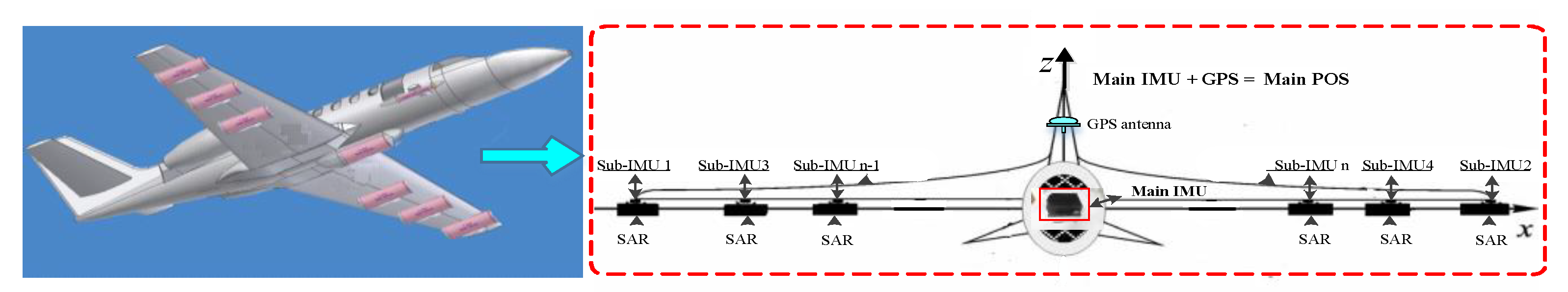
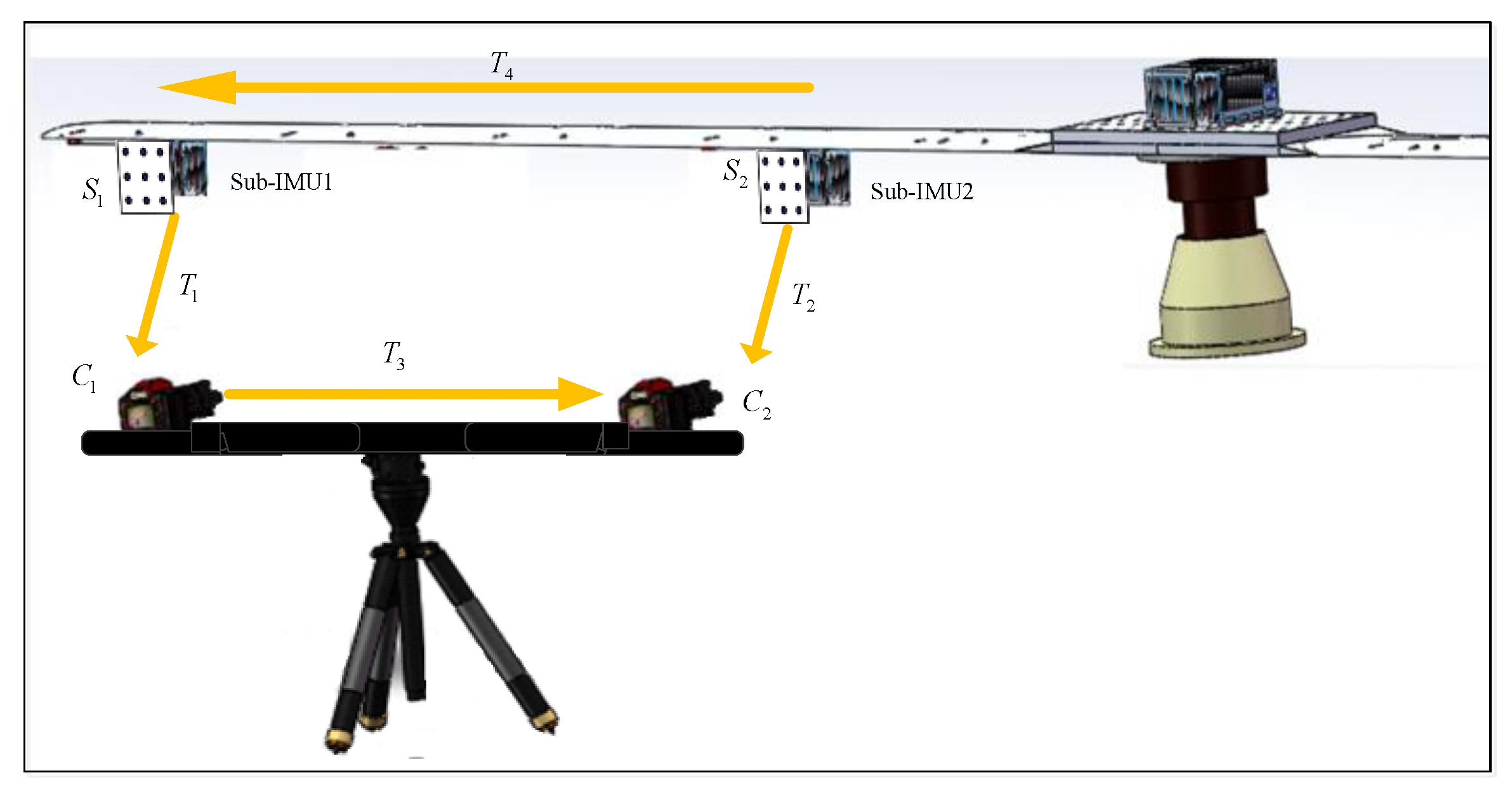
2.1. System Overview
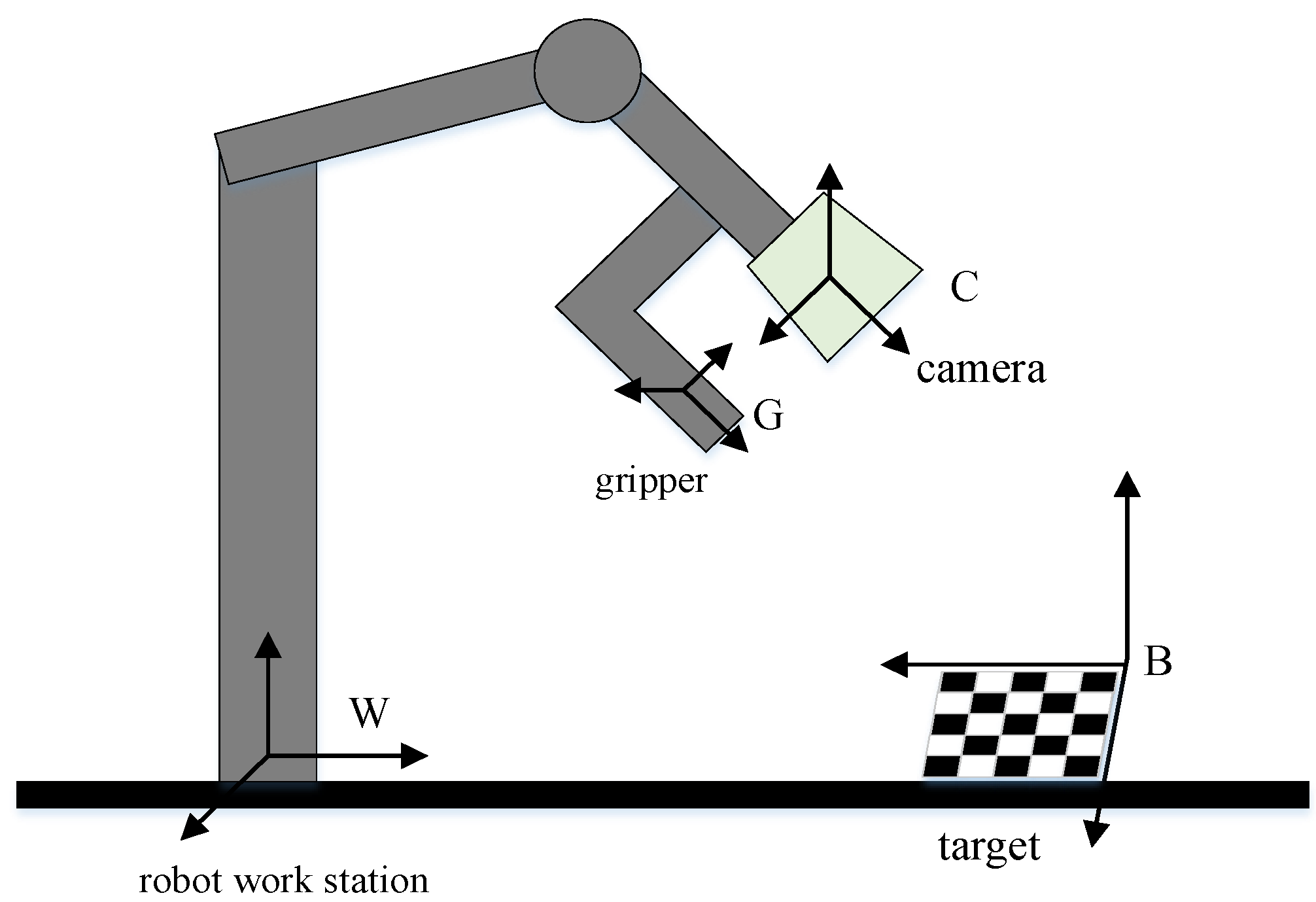
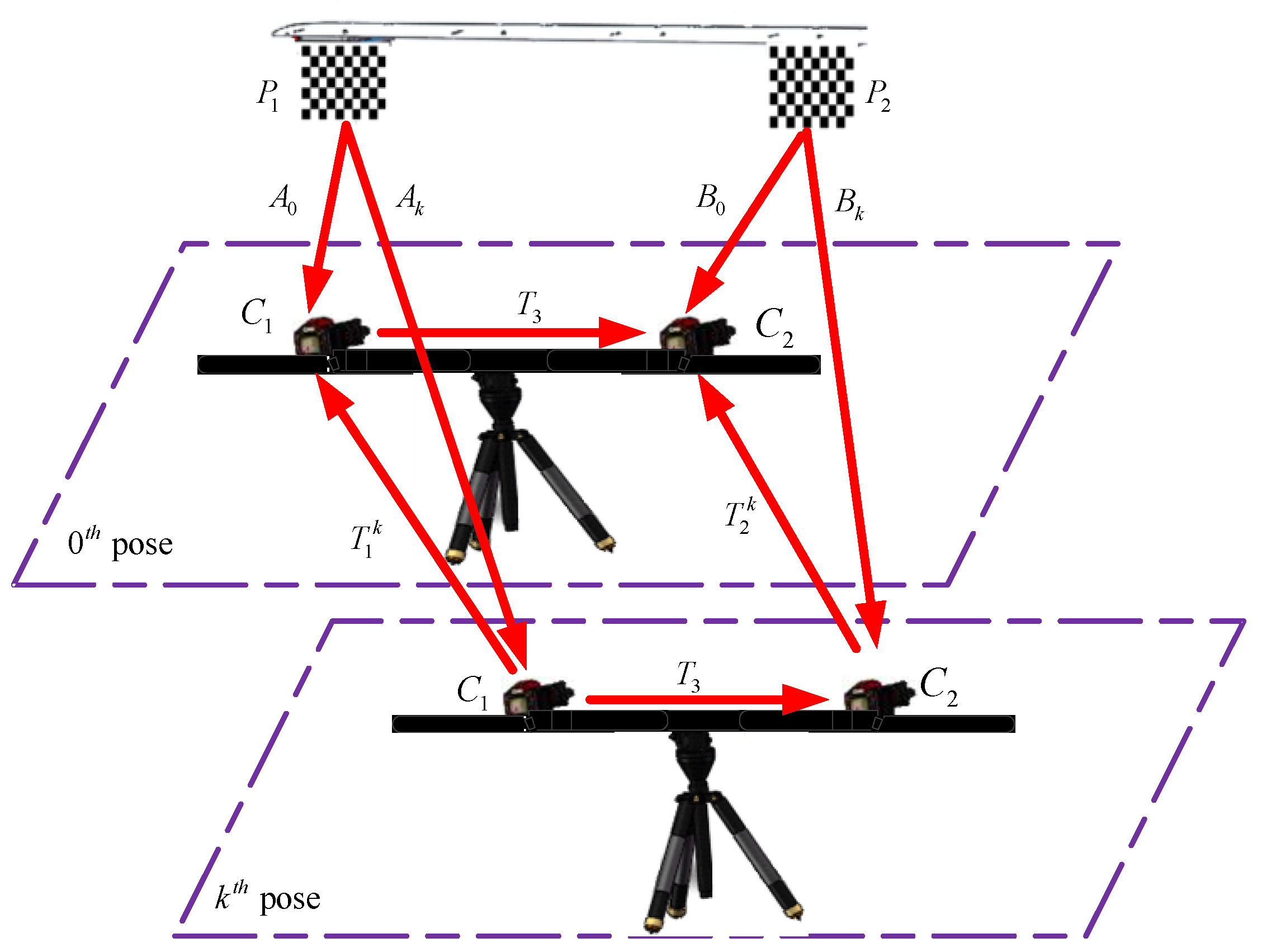
2.2. External Parameter Calibration Method for the Two Cameras with Non-Overlapping Fields of View
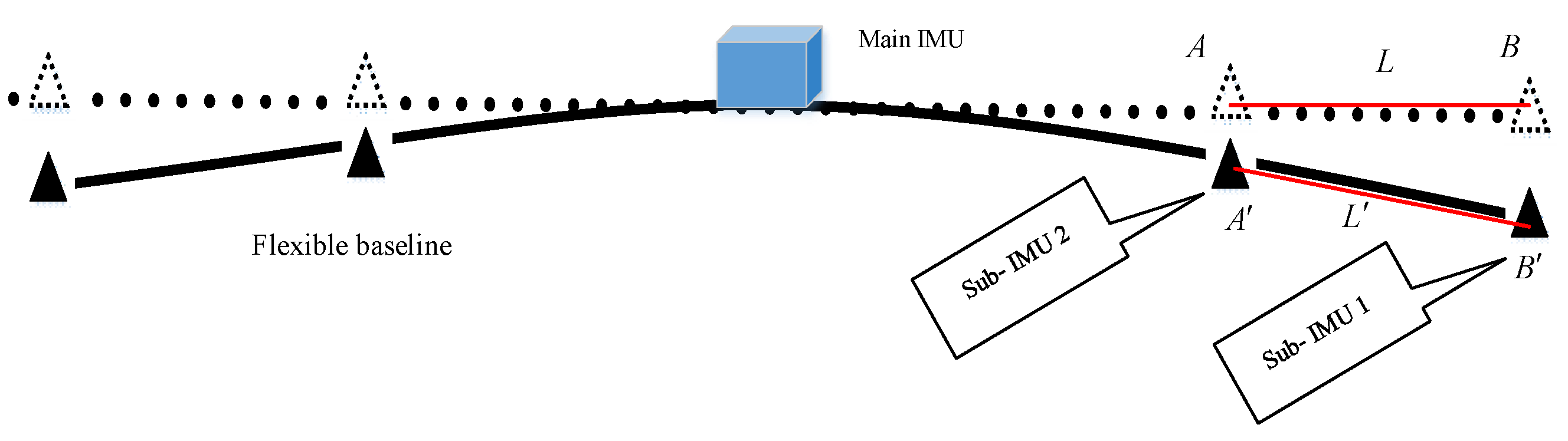
3. Flexible Baseline Measurement
4. Laboratory Tests for Flexible Baseline Measurement
4.1. External Parameter Calibration Method for the Two Cameras ()
4.1.1. DPOS Demonstration Platform
4.1.2. Cameras
4.2. Flexible Baseline Measurement
4.2.1. Static Test
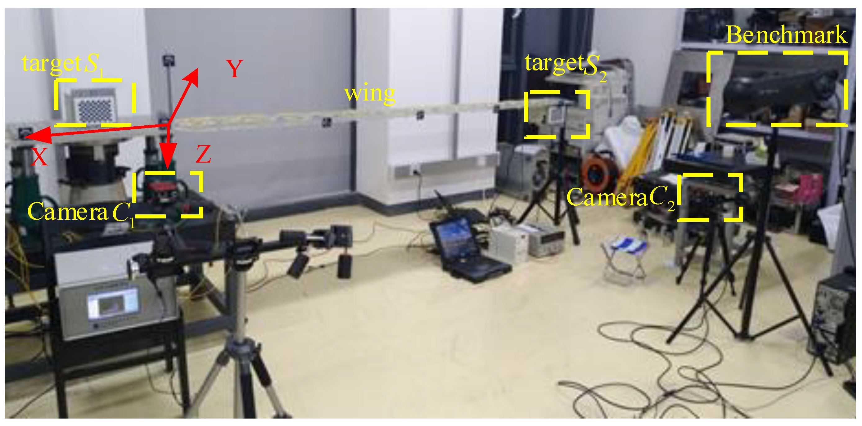
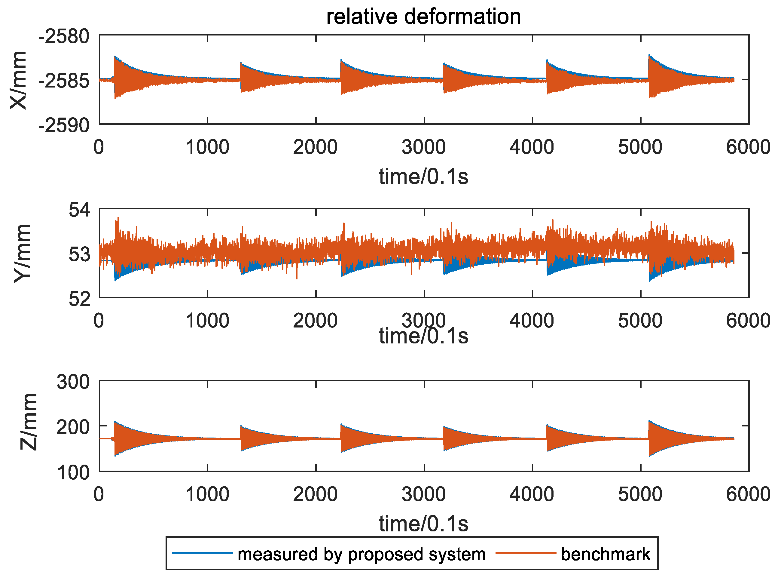
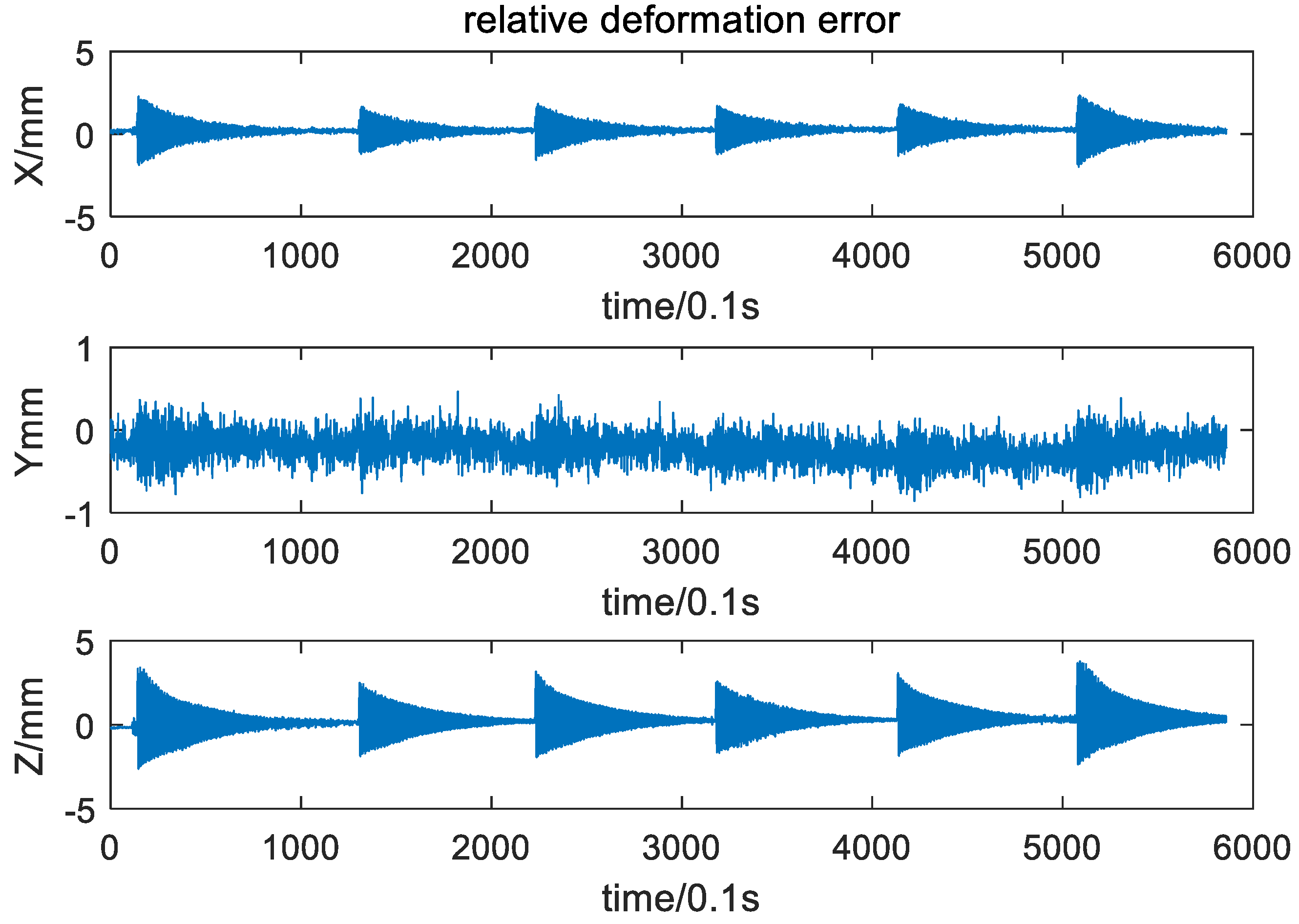
4.2.2. Dynamic Test
5. Conclusions
Author Contributions
Funding
Institutional Review Board Statement
Informed Consent Statement
Data Availability Statement
Conflicts of Interest
References
- Zhu, Z.S.; Tan, H.; Jia, Y.; Xu, Q.F. Research on the Gravity Disturbance Compensation Terminal for High-Precision Position and Orientation System. Sensors 2020, 20, 4932. [Google Scholar] [CrossRef]
- Rigling, B.D.; Moses, R.L. Motion Measurement Errors and Autofocus in Bistatic SAR. IEEE Trans. Image Process. 2006, 15, 1008–1016. [Google Scholar] [CrossRef]
- Liu, Y.H.; Wang, B.; Ye, W.; Ning, X.L.; Gu, B. Global Estimation Method Based on Spatial–Temporal Kalman Filter for DPOS. IEEE Sens. J. 2021, 21, 3748–3756. [Google Scholar] [CrossRef]
- Wang, J.; Liang, X.D.; Ding, C.B.; Chen, L.Y.; Wang, Z.Q.; Li, K. A novel scheme for ambiguous energy suppression in MIMO-SAR systems. IEEE Geosci. Remote Sens. Lett. 2015, 12, 344–348. [Google Scholar] [CrossRef]
- Lu, Z.X.; Li, J.L.; Fang, J.C.; Wang, S.C.; Zhou, S.Y. Adaptive Unscented Two-Filter Smoother Applied to Transfer Alignment for ADPOS. IEEE Sens. J. 2018, 18, 3410–3418. [Google Scholar] [CrossRef]
- Lu, Z.X.; Fang, J.C.; Liu, H.J.; Gong, X.L.; Wang, S.C. Dual-filter transfer alignment for airborne distributed POS based on PVAM. Aerosp. Sci. Technol. 2017, 71, 136–146. [Google Scholar] [CrossRef]
- Gong, X.L.; Chen, L.J.; Fang, J.C.; Liu, G. A transfer alignment method for airborne distributed POS with three-dimensional aircraft flexure angles. Sci. China Inf. Sci. 2018, 61, 190–204. [Google Scholar] [CrossRef] [Green Version]
- Fang, J.C.; Zang, Z.; Gong, X.L. Model and simulation of transfer alignment for distributed POS. J. Chin. Inert. Techn. 2012, 20, 379–385. [Google Scholar]
- Peng, J.Q.; Xu, W.F.; Liang, B. Pose Measurement and Motion Estimation of Space Non-cooperative Targets based on Laser Radar and Stereo-vision Fusion. IEEE Sens. J. 2019, 19, 3008–3019. [Google Scholar] [CrossRef]
- Gadwe, A.; Ren, H. Real-Time 6DOF Pose Estimation of Endoscopic Instruments Using Printable Markers. IEEE Sens. J. 2019, 19, 2338–2346. [Google Scholar] [CrossRef]
- Guo, J.; Zhu, C.A.; Lu, S.L.; Zhang, D.S.; Zhang, C.Y. Vision-based measurement for rotational speed by improving Lucas-Kanade template tracking algorithm. Appl. Opt. 2016, 55, 7186–7194. [Google Scholar] [CrossRef] [PubMed]
- Jiang, F.F.; Zhou, Y.H.; Ling, T.Y.; Zhang, Y.B.; Zhu, Z.Y. Recent Research for Unobtrusive Atrial Fibrillation Detection Methods Based on Cardiac Dynamics Signals: A Survey. Sensors 2021, 21, 3814. [Google Scholar] [CrossRef]
- Burner, A.W.; Liu, T. Videogrammetr Model Deformation Measurement Technique. J. Aircr. 2001, 38, 745–754. [Google Scholar] [CrossRef] [Green Version]
- Liu, Z.; Zhang, G.J.; Wei, Z.Z. Global Calibration of Multi-sensors Vision System Based on Two Planar Targets. J. Mech. Eng. 2009, 45, 228–232. [Google Scholar] [CrossRef]
- Pavlovcic, U.; Arko, P.; Jezersek, M. Simultaneous Hand-Eye and Intrinsic Calibration of a Laser Profilometer Mounted on a Robot Arm. Sensors 2021, 21, 1037. [Google Scholar] [CrossRef]
- Wang, G.; Shang, Y.; Guan, B.L. Flexible Calibration of Setting Relation of a Multi-camera Rig for Non-Overlapping Views. Chin. J. Laser. 2017, 2017, 207–213. [Google Scholar]
- Xu, D.; Tan, M.; Li, Y. Visual Measurement and Control for Robots, 2nd ed.; National Defense Industry Press: Beijing, China, 2010; pp. 132–138. [Google Scholar]
- Wang, P.; Xu, G.L.; Cheng, Y.H.; Yu, Q.D. A Simple, Robust and Fast Method for the Perspective-n-Point Problem. Pattern Recognit. Lett. 2018, 108, 31–37. [Google Scholar] [CrossRef]
- Hartley, R.; Zisserman, A. Multiple View Geometry in Computer Vision, 2nd ed.; Cambridge University Press: Cambridge, UK, 2004; pp. 325–340. [Google Scholar]
- Tsai, R.Y.; Lenz, R.K. A new technique for fully autonomous and efficient 3D robotics hand/eye calibration. IEEE Trans. Robot. Autom. 1989, 5, 345–358. [Google Scholar] [CrossRef] [Green Version]
- Zhang, Z.Y. A Flexible New Technique for Camera Calibration. IEEE Trans. Pattern Anal. Mach. Intell. 2002, 22, 1330–1334. [Google Scholar] [CrossRef] [Green Version]
- Camera Calibration Toolbox for Matlab. Available online: http://www.vision.caltech.edu/bouguetj/calib_doc/ (accessed on 14 October 2015).
- Ding, J.Y.; Pan, Z.K. The Lie group Euler methods of multibody system dynamics with holonomic constraints. Adv. Mech. Eng. 2018, 10, 1–10. [Google Scholar] [CrossRef]
- Park, F.C.; Martin, B.J. Robot sensor calibration: Solving AX = XB on the Euclidean group. IEEE Trans. Robot. Autom. 2002, 10, 717–721. [Google Scholar] [CrossRef]


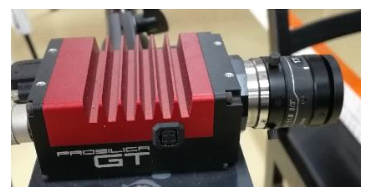
| Camera Parameters | Index |
|---|---|
| Image resolution | 2448 * 2050 |
| Frame rate | 15 fps |
| Focal length | 25 mm |
| Size of CCD pixel | 3.45 μm * 3.45 μm |
| lens | Computar M2518-MPW2 |
| Loads | x-axis | y-axis | z-axis | Baseline | ||Baseline Error|| | ||||
|---|---|---|---|---|---|---|---|---|---|
| Proposed Method | Benchmark | Proposed Method | Benchmark | Proposed Method | Benchmark | Proposed Method | Benchmark | ||
| 1 kg | 556.875 | 556.575 | 6.103 | 7.756 | 10.037 | 10.234 | 556.999 | 556.723 | 0.276 |
| 2 kg | 558.319 | 558.43 | 12.605 | 12.878 | 10.366 | 10.42 | 558.558 | 558.676 | 0.118 |
| 3 kg | 558.916 | 559.112 | 18.043 | 18.007 | 10.832 | 11.231 | 559.312 | 559.515 | 0.203 |
| 4 kg | 559.105 | 559.332 | 25.076 | 25.865 | 11.121 | 11.442 | 559.778 | 560.047 | 0.269 |
| 5 kg | 559.652 | 559.452 | 31.184 | 31.947 | 11.348 | 11.567 | 560.635 | 560.483 | 0.152 |
| 6 kg | 559.863 | 559.763 | 37.219 | 35.743 | 11.602 | 12.012 | 561.219 | 561.032 | 0.187 |
| 7 kg | 560.479 | 560.7 | 43.292 | 43.931 | 11.731 | 12.321 | 562.271 | 562.553 | 0.282 |
| 8 kg | 561.516 | 561.23 | 49.619 | 49.419 | 11.894 | 12.305 | 563.83 | 563.536 | 0.294 |
| Time Periods | x-axis | y-axis | z-axis | Baseline Error |
|---|---|---|---|---|
| 0–100 s | 0.57 | 0.25 | 0.86 | 0.61 |
| 101–200 s | 0.43 | 0.23 | 0.66 | 0.45 |
| 201–300 s | 0.48 | 0.25 | 0.76 | 0.51 |
| 301–400 s | 0.46 | 0.30 | 0.70 | 0.45 |
| 401–500 s | 0.49 | 0.35 | 0.74 | 0.51 |
| 501–586 s | 0.64 | 0.28 | 1.01 | 0.67 |
Publisher’s Note: MDPI stays neutral with regard to jurisdictional claims in published maps and institutional affiliations. |
© 2021 by the authors. Licensee MDPI, Basel, Switzerland. This article is an open access article distributed under the terms and conditions of the Creative Commons Attribution (CC BY) license (https://creativecommons.org/licenses/by/4.0/).
Share and Cite
Liu, Y.; Ye, W.; Wang, B. A Flexible Baseline Measuring System Based on Optics for Airborne DPOS. Sensors 2021, 21, 5333. https://doi.org/10.3390/s21165333
Liu Y, Ye W, Wang B. A Flexible Baseline Measuring System Based on Optics for Airborne DPOS. Sensors. 2021; 21(16):5333. https://doi.org/10.3390/s21165333
Chicago/Turabian StyleLiu, Yanhong, Wen Ye, and Bo Wang. 2021. "A Flexible Baseline Measuring System Based on Optics for Airborne DPOS" Sensors 21, no. 16: 5333. https://doi.org/10.3390/s21165333
APA StyleLiu, Y., Ye, W., & Wang, B. (2021). A Flexible Baseline Measuring System Based on Optics for Airborne DPOS. Sensors, 21(16), 5333. https://doi.org/10.3390/s21165333