Abstract
Echo signals in different regions in the k-space of magnetic resonance imaging (MRI) data possess different amplitudes. The signal-to-noise ratio (SNR) of a received signal can be improved by differentially setting the receiving gain (RG) parameter in different areas of the k-space. Previously, the k-space data splicing method and the gain normalization implementation method were not specifically investigated; however, this study focuses on this aspect. Specifically, to improve the SNR, three RGs and MRI scans are herein designed for each gain parameter using the gradient echo sequence to obtain one group of k-space data. Subsequently, the three groups of experimental k-space data obtained using MRI scans are spliced into one group of k-space data. For the splicing process, a method for gain and phase correction and compensation is developed that normalizes different RG parameters in the k-space. The experimental results indicate that the developed methods improve the SNR by 5–13%. When the RGs are set to other combinations, the k-space data splicing and gain normalization methods presented in this paper are still applicable.
1. Introduction
Signal acquisition research has thus far focused on the maximum signal-to-noise ratio (SNR) at individual amplitude points to prevent saturation under a fixed receiving gain (RG). Several researchers have attempted to improve the SNR by reducing the receiver noise [1,2,3,4,5,6,7,8]. When compared with analog receivers, digital receivers can reduce the noise of nuclear magnetic resonance (NMR) and magnetic resonance imaging (MRI), thereby improving the SNR [1,2,3,4]. For conventional MRI digital receivers (3T), analog-to-digital convertors (ADCs) with a conversion rate of 100 MHz are typically used for under-sampling and analog-to-digital signal conversion [5]. Under the normal temperature operating mode, the SNR of a system does not improve even if the ADC sampling rate exceeds 100 MHz, owing to the impact of physiological noise from the human body [6]. Masoud et al. proposed a 20 GHz superconducting ADC to sample the MRI signals in an ultra-low-temperature environment and reduce the impact of human physiological noise, thereby improving the SNR [6]. However, their proposed superconducting ADC requires ultra-low temperatures to function, which limits its practical application in MRI. Diu and A.T. used redundant information detection to achieve a lower sampling noise and a higher sampling resolution for the internal design of an ADC, further improving the quantization SNR [7,8]. However, because this method involves chip design, its implementation is more complex. In addition to the sampling rate of the ADC being increased, the SNR of the sampling signal can also be improved by increasing the number of bits of the ADC. However, this requires redesigning the spectrometer hardware itself. Therefore, this approach will yield expensive and complex commercial MR systems [9,10].
Because the amplitude of the free induction decay (FID) signal of NMR fluctuates greatly in terms of duration, the method for reducing the receiver noise under a fixed RG proposed in the literature [1,2,3,4,5,6,7,8] leverages the entire resolution of an ADC for the part with a larger amplitude in the signal; however, it does not consider the dynamic range of the signal across the entire period during the quantization process. Although measures have been taken to reduce the sampling noise, the parts of the signal with smaller amplitudes still cannot leverage the full resolution of an ADC [1,2,3,4,5,6,7,8,11], meaning that the maximum possible SNR cannot be achieved. In 2011, Takeda et al. proposed a solution, namely, Apodization after Receiver Gain Increment during Ongoing Sequence with Time (APRICOT). By means of dynamically adjusting the RG, the solution not only increases the SNR of the part with a larger amplitude in the FID signal, but also the receiver gain of the part with a smaller amplitude. Therefore, the small peak signal masked by digital noise can be identified [12]. However, for best results, a series of parameters, including the preamplifier noise index, signal accumulation number, and signal spectrum width, must be matched simultaneously because APRICOT employs an open-loop RG control pattern. Therefore, it is difficult to accurately control the RG via this method. Inspired by the propositions of Takeda et al., Jouda et al. proposed an improved closed-loop RG adjustment method. By monitoring the signal amplitude in real time and adjusting the RG during signal acquisition, they accurately recovered the quantized signals of an ADC. Their method improved the SNR of the FID over the entire period via dynamic adjustment of the RG. However, it requires an accurate closed-loop RG control circuit, which complicates the circuit design [11].
Each NMR scan can only obtain one line of FID data; conversely, with MRI scanning, a group of k-space data can be obtained, in which the k-space contains multiple phase-encoded line data. In turn, each phase-encoded line represents an echo signal. In the echo signal of the same phase-encoded line in the k-space, the amplitude of a low-frequency signal is larger than that of a high-frequency signal. Setting a fixed RG according to the point with the largest amplitude in the echo will not allow the dynamic range of the whole period echo signal to reach the optimum [11,13,14,15]. Kose et al. [13] used the nonlinear RG method utilized in a simulation to compress the low-frequency component of an echo signal and expand the high-frequency component, which greatly improved the SNR. Based on this simulation, Siemens proposed a nonlinear RG scheme [14] and used it to design a type of signal amplitude compression expander, which was installed in the front-end of the ADC device in an MRI receiver. However, this scheme needs to not only meet the dynamic range and compression requirements, but also consider the nonlinear compression signal recoverability, voltage offset, temperature stability, and other factors. Therefore, its implementation poses great challenges to engineers.
Otake et al. [15] proposed a method to improve the SNR of MRI through parallel acquisition. In their scheme, two acquisition circuits were designed to detect the coil induction signal in parallel, one of which was a high-RG acquisition circuit, whereas the other was a low one. The former could ensure that the part of the echo signal with a smaller amplitude reached a larger dynamic range, while the latter could prevent saturation of the part of the echo signal with a larger amplitude. Through analysis, they demonstrated the easy implementation of the method and its ability to improve the SNR of an MRI signal by approximately 6 dB. However, the method needed two acquisition circuits to acquire the coil induction signal of each channel in parallel, which increased the material cost and system complexity of the MRI receiver. Otake et al. [15] also proposed using a histogram to count the high and low gain and phase differences but did not specify the data sample selection method. In recent years, significant progress has been made in improving image SNR through MR image post-processing algorithms [16,17,18]. If the research focus is shifted from image reconstruction to signal-receiving hardware, optimizing the control parameters of the receiving hardware would also be a good option to improve the SNR of the sampled signal.
References [13,14,15] only considered methods to improve the dynamic range of a single echo signal in the k-space. However, among all the phase-encoding lines in the MRI k-space, each line has a distinct echo-signal amplitude. Larger phase-encoding lines have smaller signal amplitudes than those of smaller phase-encoding lines. Therefore, in the process of gain setting, the dynamic range of the entire echo signal cannot be optimized by setting a fixed RG based on the premise that the maximum echo amplitude of all phase-encoding lines in the whole k-space does not saturate [11]. Elliot et al. and Oh et al. found that optimizing the RG parameters of different regions in the MRI k-space without changing the MRI receiver circuit could also increase the dynamic range of the signal [19,20]. Elliot et al. set six RG parameters, with each one set in increments of 6 dB. The sequence was scanned once under every RG parameter, and a group of k-space data was obtained every time. Thus, six groups of k-space data were spliced into one group of k-space data, and a three-dimensional image was obtained using the Fourier transform. When compared with that of the image reconstructed from k-space data at the lowest gain, the quality of the image reconstructed from spliced k-space data was found to have improved [19]. However, that report only mentioned the need for a correction system that could rectify the differences among different gain parameters and did not elaborate on the correction method.
Oh et al. improved the SNR of an MRI image by optimizing the RG parameters of each phase-encoding line in a k-space [20]. In their method, the maximum M(n) of the echo signal of each phase-encoding line was searched, and the optimal gain of each line was determined, where Sm is the maximum of the entire k-space signal, and n is the line number of the phase-encoding line. Their simulation results showed that the optimal sampling bit-width of an ADC would require at least 19 bits under a fixed receiver gain, but only greater than 15 bits under a variable gain. Thus, they significantly reduced the demand for ADC sampling bit bandwidth. As the MRI platform used by Oh et al. did not support the dynamic change in the RG parameters during sequence operation, they used the ideas of Elliot et al. to design the actual experimental paradigm. They obtained a group of k-space data under each gain parameter setting, and then spliced the k-space data obtained under different RG parameters. They stated that different gain parameters must be normalized to the same RG parameter but did not refer to any specific implementation method.
Given this context, this paper proposes a gain-difference correction method that is applicable when different regions of the k-space are assigned different RG parameters. Simultaneously, based on the experimental data, we detail a method to correct and compensate for the RG parameter in each area of the k-space.
2. Experimental Scheme
To improve the SNR of the received signal, we designed three RGs in this study, and a gradient echo (GRE) sequence scan on each RG parameter was conducted to obtain three groups of k-space data. Then, these three groups were spliced into one group. In the splicing process, data obtained under different k-space gain parameters are normalized by the amplitude under the maximum RG parameter. Herein, we also present the methods to correct and compensate for the gain and phase in the normalization process. An SNR comparison between the images reconstructed from the spliced k-space data and the k-space data obtained under the lowest RG was further performed to verify the effectiveness of the proposed k-space data splicing and gain normalization methods.
A commercial 1.5T MR scanner with 16 parallel receiving channels (Alltech Medical Systems LLC, Chengdu, China) was used to comprehensively verify the effectiveness of the research method proposed in this paper. An 8-channel receiver coil was used to conduct the MRI imaging experiment. Additionally, the effectiveness of the proposed method was also verified based on the imaging SNR enhancement effect of each channel. The receiver coil in the system adopts an 8-channel phased array head coil (crown structure design; the upper and lower parts are inseparable), with the eight units of the head coil being similar in size and shape and evenly distributed. This design helps to improve the SNR and uniformity. The coil dimensions were as follows: length = 340 mm and diameter = 240 mm. To calculate the SNR of MRI images more conveniently, a homogeneous water model with a simple internal structure was used as the imaging sample in this study. Homogeneous phantoms (spherical, 200 mm diameter; composition: water (92%), NaCl (5%), and NiSO4·6(H2O) (3%)) were used as imaging samples.
Algorithm 1 shows the main steps of the experiment designed in this paper. The commercial 1.5T MR scanner software interface used in this study has a menu that allows the user to set the RG. The RG parameter is used to control the gain of the MRI spectrometer receiver. The larger this parameter value is, the greater the magnification of the received signal by the spectrometer receiver will be. The parameters for sequence scanning measurement were set as follows: RG: τ, τ − 6, and τ − 12 dB. The attenuation constants τ = 6 dB and 12 dB were obtained via a programmable digital-step attenuation controller in the receiver. TR: 68 ms, TE: 5.2 ms, NEX = 1, receiving channel numbers = 8, excitation slices = 4, scan matrix: 220 × 440, image view matrix: 220 mm × 220 mm, Flip angle: 70°, dw: 8 µs, thickness: 5.0 mm, slice gap: 1.0 mm. During data acquisition, each time an RG control parameter was adjusted, a sequence scan was performed to obtain a group of the original k-space data (8 × 4 × 220 × 440, floating point data).
| Algorithm 1: System execution procedure. |
| Result: Spliced k-space data with enhanced SNR Input: Init: Start GRE sequence scanning and configure the RG parameters as τ, τ − 6, and τ − 12 dB; Step 1: Obtain 3 sets of k-space data: Kτ obtained under RG = τ, Kτ−6 obtained under RG = τ − 6, Kτ−12 obtained under RG = τ − 12; Step 2: Correct the gain difference and phase difference for Kτ and Kτ−6, Correct the gain difference and phase difference for Kτ−6 and Kτ−12, Calculate the gain difference and phase difference for Kτ and Kτ−12; Step 3: Extract Kτ1, Kτ−62, and Kτ−123 from Kτ, Kτ−6, and Kτ−12, respectively to obtain a set of spliced k-space data. Step 4: Compensate for the gain difference between Kτ1, Kτ−62, and Kτ−123; Step 5: Obtain image data by Fourier transform of the spliced k-space data. Output: SNR of the image obtained by Fourier transform of the spliced k-space data |
The k-space data (1 × 1 × 220 × 440) with the first channel and the first slice were extracted to obtain three groups of memory-filling matrix data, Kτ, Kτ–6, and Kτ–12, with RGs of τ, τ − 6, and τ − 12 dB, respectively. The RG corresponds to the amplification factor of the received k-space echo signal in the MR system. Theoretically, the RG differences corresponding to Kτ and Kτ−6 are τ dB − (τ − 6 dB) = 6 dB, i.e., the difference between the amplification factors was 10(6/20) ≈ 2 times, and the difference between the RGs corresponding to Kτ and Kτ–12 was τ dB − (τ − 12 dB) = 12 dB, i.e., the difference between the amplification factors is 10(12/20) ≈ 4 times. A data space of a spliced image was constructed by analyzing the gain and phase differences of the three datasets. Thus, an image could be obtained through the Fourier transform of the spliced data space. Figure 1 illustrates the execution process of the system.
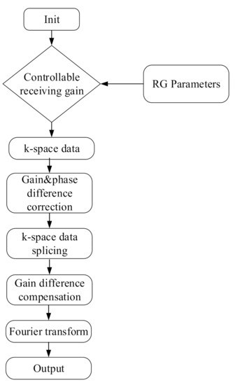
Figure 1.
System execution flowchart.
3. Experimental Verification
The phase-encoding line number filling the memory space of the k-space was denoted by m. To describe the three RG expressions simultaneously in the same image, Kτ was first divided into three areas, namely Kτ1, Kτ2, and Kτ3, respectively, where Kτ1 is m = 1–36, m = 185–220; Kτ2 is m = 37–72, m = 149–184; and Kτ3 is m = 73–148. Similarly, Kτ−6 and Kτ−12 were also divided into three areas. To normalize the data of the three areas to the same RG level, their gain and phase differences must be corrected.
3.1. Data Splicing
Under the same RG in all the areas in the k-space, the amplitude of the echo signal meets the following criteria.
K()1 < K()2 < K()3
Assuming K is the spliced data space, we considered Kτ1 of Kτ as K1 of K, Kτ−62 of Kτ−6 as K2 of K, Kτ−123 of Kτ−12 as K3 of K. Among them, the echo signal of K1 was obtained under the maximum RG to ensure that the echo signal of the K1 area reached the maximum signal dynamic range; the echo signal of K3 was obtained under the minimum RG to ensure that the echo signal of the K3 area did not overflow (shown in Figure 2).
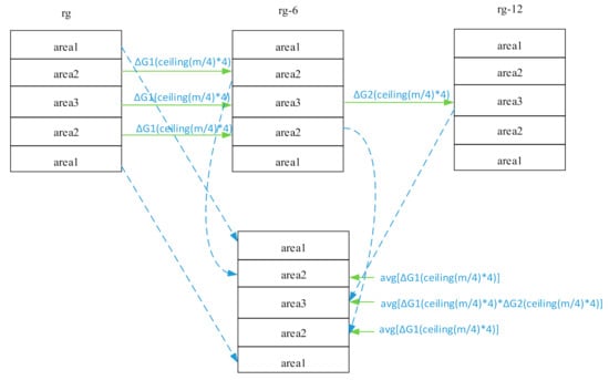
Figure 2.
k-space data splicing and gain correction.
3.2. Gain Difference Correction
In Kτ2 and Kτ3 of Kτ, and Kτ−62 and Kτ−63 of Kτ−6, the same four lines of data were extracted in order every time. The middle N data with the phase-encoding line number ceil(m/4) × 4 were defined as , ; where and are absolute values. The extraction order is as follows:
, the gain difference factor of the corresponding phase-encoding lines of Kτ and Kτ−6, was . In Kτ2 and Kτ3 of Kτ, and Kτ−62 and Kτ−63 of Kτ−6, the sum ΔG1(ceil(m/4) × 4) of all lines and their average value were used to obtain avg[ΔG1(ceil(m/4) × 4)]. The gain difference factor in Kτ2 and Kτ3 of Kτ and Kτ−62 and Kτ−63 of Kτ−6 was avg[ΔG1(ceil(m/4) × 4)].
In Kτ−63 of Kτ−6 and Kτ−123 of Kτ−12, the same four lines of data were extracted in order each time, and the middle N data with the phase-encoding line number ceil(m/4) × 4 were defined as , , ; where and are absolute values. The extraction order is as follows:
, the gain difference factor of the corresponding phase-encoding lines of Kτ−63 and Kτ−123, was . Assuming to be the gain difference factor of the corresponding phase-encoding lines in Kτ3 and Kτ−123, we derive
In Kτ3 and Kτ−123, of all lines were summed and then averaged to obtain , which was the final gain difference factor in Kτ3 and Kτ−123.
According to this method, the gain difference factors of Kτ (Kτ2 and Kτ3) and Kτ−6 (Kτ−62 and Kτ−63) and Kτ3 and Kτ−123 were 2.1173 and 3.9736, respectively.
In Figure 3, the black curve represents the amplitude ratios of Kτ and Kτ−6, and the blue curve represents those of Kτ and Kτ−12. The signal amplitudes of lines 37 to 184 of Kτ, Kτ−6, and Kτ−12 are all distributed above the noise plane. Therefore, in this region, the amplitude ratios are all approximately equal to their theoretical values (2 and 4, respectively).
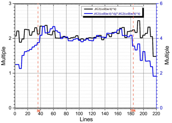
Figure 3.
Gain difference factor calculation.
Most of the effective components of the echo signals in lines 1–36 and 185–220 of Kτ−6 and Kτ−12 were distributed below the noise plane. Because the amplitude was mainly determined by the noise amplitude, the amplitude ratios of Kτ−6 and Kτ−12 in this area tends to one. As the line number moves to the middle region, the echo-signal amplitude gradually rises above the noise plane, and its amplitude ratio approaches two. The echo amplitudes of lines 1–36 and 185–220 of Kτ and Kτ−6 were above the noise plane, and their amplitude ratios were approximately two. The blue curve values corresponding to lines 1–36 and 185–220 were composed of the amplitude ratios of Kτ−6 and Kτ−12, multiplied by those of Kτ and Kτ−6. As the line number migrated to the middle region, the blue curve’s value gradually approached four.
3.3. Gain Compensation
Assuming that the spliced data space is K, we took Kτ1 of Kτ as K1 of K, and Kτ−62 of Kτ−6 as K2 of K. We obtained K2* by multiplying the data amplitude of each line of K2 by ]. We took Kτ−123 of Kτ−12 as K3 of K and obtained K3* by multiplying the data amplitude of each line of K3 by ]. Then, the k-space comprising K1, K2*, and K3* is the compensated k-space.
3.4. Phase Correction
Figure 4 illustrates the k-space signal amplitude distribution with a total of 220 phase-encoding lines and 440 frequency-encoding steps. The k-space central area data have a higher amplitude value, which describes the general contour information of the corresponding homogeneous water model image. The surrounding area data have a lower amplitude value, which describes the detailed information of the corresponding homogeneous water model image. On the one hand, the central area has a higher signal amplitude value than the surrounding region and is less affected by noise. Therefore, the phase difference of the corresponding position signal in the central area tends to be stable. On the other hand, the area surrounding the k-space has a low signal amplitude value and is more affected by noise. This would cause the phase difference of the signals from the surrounding area to considerably fluctuate. When analyzing the phase difference, we considered the middle N steps of each phase-encoding line for the analysis. In this study, we assumed N = 120.
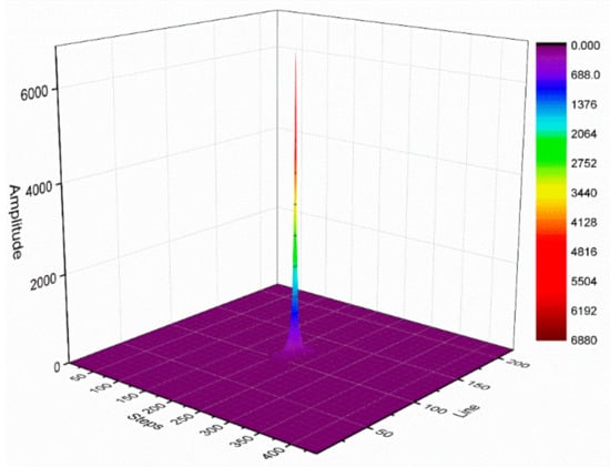
Figure 4.
k-space signal amplitude distribution diagram.
In Kτ2 and Kτ3 of Kτ, and Kτ−62 and Kτ−63 of Kτ−6, we defined the phases of the N steps in the middle of each phase-encoding line as and , where is the number of phase-encoding lines, . The order is as follows:
where . We calculated the distribution of in the k-space, as shown in Figure 5 and Figure 6.
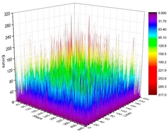
Figure 5.
Three-dimensional statistical diagram of phase difference (error) distributions of Kτ and Kτ−6.
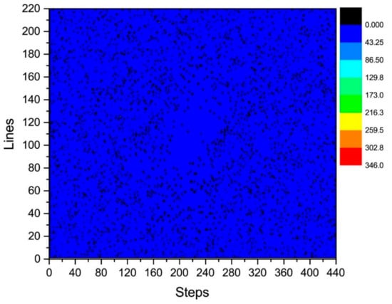
Figure 6.
Statistical diagram of the phase difference (error) of Kτ and Kτ−6.
Figure 5 illustrates the phase difference (error) distributions of the positions of Kτ and Kτ−6 in degrees (°).
Figure 6 illustrates a plane diagram of the statistics of the phase difference (error) between signals at the same positions of Kτ and Kτ−6.
By analyzing the regularities in the phase difference distribution in Figure 4, Figure 5 and Figure 6, we found that the signal amplitude value in the surrounding area of the k-space is low, and the signal is greatly influenced by noise. Therefore, the phase difference of the signal in the area surrounding the k-space fluctuates greatly. The central area has a higher signal amplitude, and the signal is less affected by noise. Therefore, the phase difference of the corresponding position signal in the central area tends to be stable (the phase difference approaches zero). As the signal from the central area is less affected by noise, the phase difference of the corresponding position signal in the area represents the phase difference of the corresponding position signal in the entire k-space. Therefore, the phase differences of all corresponding position signals of Kτ and Kτ−6 were considered to be zero.
In Kτ−63 of Kτ−6 and Kτ−123 of Kτ−12, we defined the phases of the N steps in the middle of each phase-encoding line as and , where is the number of phase-encoding lines, i.e., . Order:
where is the number of phase-encoding lines, i.e., . We then calculated the distribution of in the k-space, as shown in Figure 7 and Figure 8. Figure 7 depicts the phase difference (error) distributions of the corresponding positions of Kτ−6 and Kτ−12 in degrees (°). Figure 8 illustrates the plane diagram of the statistical distribution of phase difference (error) between signals at Kτ−6 and Kτ−12.
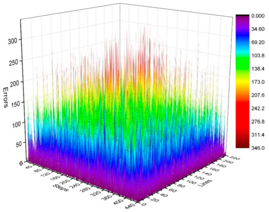
Figure 7.
Three-dimensional diagram of phase difference (error) distributions of Kτ−6 and Kτ−12.
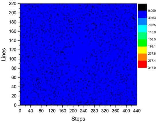
Figure 8.
Statistical graph of phase difference (error) distribution in the plane between Kτ−6 and Kτ−12.
By analyzing the regularities in the distribution of phase difference in Figure 4, Figure 7 and Figure 8, we found that the signal amplitude value in the surrounding area of k-space is low, and the signal is greatly affected by noise; therefore, the phase difference of the signal in the area surrounding the k-space fluctuates strongly. The central area has a higher signal amplitude, and the signal is less affected by noise; therefore, the phase difference of the corresponding position signal in the central area tends to be stable (the phase difference approaches 0). As the signal in the central area is less affected by noise, the phase difference of the corresponding position signal in the central area represents the phase difference of the corresponding position signal in the entire k-space; therefore, the phase differences of all corresponding position signals of Kτ−6 and Kτ−12 were considered to be 0.
The phase difference between Kτ and Kτ−12 was obtained by adding the phase differences between Kτ and Kτ−6 and Kτ−6 and Kτ−12. As observed in Figure 6 and Figure 8, the phase differences between Kτ and Kτ−6 and Kτ−6 and Kτ−12 are zero. Therefore, the phase difference between Kτ and Kτ−12 is also zero.
The spliced k-space data are composed of Kτ1, Kτ−62, and Kτ−123, and these three areas of data are obtained by scanning each GRE sequence under three different RG parameters. Although, in theory, only the receiver hardware has an RG difference during these three scans, the entire physical state of the MRI may not be completely consistent. Therefore, it is necessary to consider whether there is a phase difference between the three areas of the data during the data splicing process.
The controllable RG circuit of the receiver hardware is composed of a fixed amplifier cascaded with a programmable attenuator; hence, by controlling the programmable attenuator, different RGs can be obtained. In addition, when the receiver hardware is set with different RGs, the signal phase may fluctuate randomly at different levels. Therefore, it is necessary to analyze the signal phase difference under different RGs. The phase difference of the corresponding data of Kτ and Kτ−6 is statistically analyzed in Figure 5 and Figure 6. That of the corresponding data of Kτ−6 and Kτ−12 is statistically analyzed in Figure 7 and Figure 8. By calculating the sum of the above two phase differences, the phase difference of Kτ and Kτ−12 is obtained.
3.5. Phase Compensation
After gain compensation, the data phase of K1 remains unchanged. As per the phase correction results, the phase compensation values of both K2* and K3* are defaulted to zero, i.e., the phases of the K2* and K3* data points remain unchanged.
3.6. Experimental Design
A commercial 1.5T MR scanner (Alltech Medical Systems LLC, Chengdu, China) was used to verify the effectiveness of the research method proposed in this paper. In the experiment, an 8-channel head coil was used as the signal induction coil. As each channel was distributed in a different spatial position along the head coil, the maximum sensitivity of each channel was determined according to the spatial distance between the coil channel position and the sample, i.e., the surface of the scanned sample adjacent to the coil channel could produce a higher SNR. As the distance between the scanning sample position and the coil channel increased, the SNR of the signal induced by the coil decreased sharply, resulting in the coil channel being insensitive to the received signals. Each channel of the 8-channel head coil has a different degree of sensitivity in different spatial regions of the scanned sample (homogeneous phantom). This experiment sequentially analyzed the data collected by each channel of the 8-channel head coil and verified the proposed method by contrasting the SNR of the image reconstructed from the k-space data on splicing and the SNR of the reconstructed image from the k-space data obtained at the lowest RG. The area with the highest gray value of the scanned sample was selected as the signal area of the region of interest (ROI), and the four corner background areas of the image area were used as the black area. We used the following SNR calculation formula: SNR = SI/SD, where SI is the average signal intensity of ROI, the St Dev of the four black areas was calculated, respectively, then the total St Dev of the four black areas was calculated, which was averaged to obtain SD.
4. Results
The improvement of the SNR of k-space signals was explored in this study via optimization of the hardware parameters of MRI. At present, this technology is still in the theoretical verification stage, and the equipment is also in the preliminary testing phase. According to the guidelines for medical equipment research, the device does not currently satisfy the conditions to carry out experiments on humans, because it has not yet been assessed for safety; moreover, animal experiments also require further design. To verify the feasibility of the technology, we therefore designed a uniform water model experiment for initial validation. The actual sampling results of the experiment are shown in Figure 6, and the performance comparison is shown in Table 1.

Table 1.
Signal-to-noise ratio (SNR) improvement statistics.
To verify the performance of the proposed method, we produced the SNR maps of 32 of the reconstructed images from the eight channels. We took the first slice from each channel and derived a total of 24 images. In Figure 9, 24 images were the reconstructed images from each channel under different RGs (τ dB, τ − 6 dB and τ − 12 dB), and eight were the images of each channel spliced according to the proposed method. In the experiment, we used the following SNR calculation formula that is commonly used in the field of magnetic resonance: SNR = SI/SD, where SI is the average signal intensity of the phantom area of interest, and SD is the average standard deviation from four corner black areas outside the phantom area. Although the black areas may contain ghost signals that increase the standard deviation, thereby over-estimating the noise, such an error would be the same for all of the images, because this experiment is concerned with a comparison of the measured ratio of signal to noise between test cases rather than the intensity of black noise itself. Therefore, the impact of artifacts on black noise does not affect the relative difference of SNR between multiple groups of comparison trials. Table 1 illustrates the improvement of the SNR between the image reconstructed by splicing the k-space data for each channel and the image reconstructed by the k-space data under the lowest RG.
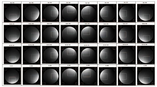
Figure 9.
Eight-channel coil subchannel imaging comparison.
To negate the effect of the difference between the spatial positions of the channel sensitivity, we did not fix the display brightness distribution area on the image. In the analysis, we used the brightest area of the reconstructed image from each channel as the signal area to calculate the changes in the SNR. By comparing the calculation results (Table 1), we found that the SNR of the image reconstructed from the spliced k-space data is significantly higher than that of the image reconstructed from that obtained under the lowest RG (5–13%), demonstrating the effectiveness of the proposed method.
In the actual imaging process of MR equipment, it is necessary to set the Kτ−12 space to the highest RG value possible for the hardware to obtain the best SNR. This will cause the Kτ−6 and Kτ signals to overflow, leading to the non-existence of Kτ−6 and Kτ signals in the actual sampling process. To obtain the effect of the spliced k-space image, two ideal conditions are assumed here, namely that the signals of Kτ−6 and Kτ do not overflow. Kτ−12 is a condition that appears in the actual sampling process. The three spaces of Kτ−12, Kτ−6, and Kτ are spliced to obtain K. Therefore, in the comparative analysis, it is only necessary to compare the data in K with those in Kτ−12 that can be obtained by the actual equipment.
5. Discussion
Table 1 indicates that the SNR difference of the eighth channel in the head coil is relatively small under the RGs of τ − 6 and τ − 12. Therefore, the enhancement of the image SNR corresponding to spliced k-space data of the eighth channel is less evident than that of other channels. This would occur if the actual gain difference between the RGs of τ − 6 and τ − 12 of the eighth channel is smaller than that of the other channels.
References [11,12] discuss the method of improving SNR by adjusting the receiving gain and present an analysis of the SNR improvement effect according to the FID signal of NMR. The method proposed in this paper is mainly intended to improve the image SNR corresponding to k-space data. In reference [13], the effectiveness of the method proposed in this paper was verified by scanning biological structures.
Elliot et al. [19] used water models with structures and teeth to compare the improvement in image detail resolution. Oh et al. [20] used ADC with different resolutions to carry out comparison test. Due to the limitation of current experimental conditions in this paper, we plan to compare our experimental conclusions with those of Elliot’s and Oh’s after we improve our experimental conditions in the next step. Although the quantitative standards of experimental results of previous similar studies are not uniform, they all indicate that the imaging quality was improved. The method proposed in this paper also improves the SNR of MRI images, thus indicating that the proposed gain correction and compensation method is effective. When the RGs are set to other combinations, the k-space data splicing and gain normalization methods presented in this paper are also applicable. In fact, k-space segmentation can also involve more than or less than three areas, but the segmentation into three areas mainly considers the method proposed in this paper through fewer correction and compensation steps.
ADC is a part of the MRI hardware, and ADC quantization noise has a certain impact on image SNR. The main purpose of this paper is to make full use of the ADC resolution through the variable gain in order to improve the SNR of the digital signal after the ADC quantization. When a homogeneous phantom is used for scanning and imaging, the distribution of image black noise is more uniform, and the SNR value can be more accurately calculated using image data. With the same scanning time, a higher SNR results in a higher spatial resolution; if the spatial resolution is the same, the result is a higher temporal resolution. In future work, we will continue to improve the research equipment and use the standard MR resolution phantom for spatial and temporal resolution tests of images.
6. Conclusions
To improve the SNR of the received signal, three RGs were designed in this study, and a GRE sequence scan on each RG parameter was conducted to obtain three groups of k-space data. Then, these three groups were spliced into one group. In the splicing process, data obtained under different k-space gain parameters are normalized by the amplitude under the maximum RG parameter. Herein, we also present the methods to correct and compensate for the gain and phase in the normalization process. An SNR comparison between the images reconstructed from the spliced k-space data and the k-space data obtained under the lowest RG was further performed to verify the effectiveness of the proposed k-space data splicing and gain normalization methods. The experimental results indicate that the developed methods improve the SNR by 5–13%, indicating that the method proposed in this paper is effective.
Author Contributions
Methodology, L.W., S.Z. and T.Z.; formal analysis, L.W., T.Z. and S.Z.; data curation, L.W. and S.Z.; writing—original draft preparation, L.W. and S.Z.; writing—review and editing, L.W., T.Z. and S.Z. All authors have read and agreed to the published version of the manuscript.
Funding
This work was supported by the Sichuan Science and Technology Program under Grant 2019YJ0181; the Sichuan Province Academic and Technical Leader Training Funded Projects under Grant 13XSJS002; the National Key Research and Development Program of China under Grants 2016YFC0100800 and 2016YFC0100802; the Foundation of Ph.D. Scientific Research of Neijiang Normal University under Grant 18B19; the China Postdoctoral Science Foundation funded under Grant 2020M683294; and the Sichuan applied psychology research center of Chengdu Medical College Funded Projects under Grant CSXL-21103.
Institutional Review Board Statement
Not applicable.
Informed Consent Statement
Not applicable.
Data Availability Statement
Not applicable.
Conflicts of Interest
The authors declare no conflict of interest.
References
- Hashimoto, S.; Kose, K.; Haishi, T. Comparison of analog and digital transceiver system for MR imaging. Magn. Reson. Med. Sci. 2014, 13, 285–291. [Google Scholar] [CrossRef] [PubMed]
- Pikulski, M.; Shiroka, T.; Ott, H.-R.; Mesot, J. A firmware-defined digital direct-sampling NMR spectrometer for condensed matter physics. Rev. Sci. Instrum. 2014, 85, 093906. [Google Scholar] [CrossRef] [PubMed]
- Qin, X.; Zhang, W.; Wang, L.; Zhao, Y.; Tong, Y.; Rong, X. An FPGA-based hardware platform for the control of spin-based quantum systems. IEEE Trans. Instrum. Meas. 2020, 69, 1127–1139. [Google Scholar] [CrossRef]
- Doll, A. Pulsed and continuous-wave magnetic resonance spectroscopy using a low-cost software-defined radio. AIP Adv. 2019, 9, 115110. [Google Scholar] [CrossRef]
- Cosmus, T.C.; Parizh, M. Advances in whole-body MRI magnets. IEEE Trans. Appl. Supercond. 2011, 21, 2104–2109. [Google Scholar] [CrossRef]
- Radparvar, M.; Talalaevskii, A.; Webber, R.J.; Kadin, A.M.; Track, E.K.; de Graaf, R.A.; Nixon, T.W.; Rothman, D.L. Superconductor analog-to-digital converter for high-resolution magnetic resonance imaging. IEEE Trans. Appl. Supercond. 2015, 25, 1400505. [Google Scholar] [CrossRef]
- Luu, D.K.; Nguyen, A.T.; Yang, Z. Achieving super-resolution with redundant sensing. IEEE Trans. Biomed. Eng. 2019, 66, 2200–2209. [Google Scholar] [CrossRef] [PubMed]
- Nguyen, A.T.; Xu, J.; Yang, Z. A 14-bit 0.17 mm2 SAR ADC in 0.13 μm CMOS for high precision nerve recording. In Proceedings of the 2015 IEEE Custom Integrated Circuits Conference (CICC), San Jose, CA, USA, 28–30 September 2015; pp. 1–4. [Google Scholar]
- Christodoulou, A.G.; Lingala, S.G. Accelerated dynamic magnetic resonance imaging using learned representations: A new frontier in biomedical imaging. IEEE Signal. Process. Mag. 2020, 37, 83–93. [Google Scholar] [CrossRef]
- He, S.; Jalal, B. Fast super-resolution in MRI images using phase stretch transform, anchored point regression and zero-data learning. In Proceedings of the 2019 IEEE International Conference on Image Processing (ICIP), Taipei, Taiwan, 22–25 September 2019; pp. 2876–2880. [Google Scholar]
- Jouda, M.; Fuhrer, E.; Silva, P.; Korvink, J.G.; MacKinnon, N. Automatic adaptive gain for magnetic resonance sensitivity enhancement. Anal. Chem. 2019, 91, 2376–2383. [Google Scholar] [CrossRef] [PubMed]
- Takeda, K.; Takegoshi, K. Noise reduction by dynamic signal preemphasis. J. Magn. Reson. 2011, 208, 305–308. [Google Scholar] [CrossRef] [PubMed][Green Version]
- Kose, K.; Endoh, K.; Inouye, T. Nonlinear amplitude compression in magnetic resonance imaging: Quantization noise reduction and data memory saving. IEEE AES Mag. 1990, 5, 27–30. [Google Scholar] [CrossRef]
- Bollenbeck, J.; Vester, M.; Oppelt, R.; Kroeckel, H.; Schnell, W. A high performance multi-channel rf receiver for magnet resonance imaging systems. In Proceedings of the International Society for Magnetic Resonance in Medicine, Miami, FL, USA, 7–13 May 2005; p. 13. [Google Scholar]
- Otake, Y.; Kose, K.; Haishi, T. A solution to the dynamic range problem in MRI using a parallel image acquisition. Concepts Mag. Reson. Part B Mag. Reson. Eng. 2006, 29B, 161–167. [Google Scholar] [CrossRef]
- Srivastava, A.; Bhateja, V.; Tiwari, H.; Satapathy, S.C. Restoration algorithm for Gaussian corrupted MRI using non-local averaging. Inf. Syst. Des. Intell. Appl. 2015, 340, 831–840. [Google Scholar]
- Tripathi, P.C.; Bag, S. CNN-DMRI: A convolutional neural network for denoising of magnetic resonance images. Pattern Recognit. Lett. 2020, 135, 57–63. [Google Scholar] [CrossRef]
- Chen, X.-L. Research on Denoising of Brain MRI of Alzheimer’s Disease Based on BM3D Algorithm. Int. J. Health Syst. Transl. Med. IJHSTM 2021, 1, 33–43. [Google Scholar]
- Elliott, M.A.; Insko, E.K.; Greenman, R.L.; Leigh, J.S. Improved resolution and signal-to-noise ratio in MRI via enhanced signal digitization. J. Magn. Reson. 1998, 130, 300–304. [Google Scholar] [CrossRef] [PubMed]
- Oh, C.H.; Ryu, Y.C.; Hyun, J.H.; Bae, S.H.; Chung, S.T.; Park, H.W.; Kim, Y.G. Dynamic range expansion of receiver by using optimized gain adjustment for high-field MRI. Concepts Mag. Reson. Part A Bridg. Educ. Res. 2010, 36, 243–254. [Google Scholar] [CrossRef]


Publisher’s Note: MDPI stays neutral with regard to jurisdictional claims in published maps and institutional affiliations. |
© 2021 by the authors. Licensee MDPI, Basel, Switzerland. This article is an open access article distributed under the terms and conditions of the Creative Commons Attribution (CC BY) license (https://creativecommons.org/licenses/by/4.0/).