
Energy-Efficient Adaptive Sensing Scheduling in Wireless Sensor Networks Using Fibonacci Tree Optimization Algorithm


Abstract
:1. Introduction
- A novel system model of wireless sensor network is introduced;
- An adaptive sensing scheduling strategy based on event occurrence behavior is proposed;
- The scheduling problem is formulated as an optimization problem and is solved by a Fibonacci tree optimization algorithm.
2. Related Work
2.1. Sensing Scheduling Strategies
- Network Structure. The network structure can be flat or hierarchical.
- Sensing Area: The sensing area can be 2-D circular or 3-D spherical.
- Time Synchronization. The sensors are synchronized in time, and can be woken up simultaneously for the next scheduling round.
- Failure Model. Almost all the studies assume that sensors fail when energy is exhausted.
- Sensor Mobility. Most studies have assumed that the sensor is immobile.
- Location Information. These studies typically associate location information with whether, or how much, a sensor’s sensing area overlaps with its neighbor’s.
- Distance Information. The distance information can be inferred from the location information.
- Maximizing Network Lifetime. This is a goal that is hard not to consider.
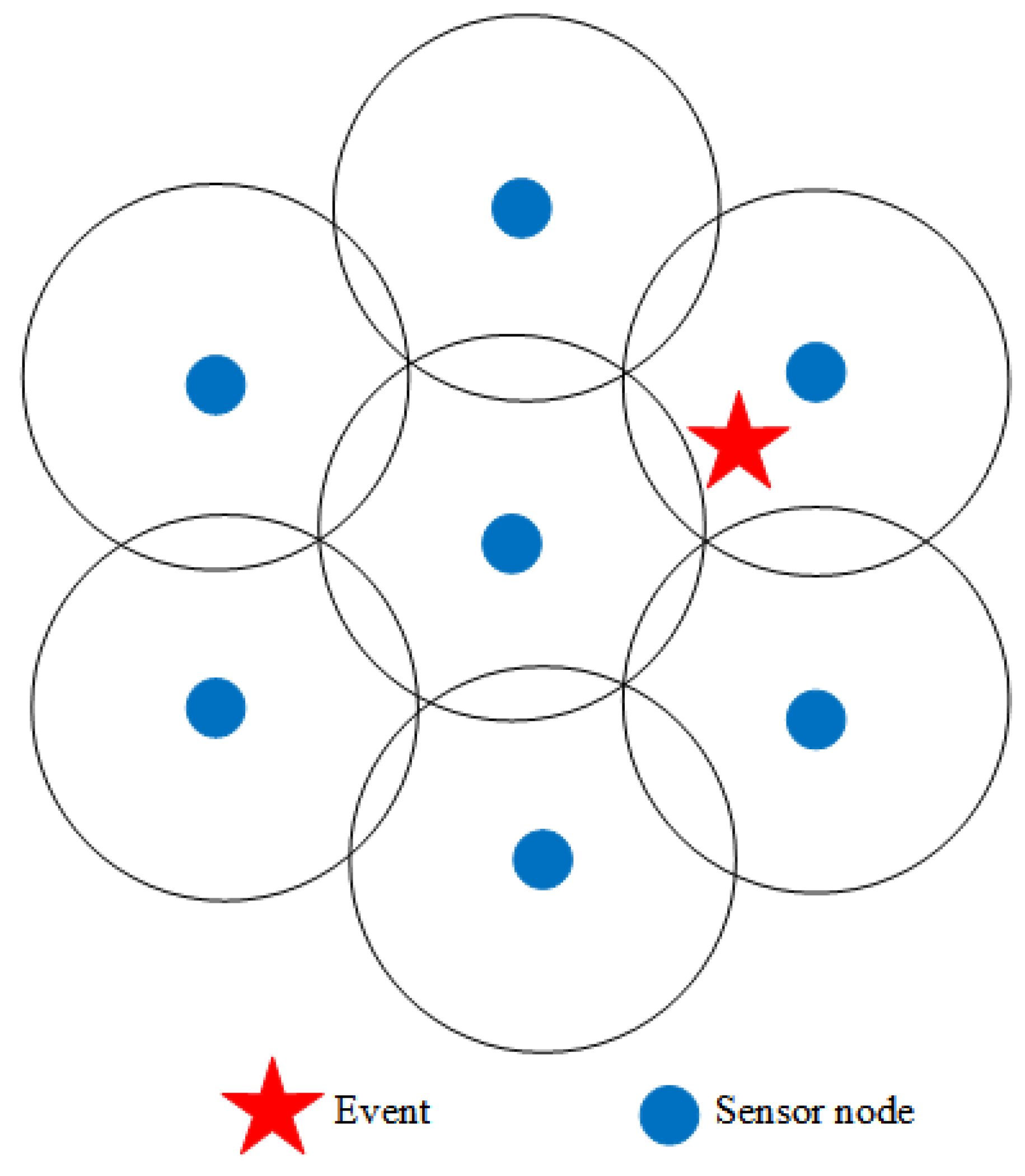
- Sensing Coverage. A network is said to achieve k-coverage if any event occurs within the jurisdiction of at least k sensors. 1-overage is a minimum requirement for WSN.
- Network Connectivity. The developers applaud a model that offers a particular network connectivity needed by the application, but this requires a very high sensor density.
- Balanced Energy Usage. In the case of a sensing coverage breach, when a node runs out of power before others, some studies endeavor to spread the energy utilization evenly among each node.
- Simplicity. Sensors have exceptionally restricted memory space and limited computation power. For this reason, simple schemes are more popular.
- Robustness: Robustness measures how well a network can withstand downtime and crashes.
2.2. Optimization Algorithms for Multi-Modal Function
3. System Model
3.1. Basic Assumptions
- A1: The network structure is flat. All nodes are homogeneous with the same energy budget.
- A2: The positions of sensor nodes are uniformly distributed.
- A3: The sensing area is 2-D.
- A4: The transmission/sensing radii are tunable.
- A5: Time is asynchronous. It is hard to coordinate sensors without a central controller but, otherwise, the central controller incurs a performance penalty. So, sensors embrace asynchronous scheduling—every sensor autonomously decides its duty cycle without synchronizing with each other.
- A6: The sensor node can be movable.
- A7: Location information is unknowable.
- A8: Distance information is unknowable.
3.2. Location Distribution and Sensing Radii
3.3. Event Occurrence and Detection
3.4. Energy Depletion
3.5. Scheduling Model
3.6. Sensing Coverage
3.7. Problem Formulation
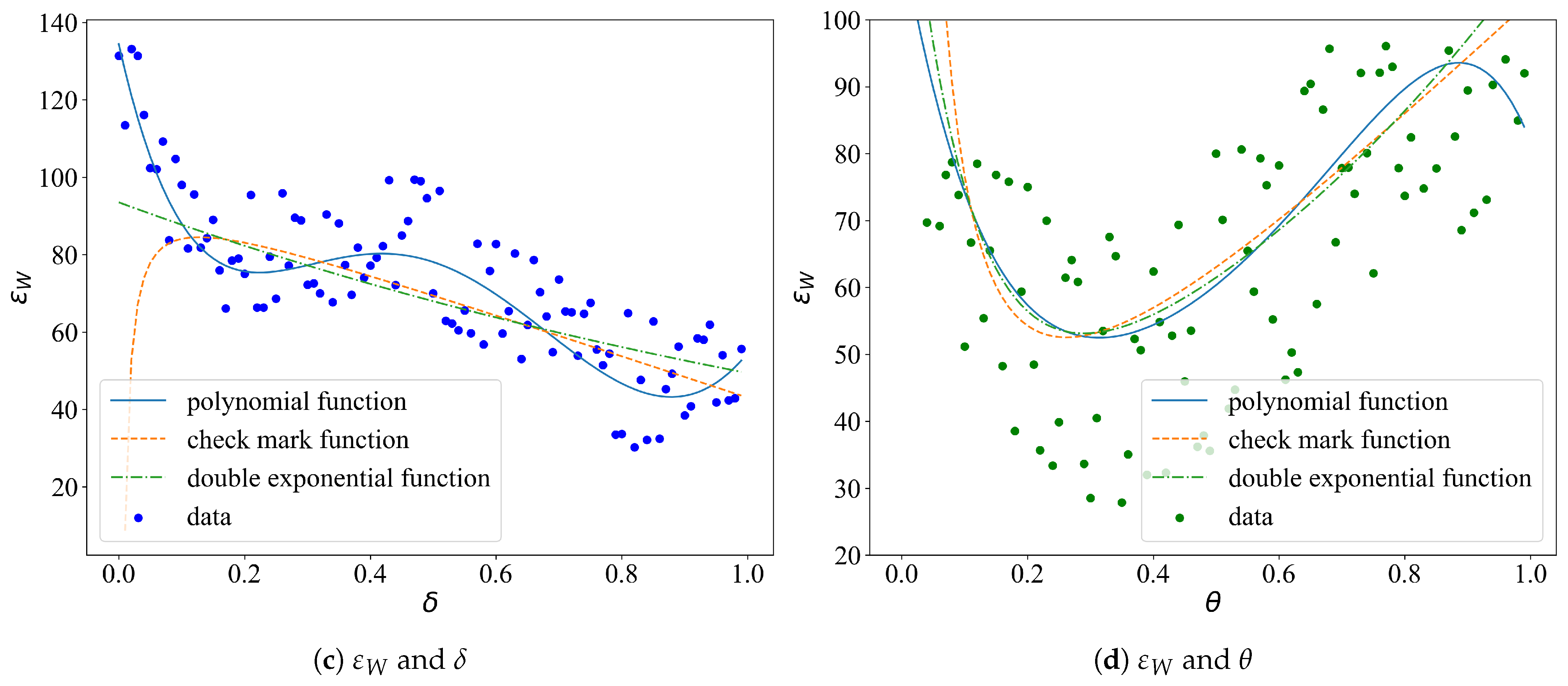
- Presume a functional form. Commonly used function forms include: polynomial function, exponential function, logarithmic function, trigonometric function, and so forth.
- Determine the indeterminate coefficients. Using the least square method, point group center method, random fuzzy method, and so on, to determine the coefficients of the function. Of those, the least square method is the most commonly used.
- Evaluation. The imitative effect can be measured by the mean square error (MSE) or the degree of fit (R2).
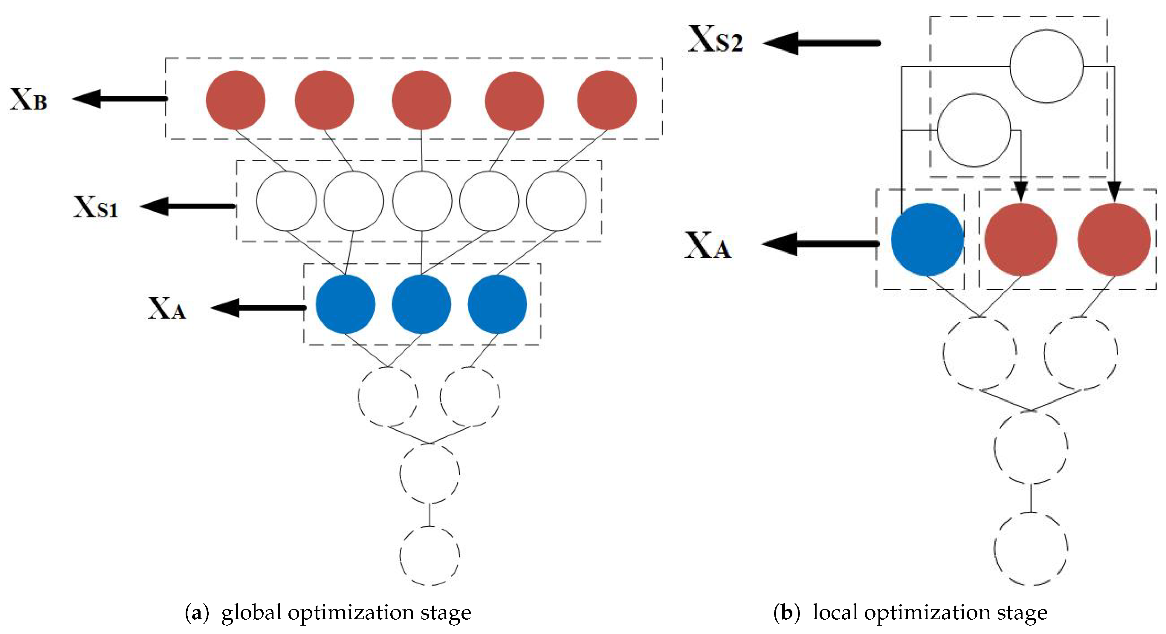
4. Fibonacci Tree Optimization Algorithm
| Algorithm 1: Pseudo-code of Fibonacci branch generation process |
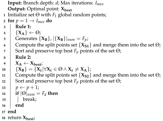 |
5. Analysis
5.1. Why FTO Algorithm Is Chosen for Parameter Optimization?
- In the FTO algorithm, the growth of a Fibonacci tree is based on the optimal points of the latest generation, which is a process of competitive elimination. If there are peaks with different heights, the smaller peaks will be removed in the optimization process. Hence, the global optima can be achieved.
- The inner structure of the FTO algorithm meets the golden ratio all over. With each iteration, the separation of the golden ratio rapidly compresses the search space, providing the local optimal solution. It is adapted to the optimization of multi-modal functions. Conversely, most heuristic algorithms are based on the probabilistic search; they are essentially trial and error methods. It may take thousands or even millions of iterations, which is uneconomical and slow.
- The FTO setup only concerns the initial Fibonacci number, which is exquisite and simple. The typical way to obtain multiple local extremums of the multi-modal function using heuristic algorithms is the niche technology. Setting population parameters has a significant impact on the optimistic effects.
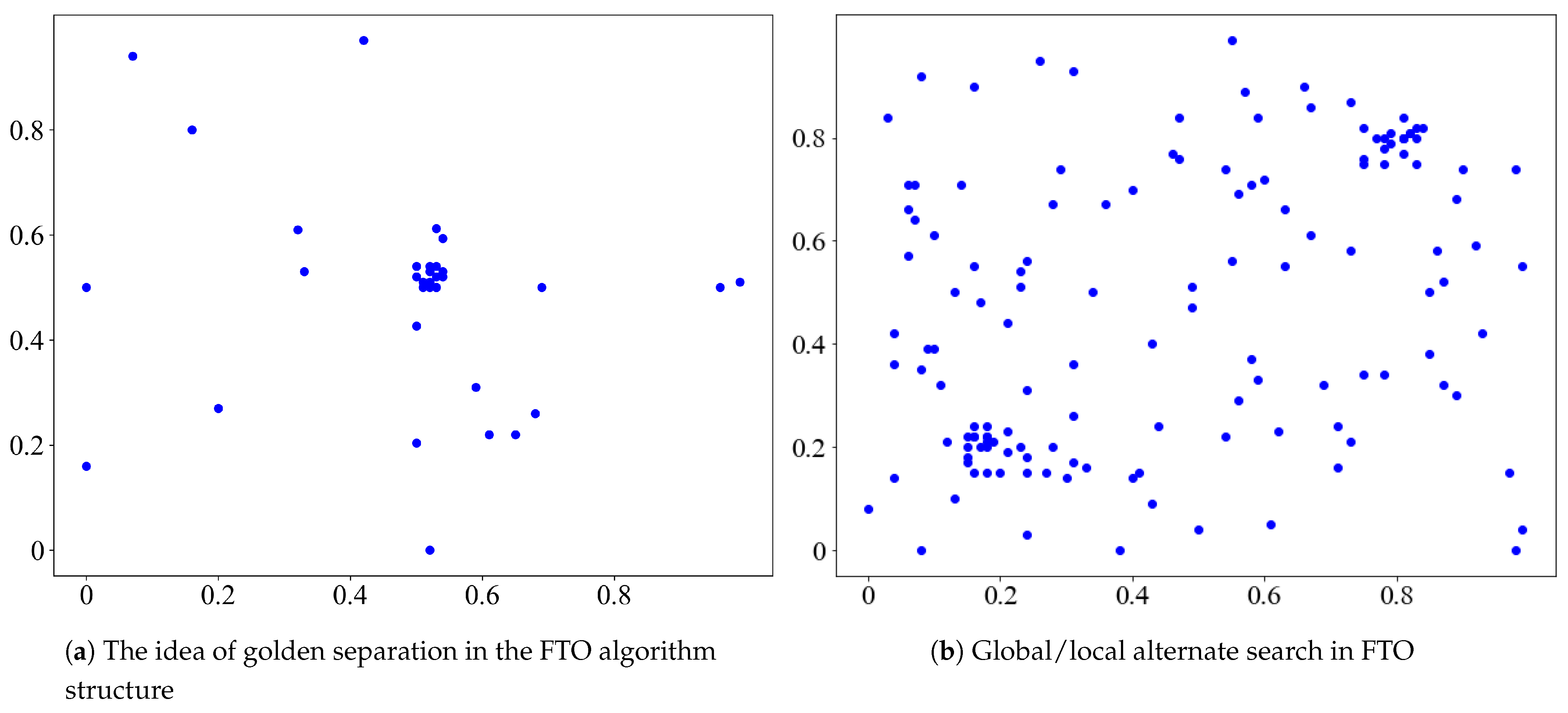
- Just like most heuristic algorithms, FTO is also inspired by natural phenomena—plant phototropism. Plants flourish more in sunny areas. To solve the optimization of the multi-modal function, FTO considers the global search space as a sunlit area. The hit probability is sustained and stable. The lush areas refer to the local search process, reflecting the fact that FTO can alternate between global and local searches.
- It fully utilizes the computer memory to save the optimization process and therefore is traceable.
5.2. Why Do We Claim FTOS Strategy Is Superior to Other Scheduling Strategies?
- Some of the latest scheduling strategies, such as LEACH, work under strict assumptions; for example, the network structure is flat, nodes are densely distributed, time is synchronized, and so forth. The FTOS strategy does not require time synchronization (centralized scheduling); each node independently determines the duty cycle; node density is not important; the location and distance information is not needed.
- The FTOS strategy determines the scheduling parameters as per the occurrence of events from the previous period, which is very scalable.
- Once the parameters are determined, they remain unchanged in the coming hours; you can easily deploy them.
6. Experiment
6.1. Experimental Setup
6.2. Train
6.2.1. Function Fitting
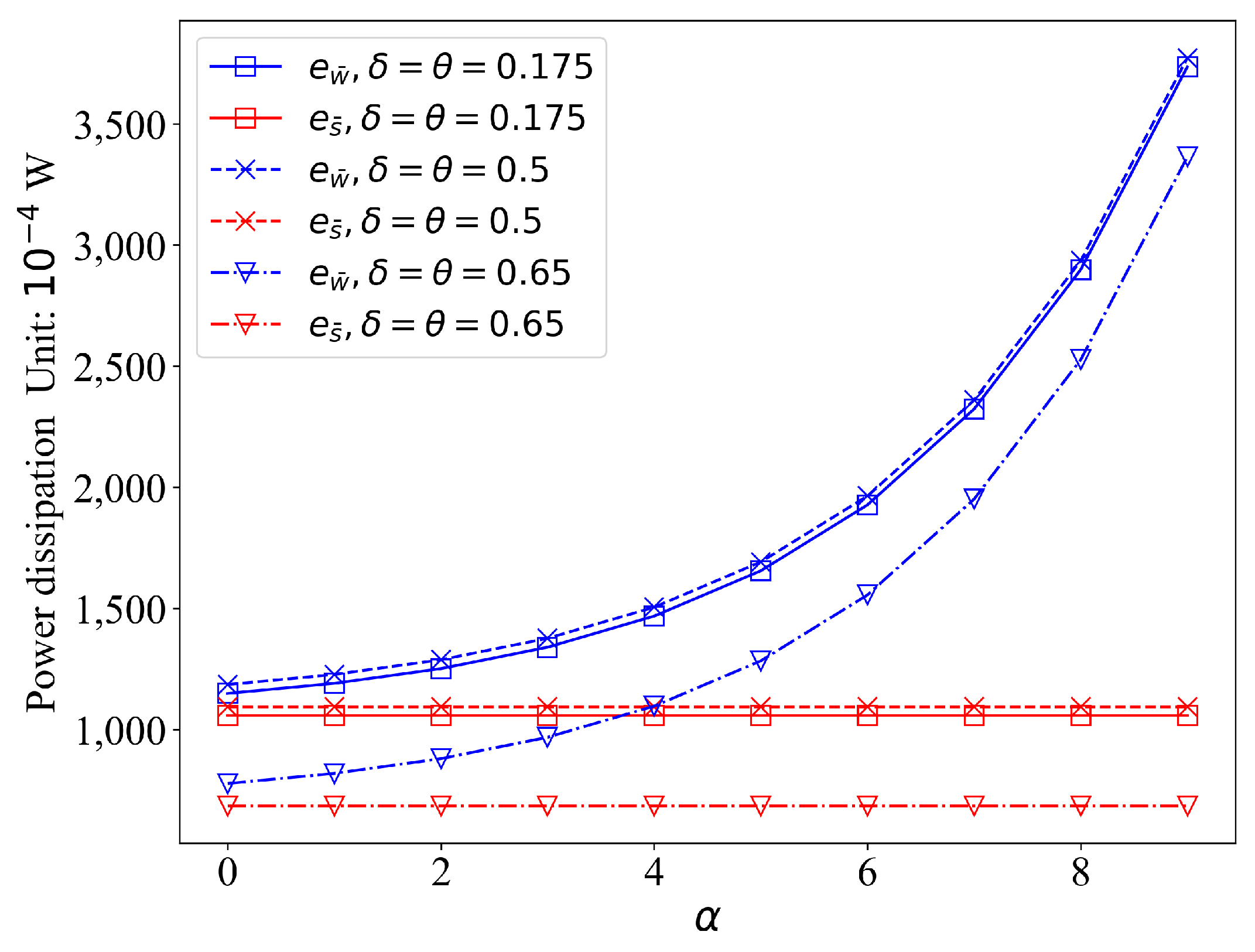
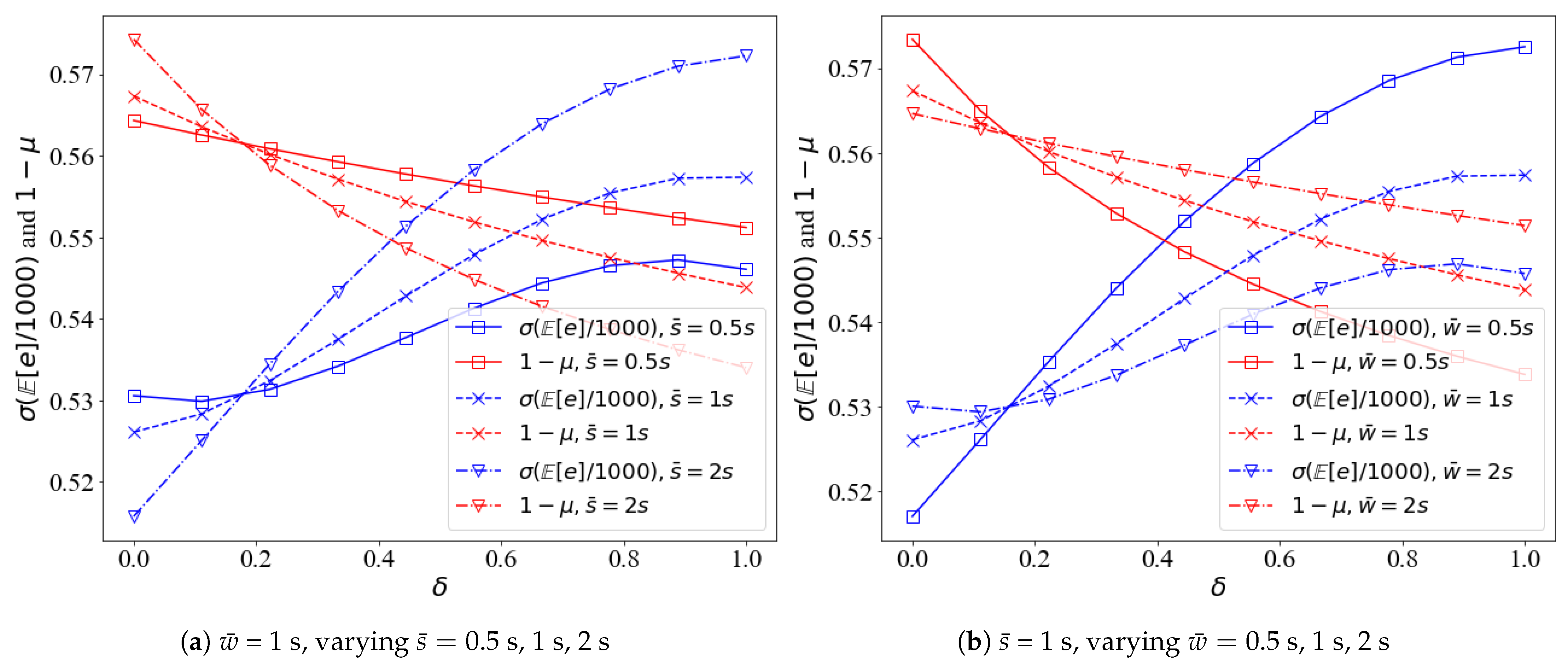
6.2.2. Univariate Analysis
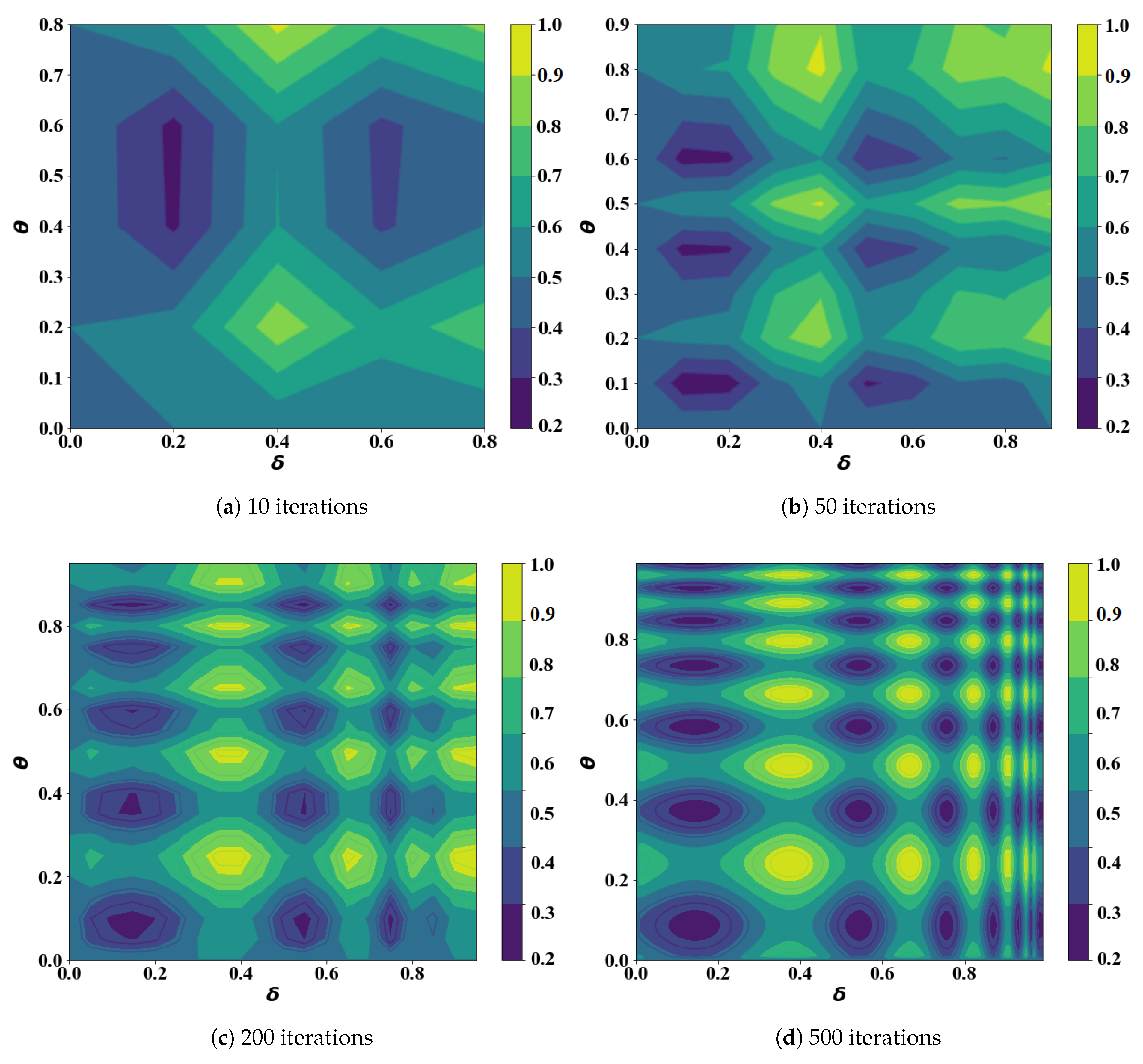
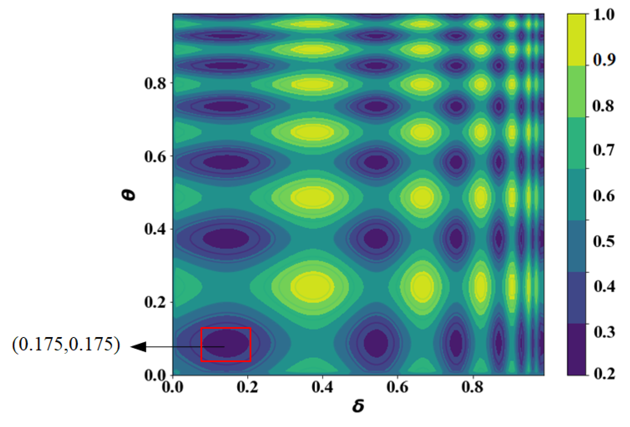
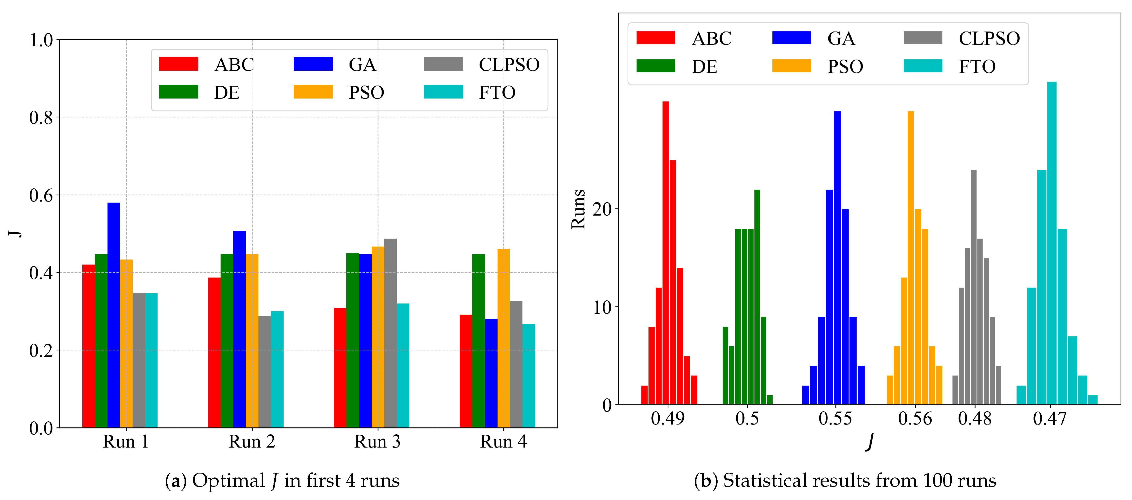
6.2.3. Optimization
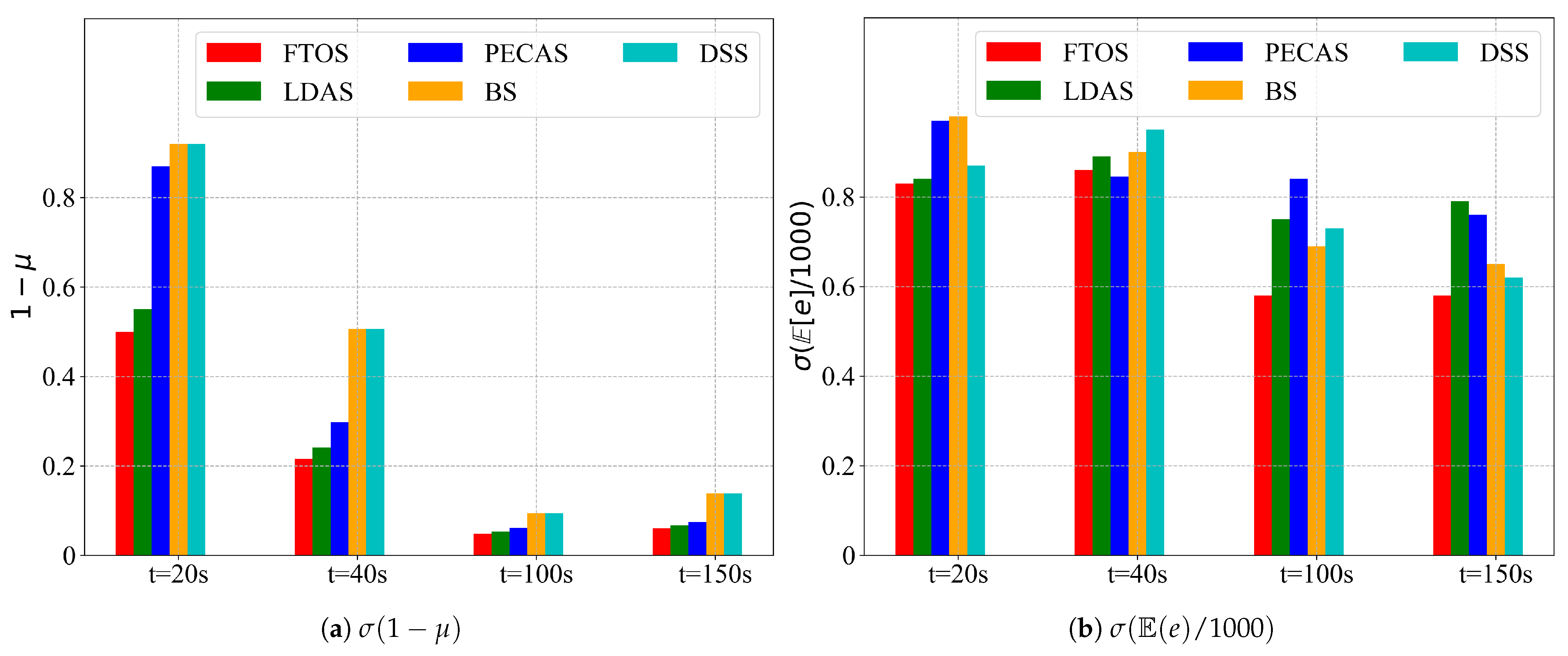
6.3. Test
7. Deficiencies and Unresolved Issues
- Selection of fitting functions. Some simple fitting functions are selected by experience to simulate the relationship between variables related to the objective function and the parameters of the scheduling strategy. The results are indeed good, but other fitting functions are still worth trying.
- Selection of sensors. The diffuse reflection photoelectric infrared proximity sensor, E3F-DS100P1, has a sensing radius of 3~5 m. If you have the budget to pay, you had better use sensors with a larger sensing radius and more accuracy, for example, laser radar.
- Too few nodes. Because of the insufficient number of devices we have, we have only configured a 3-node network. Experiments with more nodes would be more convincing.
8. Conclusions
Author Contributions
Funding
Institutional Review Board Statement
Data Availability Statement
Acknowledgments
Conflicts of Interest
References
- Phan, K.T.; Huynh, P.; Nguyen, D.N.; Ngo, D.T.; Hong, Y.; Le-Ngoc, T. Energy-Efficient Dual-Hop Internet of Things Communications Network with Delay-Outage Constraints. IEEE Trans. Ind. Inform. 2021, 17, 4892–4903. [Google Scholar] [CrossRef]
- Boddu, N.; Boba, V.; Vatambeti, R. A Novel Georouting Potency Based Optimum Spider Monkey Approach for Avoiding Congestion in Energy Efficient Mobile Ad-hoc Network. Wirel. Pers. Commun. 2021. [Google Scholar] [CrossRef]
- Sheng, Z.; Mahapatra, C.; Zhu, C.; Leung, V.C.M. Recent Advances in Industrial Wireless Sensor Networks Toward Efficient Management in IoT. IEEE Access 2015, 3, 622–637. [Google Scholar] [CrossRef]
- Solis, F.; Fernández Bocco, Á.; Galetto, A.C.; Passetti, L.; Hueda, M.R.; Reyes, B.T. A 4GS/s 8-bit time-interleaved SAR ADC with an energy-efficient architecture in 130 nm CMOS. Int. J. Circ. Theory Appl. 2021. [Google Scholar] [CrossRef]
- Li, H.; Wang, Z.; Wang, H. An energy-efficient power allocation scheme for Massive MIMO systems with imperfect CSI. Digit. Signal Process. 2021, 112, 102964. [Google Scholar] [CrossRef]
- Begum, S.; Wang, S.; Krishnamachari, B.; Helmy, A. ELECTION: Energy-efficient and low-latency scheduling technique for wireless sensor networks. In Proceedings of the 29th Annual IEEE Conference on Local Computer Networks (LCN), Tampa, FL, USA, 16–18 November 2004. [Google Scholar]
- Dantu, R.; Abbas, K.; O’Neill, M., II; Mikler, A. Data centric modelling of environmental sensor networks. In Proceedings of the IEEE Globecom, Dallas, TX, USA, 29 November–3 December 2004; pp. 447–452. [Google Scholar]
- Lee, J.; Lee, D.; Kim, J.; Cho, W.; Pajak, J. A dynamic sensing cycle decision scheme for energy efficiency and data reliability in wireless sensor networks. Lect. Notes Comput. Sci. 2007, 4681, 218–229. [Google Scholar]
- Jain, A.; Chang, E.Y. Adaptive sampling for sensor networks. In Proceedings of the International Workshop on Data Management for Sensor Networks, Toronto, ON, Canada, 30 August 2004; Volume 72, pp. 10–16. [Google Scholar]
- Jothiraj, S.; Balu, S.; Rangaraj, N. An efficient adaptive threshold-based dragonfly optimization model for cooperative spectrum sensing in cognitive radio networks. Int. J. Commun. Syst. 2021, 34, e4829. [Google Scholar] [CrossRef]
- Chen, S.; Shao, D.; Shu, X.; Zhang, C.; Wang, J. FCC-Net: A Full-Coverage Collaborative Network for Weakly Supervised Remote Sensing Object Detection. Electronics 2020, 9, 1356. [Google Scholar] [CrossRef]
- Franceschi, S.; Chirici, G.; Fattorini, L.; Giannetti, F.; Corona, P. Model-assisted estimation of forest attributes exploiting remote sensing information to handle spatial under-coverage. Spat. Stat. 2021, 41, 100472. [Google Scholar] [CrossRef]
- He, T. Energy-efficient surveillance system using wireless sensor networks. In Proceedings of the MobiSys 04, Boston, MA, USA, 6–9 June 2004. [Google Scholar]
- Wu, K. Lightweight deployment-aware scheduling for wireless sensor networks. ACM/Kluwer Mob. Netw. Appl. 2005, 10, 837–852. [Google Scholar] [CrossRef] [Green Version]
- Zhang, Y.; Zhang, D.; Vance, N.; Li, Q.; Wang, D. A Light-weight and Quality-aware Online Adaptive Sampling Approach for Streaming Social Sensing in Cloud Computing. In Proceedings of the 24th IEEE International Conference on Parallel and Distributed Systems (ICPADS), Singapore, 11–13 December 2018. [Google Scholar]
- Ye, F.; Zhong, G.S.; Zhang, L. PEAS: A robust energy conserving protocol for long-lived sensor networks. In Proceedings of the IEEE International Conference on Network Protocols (ICNP), Paris, France, 12–15 November 2002. [Google Scholar]
- Liu, C.H.; Zhao, J.; Zhang, H.; Guo, S.; Leung, K.K.; Crowcroft, J. Energy-Efficient Event Detection by Participatory Sensing under Budget Constraints. IEEE Syst. J. 2017, 11, 2490–2501. [Google Scholar] [CrossRef]
- Friderikos, V.; Papadaki, K.; Wisely, D.; Aghvami, H.A. Non-Independent Randomized Rounding for Link Scheduling in Wireless Mesh Networks. In Proceedings of the 64th IEEE Vehicular Technology Conference, Montreal, QC, Canada, 25–28 September 2006. [Google Scholar]
- Sun, M. Adaptive Sensing Schedule for Dynamic Spectrum Sharing in Time-Varying Channel. IEEE Trans. Veh. Technol. 2018, 67, 5520–5524. [Google Scholar] [CrossRef] [Green Version]
- Hanef, M.; Deng, Z. Design challenges and comparative analysis of cluster based routing protocols used in Wireless Sensor Networks for improving network lifetime. Adv. Inf. Sci. Serv. Sci. 2012, 4, 450–459. [Google Scholar]
- Alam, K.M.; Kamruzzaman, J.; Karmakar, G.; Murshed, M. Dynamic adjustment of sensing range for event coverage in wireless sensor networks. J. Netw. Comput. Appl. 2014, 46, 139–153. [Google Scholar] [CrossRef]
- Cichon, K.; Kliks, A.; Bogucka, H. Energy-efficient cooperative spectrum sensing: A survey. IEEE Commun. Surv. Tutor. 2016, 18, 1861–1886. [Google Scholar] [CrossRef]
- Liu, J.L.; Ravishankar, C.V. LEACH-GA: Genetic Algorithm-based energy efficient adaptive clustering protocol for Wireless Sensor Networks. Int. J. Mach. Learn. Comput. 2011, 1, 79–85. [Google Scholar] [CrossRef] [Green Version]
- Salim, A.; Osamy, W.; Khedr, A.M. IBLEACH: Intra-balanced Leach protocol for Wireless Sensor Networks. Wirel. Netw. 2014, 20, 1515–1525. [Google Scholar] [CrossRef]
- Mishra, S.; Yaduvanshi, R.; Dubey, K.; Rajpoot, P. ESS-IBAA: Efficient, short, and secure ID-based authentication algorithm for wireless sensor network. Int. J. Commun. Syst. 2021, 34, e4764. [Google Scholar] [CrossRef]
- Heo, N.; Varshney, P.K. An intelligent deployment and clustering algorithm for adistributed mobile sensor network. In Proceedings of the IEEE International Conference on Systems, Man and Cybernetics, Washington, DC, USA, 5–8 October 2003. [Google Scholar]
- Song, C. Selective CS: An Energy-Efficient Sensing Architecture for Wireless Implantable Neural Decoding. IEEE J. Emerg. Sel. Top. Circuits Syst. 2018, 8, 201–210. [Google Scholar] [CrossRef]
- Sendra, S.; Lloret, J.; Garcia, M.; Toledo, J.F. Power saving and energy optimization techniques for wireless sensor neworks. J. Commun. 2011, 6, 439–459. [Google Scholar] [CrossRef]
- Wang, C.; Song, T.; Wu, J.; Jiang, W.; Hu, J. Energy-Efficient Optimal Sensing and Resource Allocation of Soft Cooperative Spectrum Sensing in CRNs. In Proceedings of the 11th International Conference on Wireless Communications and Signal Processing (WCSP), Xi’an, China, 23–25 October 2019; pp. 1–6. [Google Scholar]
- Shakkottai, S.; Srikant, R.; Shroff, N. Unreliable sensor grids: Coverage, connectivity, and diameter. In Proceedings of the IEEE INFOCOM, San Francisco, CA, USA, 30 March–3 April 2003. [Google Scholar]
- Dhumal, S.; Shetty, B.S. Energy-Efficient Coverage and Sensor Localization for Scheduling. In Proceedings of the International Conference on Communication and Electronics Systems (ICCES), Coimbatore, India, 17–19 July 2019; pp. 537–541. [Google Scholar]
- Rebiha, S.; Fouzi, S. Energy-efficient coverage and connectivity of wireless sensor network in the framework of hybrid sensor and vehicular network. Int. J. Comput. Appl. 2020. [Google Scholar] [CrossRef]
- Holland, J.H. Erratum: Genetic Algorithms and the Optimal Allocation of Trials. Siam J. Comput. 2006, 2, 88–105. [Google Scholar] [CrossRef]
- Storn, R.; Price, K. Differential Evolution—A Simple and Efficient Heuristic for Global Optimization over Continuous Spaces. J. Glob. Optim. 1997, 11, 341–359. [Google Scholar] [CrossRef]
- Kennedy, J.; Eberhart, R. Particle swarm optimization. In Proceedings of the IEEE International Conference on Neural Networks, The University of Western Australia, Perth, Australia, 27 November–1 December 1995; Volume 4, pp. 1942–1948. [Google Scholar]
- Liang, J.J.; Qin, A.K.; Suganthan, P.N.; Baskar, S. Comprehensive learning particle swarm optimizer for global optimization of multi-modal functions. IEEE Trans. Evol. Comput. 2006, 10, 281–295. [Google Scholar] [CrossRef]
- Zhu, B.; Zhu, F. Discrete artificial bee colony algorithm based on logic operation. Acta Electron. Sin. 2015, 43, 2161–2166. [Google Scholar]
- Wang, Y.; Gao, Y.; Zhou, M.; Yu, Y. A Multi-Layered Gravitational Search Algorithm for Function Optimization and Real-World Problems. IEEE/CAA J. Autom. Sin. 2021, 8, 94–109. [Google Scholar] [CrossRef]
- Chen, X.; Jiang, H. Research of quantum tabu search algorithm. Acta Electron. Sin. 2013, 41, 2161–2166. [Google Scholar]
- Das, S.; Maity, S. Real-parameter evolutionary multimodal optimization—A survey of the state of the art. Swarm Evol. Comput. 2011, 2, 71–78. [Google Scholar] [CrossRef]
- Lalbakhsh, P.; Zaeri, B.; Lalbakhsh, A. An improved model of ant colony optimization using a novel pheromone update strategy. IEICE Trans. Inf. Syst. 2013, 96, 2309–2318. [Google Scholar] [CrossRef] [Green Version]
- Cao, Y.; Zhang, H.; Li, W.; Zhou, M.; Zhang, Y.; Chaovalitwongse, W.A. Comprehensive Learning Particle Swarm Optimization Algorithm With Local Search for Multimodal Functions. IEEE Trans. Evol. Comput. 2019, 23, 718–731. [Google Scholar] [CrossRef]
- Jamshidi, M.; Alibeigi, N.; Oryani, B.; Lalbakhsh, A.; Soheyli, M.R.; Rabbani, N. Socialization of Industrial Robots: An Innovative Solution to Improve Productivity. In Proceedings of the IEEE 9th Annual Information Technology, Electronics and Mobile Communication Conference (IEMCON), Vancouver, BC, Canada, 1–3 November 2018; pp. 832–837. [Google Scholar]
- Zhang, H.; Zeng, F. A Fibonacci Branch Search (FBS)-Based Optimization Algorithm for Enhanced Nulling Level Control Adaptive Beamforming Techinique. IEEE Access 2019, 7, 160800–160818. [Google Scholar] [CrossRef]


| Strategies | Assumptions | ||||||||
|---|---|---|---|---|---|---|---|---|---|
| Network Structure | Sensor Placement | High Density | Sensing Area | Time Synch | Frequent Failures | Mobility | Known Location | Known Distance | |
| RIS [18] | Flat | Grid, Uniform, Poisson | N | 2-D | Y | N | N | N | N |
| BS [20] | Hierarchical | Poisson | N | 2-D | Y | N | N | N | Y |
| LDAS [15] | Flat | Uniform | N | 2-D | N | N | N | N | N |
| PEAS [16] | Flat | Uniform | Y | Any | N | Y | N | N | N |
| PECAS [17] | Flat | Uniform | N | Any | N | Y | N | N | N |
| CCP [21] | Flat | Any | N | 2-D | N | N | N | Y | N |
| ASCENT [18] | Flat | Any | Y | Any | N | N | N | N | N |
| CSS [22] | Flat | Any | Y | 2-D | Y | N | N | Y | N |
| LEACH-GA [23] | Hierarchical | Any | N | Any | Y | N | N | N | N |
| IBLEACH [24] | Hierarchical | Any | N | Any | Y | N | N | N | N |
| ESS [25] | Hierarchical | Any | N | Any | Y | N | N | N | N |
| DSS [26] | Hierarchical | Poisson | N | 2-D | Y | N | N | N | Y |
| IDCA [27] | Flat | Any | N | 2-D | N | N | N | Y | N |
| Strategies | Objectives | ||||
|---|---|---|---|---|---|
| Sensing Coverage | Network Connectivity | Simplicity | Robustness | Energy Balance | |
| RIS [18] | k-coverage,asymptotic | × | × | Y | Y |
| BS [20] | × | × | × | × | Y |
| LDAS [15] | 1-coverage | × | × | × | Y |
| PEAS [16] | × | 1 | × | × | × |
| PECAS [17] | × | 1 | × | × | Y |
| CCP [21] | k-coverage | k | × | × | Y |
| ASCENT [18] | × | × | Y | × | × |
| CSS [22] | k-coverage | k | × | Y | Y |
| LEACH-GA [23] | × | × | × | Y | Y |
| IBLEACH [24] | × | k | × | Y | Y |
| ESS [25] | × | × | × | Y | Y |
| DSS [26] | × | × | × | × | Y |
| IDCA [27] | Full-coverage | × | × | × | Y |
| Algorithm | Type | Searching Philosophy | Global Search Ability | Local Search Ability | Incorporate Niching Techniques | Convergence Speed |
|---|---|---|---|---|---|---|
| GA [33] | evolutionary intelligence | probabilistic search |  | | No | Slow |
| DE [34] | evolutionary intelligence | probabilistic search | |  | No | Slow |
| PSO [35] | swarm intelligence | probabilistic search | | | No | Slow |
| CLPSO [36] | swarm intelligence | probabilistic search | | | No | Slow |
| ABC [37] | swarm intelligence | probabilistic search | | | No | Slow |
| MLGSA [38] | swarm intelligence | probabilistic search |  | | No | Fast |
| ACS-NP [41] | swarm intelligence | probabilistic search | | | Yes | Fast |
| CLPSO-LS [42] | swarm intelligence | probabilistic search | | | Yes | Fast |
| QTS [39] | evolutionary intelligence | probabilistic search | | | No | Fast |
| FTO [44] | Recursive search | recursive search | | | No | Fast |
: weak; : medium; : strong.| # | Description |
|---|---|
| W | Total working duration |
| S | Total sleep duration |
| The k-th working interval | |
| The k-th sleep interval | |
| n | Number of intervals |
| Initial sleep interval (fixed) | |
| s | Average sleep duration per duty cycle |
| w | Average working duration per duty cycle |
| M | The interested 2-D square region |
| Length of M | |
| Width of M | |
| The counting process of events in | |
| Expected number of events processed in | |
| Average number of missed events in sleep duration | |
| Average number of missed events in working duration | |
| Event space | |
| Poisson rate | |
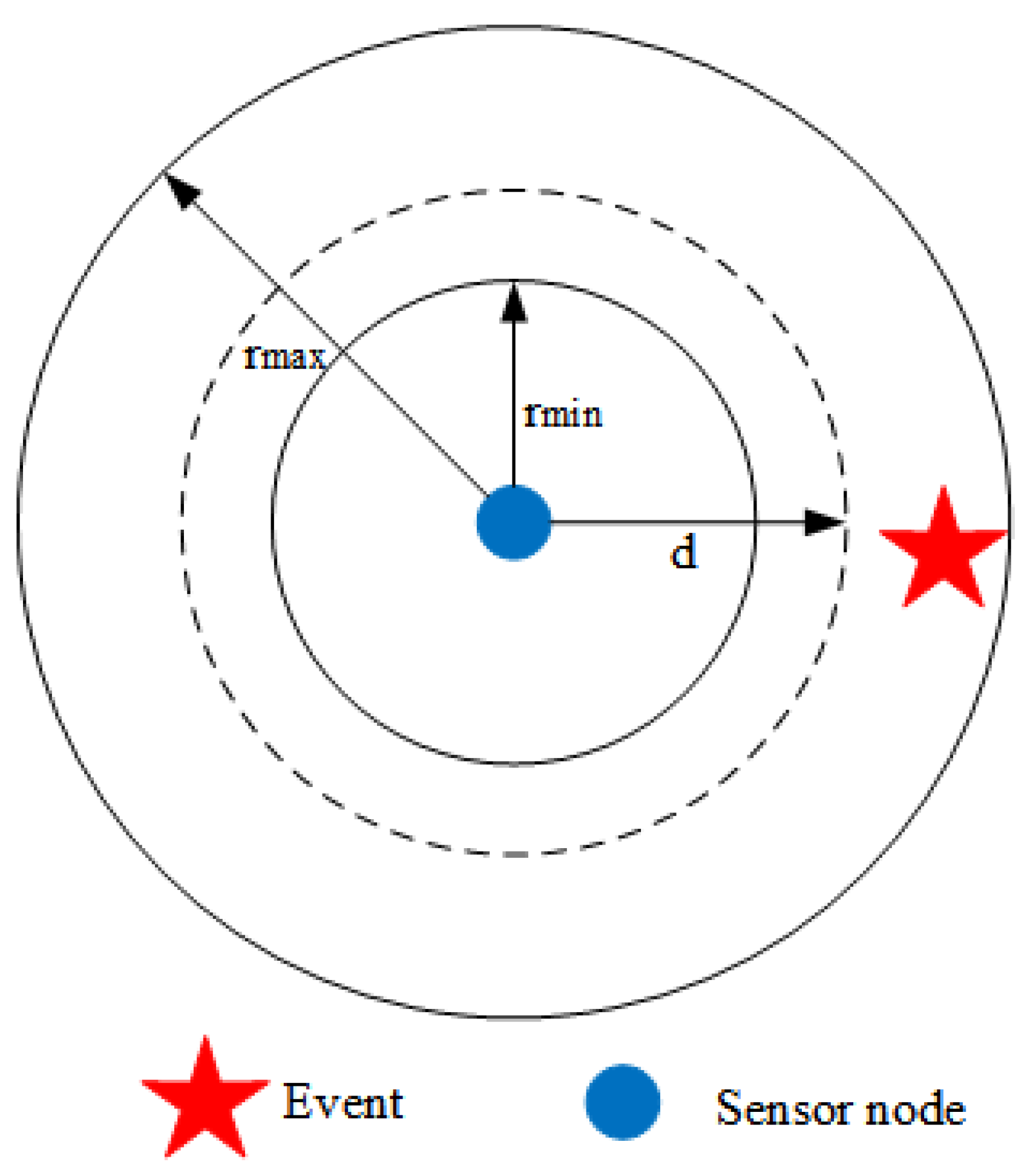
| d | Distance between sensor and event |
| r | Sensing radius |
| Minimum sensing radius | |
| Maximum sensing radius | |
| Detection accuracy | |
| Metrics of detection ability | |
| e | Energy depletion for sensing |
| Energy depletion of sensing in sleep duration | |
| Energy depletion of sensing in working duration | |
| Static power loss in sleep mode | |
| Static power loss in working mode | |
| Coefficient of energy depletion growing with distance | |
| Changeable power scaling parameter for the sensing circuit | |
| Step-size increasing factor | |
| Step-size diminishing factor | |
| N | Number of sensors |
| The sign function | |
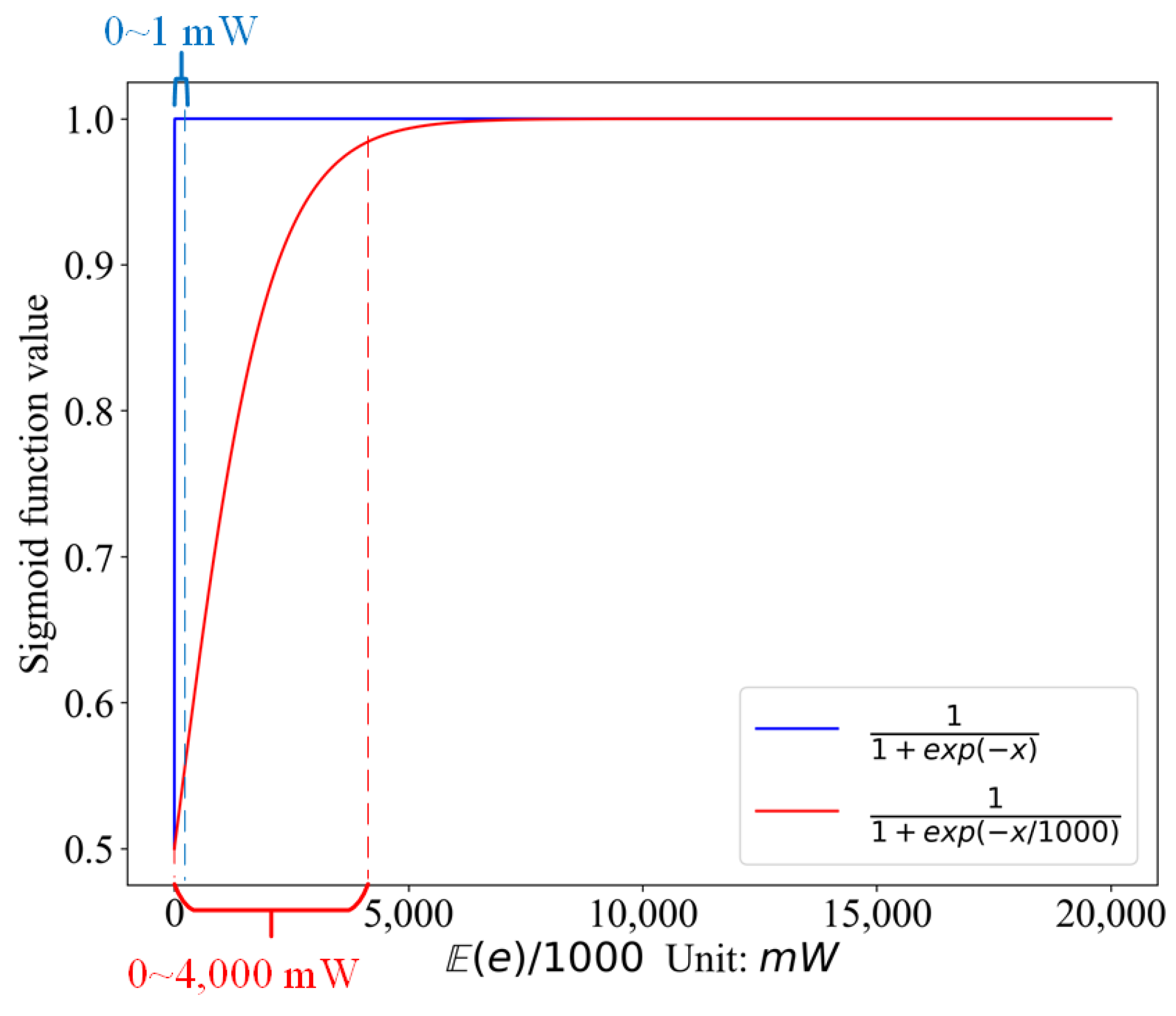
| The logistic Sigmoid function |
| FTO | Heuristic Algorithms | |
|---|---|---|
| Parameters | simple | many, hard to determine |
| Imitation of nature | phototropism | swarm intelligence |
| Characteristic | competitive elimination alternate search golden ratio search | random search based on probability |
| Global search capability | strong | prone to be trapped in local optimum |
| Convergence speed | fast | slow |
| Resources footprint | low | high |
| FTOS | Other Scheduling Strategies | ||
|---|---|---|---|
| Assumptions | Time synchronization | no | yes |
| Node density | no requirement | high | |
| Transmission radii | tunable | untunable | |
| Node location | movable | immovable | |
| Adaptability | strong | weak | |
| Deployment | easy | difficult | |
| Parameter | Value |
|---|---|
| Product model | E3F-DS100P1 |
| Operating voltage | DC 6~36 V |
| Operating current | 200 mA |
| Response frequency | 50 Hz |
| Sensing object | Any opaque object |
| Sensing radius | 10~100 cm, adjustable |
| Function | Form |
|---|---|
| Polynomial function | |
| Double-exponential function | |
| Checkmark function |
| Cases | Polynomial Function | Double-Exponential Function | Checkmark Function |
|---|---|---|---|
| and | 0.87 | 0.93 | 0.35 |
| and | 0.83 | 0.80 | 0.56 |
| and | 0.73 | 0.32 | 0.46 |
| and | 0.54 | 0.76 | 0.93 |
| Algorithm | Parameter | Value |
|---|---|---|
| Particle Swarm Optimization (PSO) | Population | 20 |
| Cognitive ratio | 2 | |
| Social coefficient | 2 | |
| Inertia weight | 0.4~0.9 | |
| Genetic Algorithm (GA) | Population | 100 |
| Point mutation | 0.01 | |
| Hoist mutation | 0.4 | |
| Parsimony coefficient | 0.01 | |
| Learning rate | 0.05~0.5 | |
| Comprehensive Learning Particle Swarm Optimization (CLPSO) | Population | 20 |
| Cognitive ratio | 2 | |
| Social coefficient | 2 | |
| Inertia weight | 0.4~0.9 | |
| Differential Evolution (DE) | Population | 20 |
| Scaling factor | 0.6 | |
| Crossover rate | 0.8 | |
| Artificial Bee Colony (ABC) | Followers | 50 |
| Scouters | 20 | |
| Employed foragers | 1 | |
| Fibonacci Tree Optimization (FTO) | Nested branch depth | 2 |
| Total branch depth | 6 | |
| Search space | [0,1] | |
| Max iterations | 1000 | |
| Precision | 0.001 |
| Algorithm | Iter = 10 | Iter = 50 | Iter = 200 | Iter = 500 | ||||||||
|---|---|---|---|---|---|---|---|---|---|---|---|---|
| PSO | 0.65 | 0.57 | 0.165 | 0.67 | 0.71 | 0.11 | 0.55 | 0.75 | 0.34 | 0.56 | 0.59 | 0.65 |
| GA | 0.87 | 0.57 | 0.2 | 0.76 | 0.38 | 0.6 | 0.57 | 0.56 | 0.13 | 0.55 | 0.55 | 0.65 |
| CLPSO | 0.52 | 0.72 | 0.4 | 0.49 | 0.18 | 0.74 | 0.56 | 0.75 | 0.9 | 0.54 | 0.15 | 0.15 |
| DE | 0.67 | 0.57 | 0.37 | 0.67 | 0.78 | 0.56 | 0.5 | 0.44 | 0.15 | 055 | 0.65 | 0.65 |
| ABC | 0.63 | 0.57 | 0.38 | 0.58 | 0.51 | 0.17 | 0.49 | 0.45 | 0.65 | 0.49 | 0.65 | 0.5 |
| FTO | 0.52 | 0.74 | 0.56 | 0.45 | 0.18 | 0.86 | 0.45 | 0.8 | 0.13 | 0.45 | 0.175 | 0.175 |
Publisher’s Note: MDPI stays neutral with regard to jurisdictional claims in published maps and institutional affiliations. |
© 2021 by the authors. Licensee MDPI, Basel, Switzerland. This article is an open access article distributed under the terms and conditions of the Creative Commons Attribution (CC BY) license (https://creativecommons.org/licenses/by/4.0/).
Share and Cite
Wu, L.; Cai, H. Energy-Efficient Adaptive Sensing Scheduling in Wireless Sensor Networks Using Fibonacci Tree Optimization Algorithm. Sensors 2021, 21, 5002. https://doi.org/10.3390/s21155002
Wu L, Cai H. Energy-Efficient Adaptive Sensing Scheduling in Wireless Sensor Networks Using Fibonacci Tree Optimization Algorithm. Sensors. 2021; 21(15):5002. https://doi.org/10.3390/s21155002
Chicago/Turabian StyleWu, Liangshun, and Hengjin Cai. 2021. "Energy-Efficient Adaptive Sensing Scheduling in Wireless Sensor Networks Using Fibonacci Tree Optimization Algorithm" Sensors 21, no. 15: 5002. https://doi.org/10.3390/s21155002
APA StyleWu, L., & Cai, H. (2021). Energy-Efficient Adaptive Sensing Scheduling in Wireless Sensor Networks Using Fibonacci Tree Optimization Algorithm. Sensors, 21(15), 5002. https://doi.org/10.3390/s21155002