
Measurement and Estimation of Spectral Sensitivity Functions for Mobile Phone Cameras


Abstract
:1. Introduction
2. Measurement of Spectral Sensitivity Functions
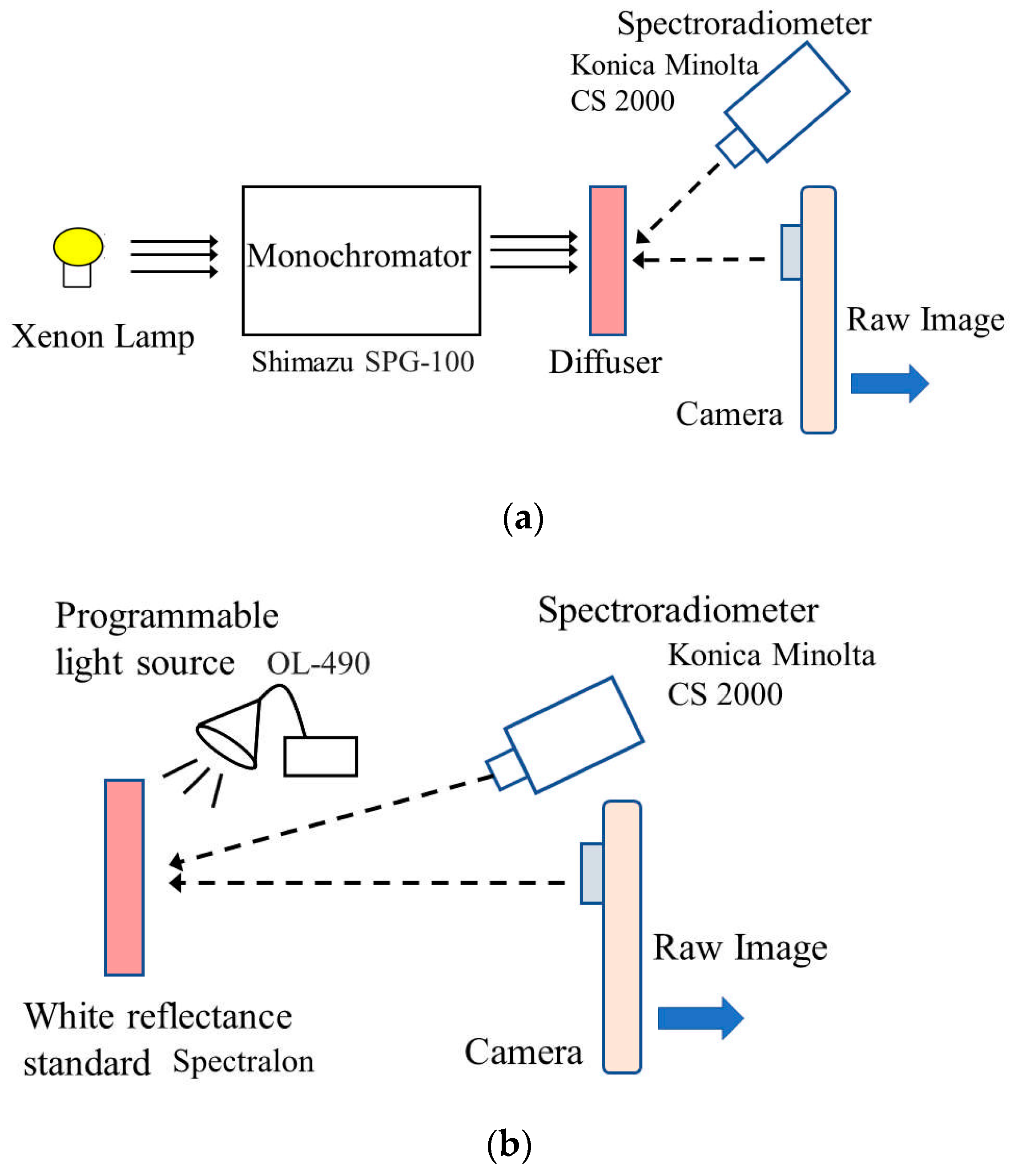
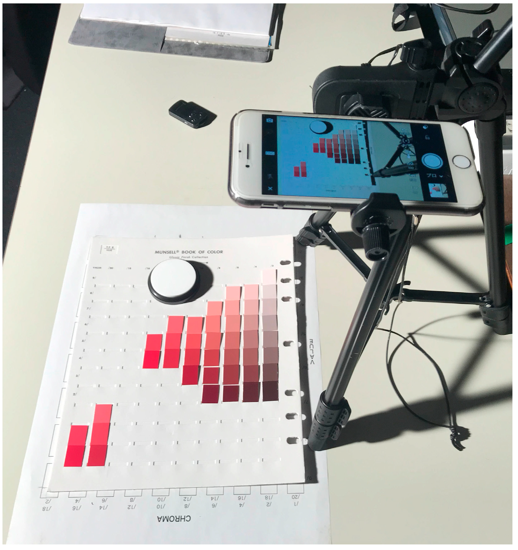
2.1. Measurement Setup
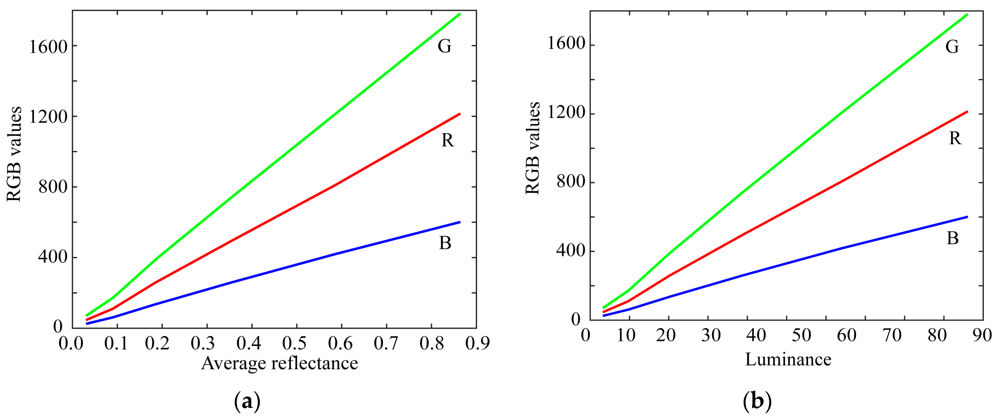
- (a)
- Linearity
- (b)
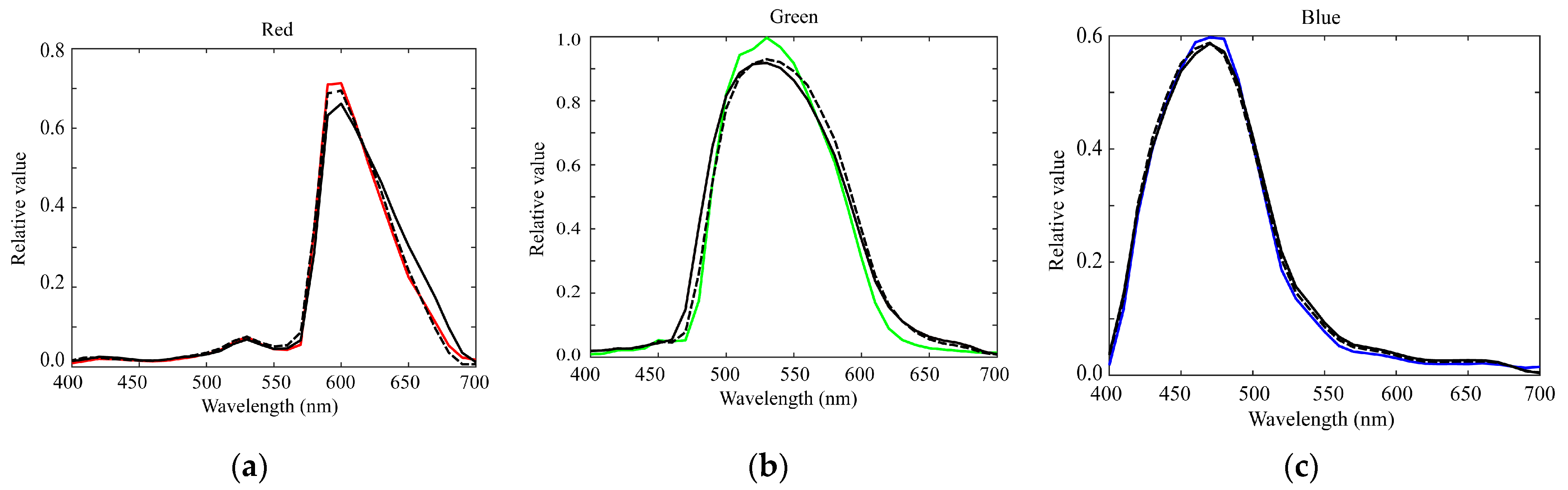
- Spectral response
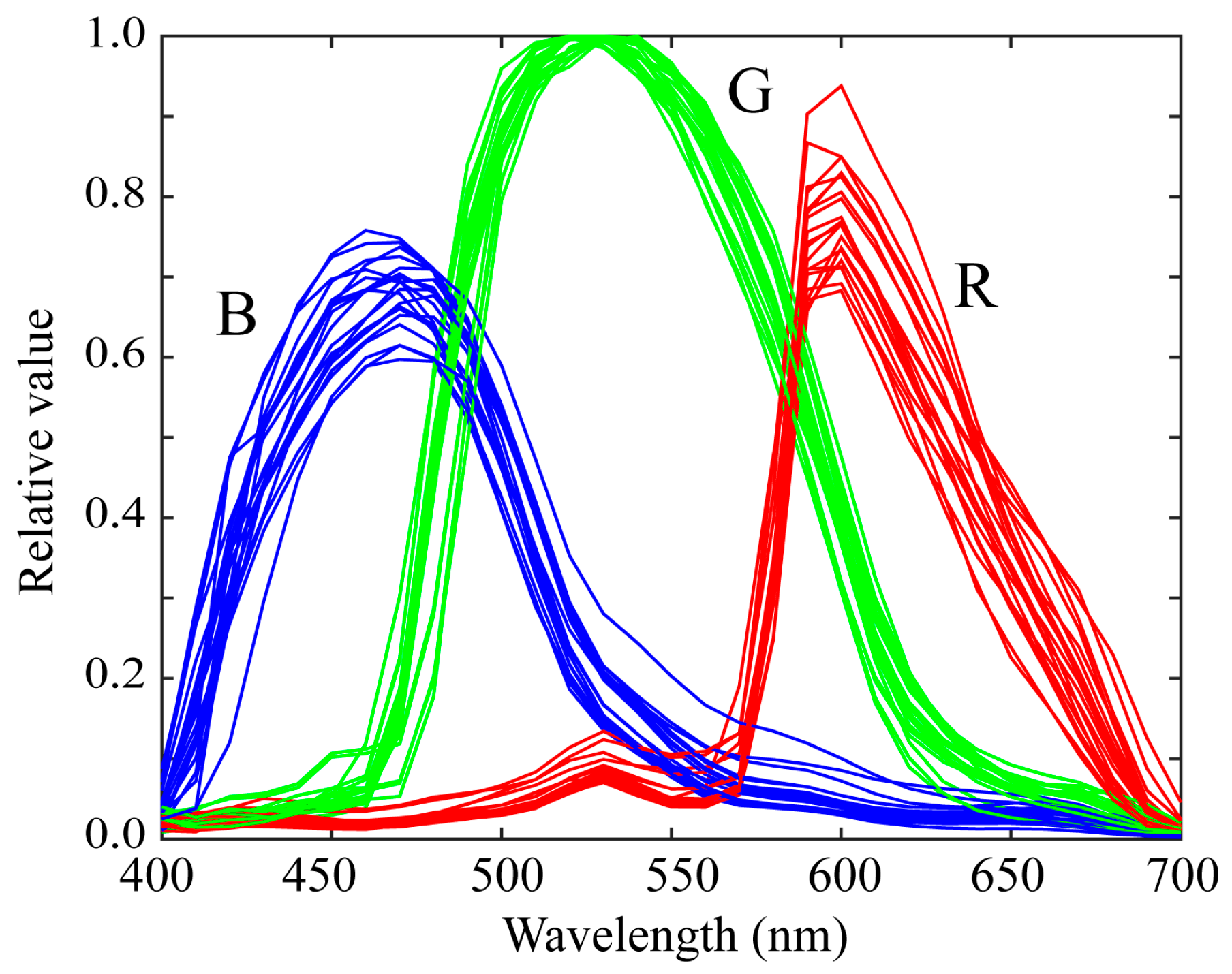
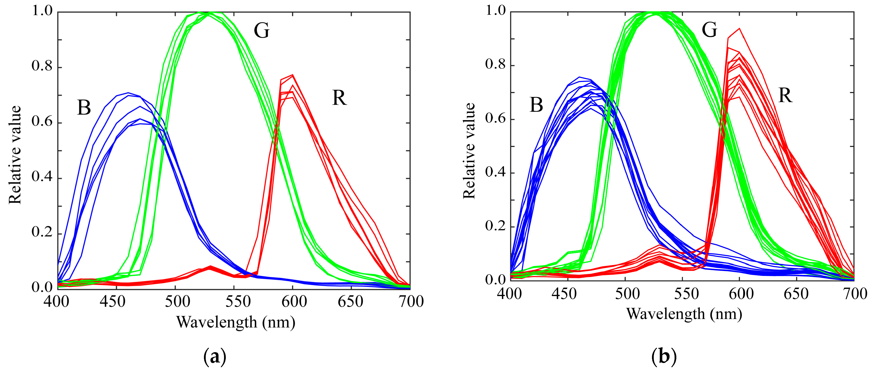
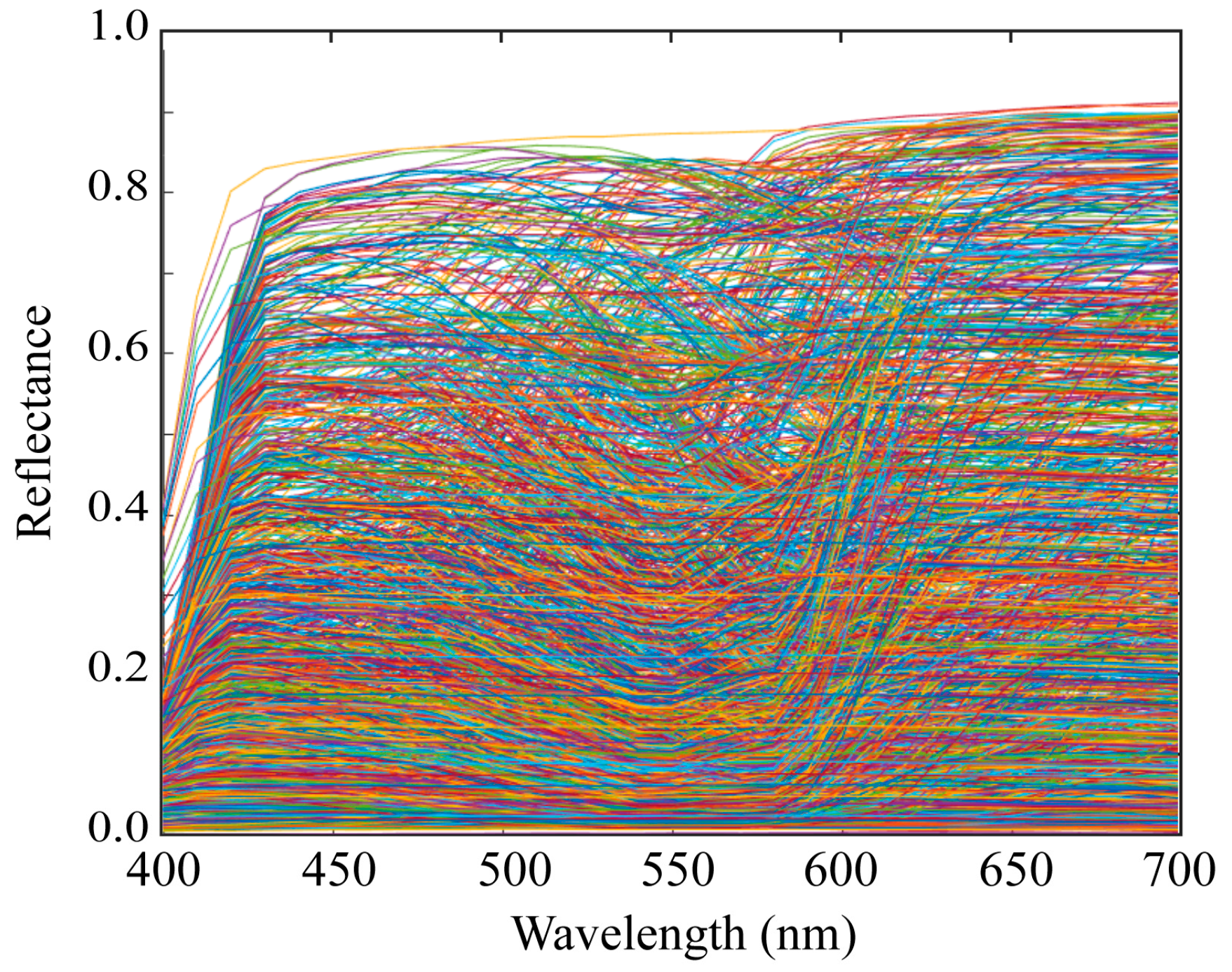
2.2. Spectral Sensitivity Database
3. Feature Analysis of Spectral Sensitivity Functions
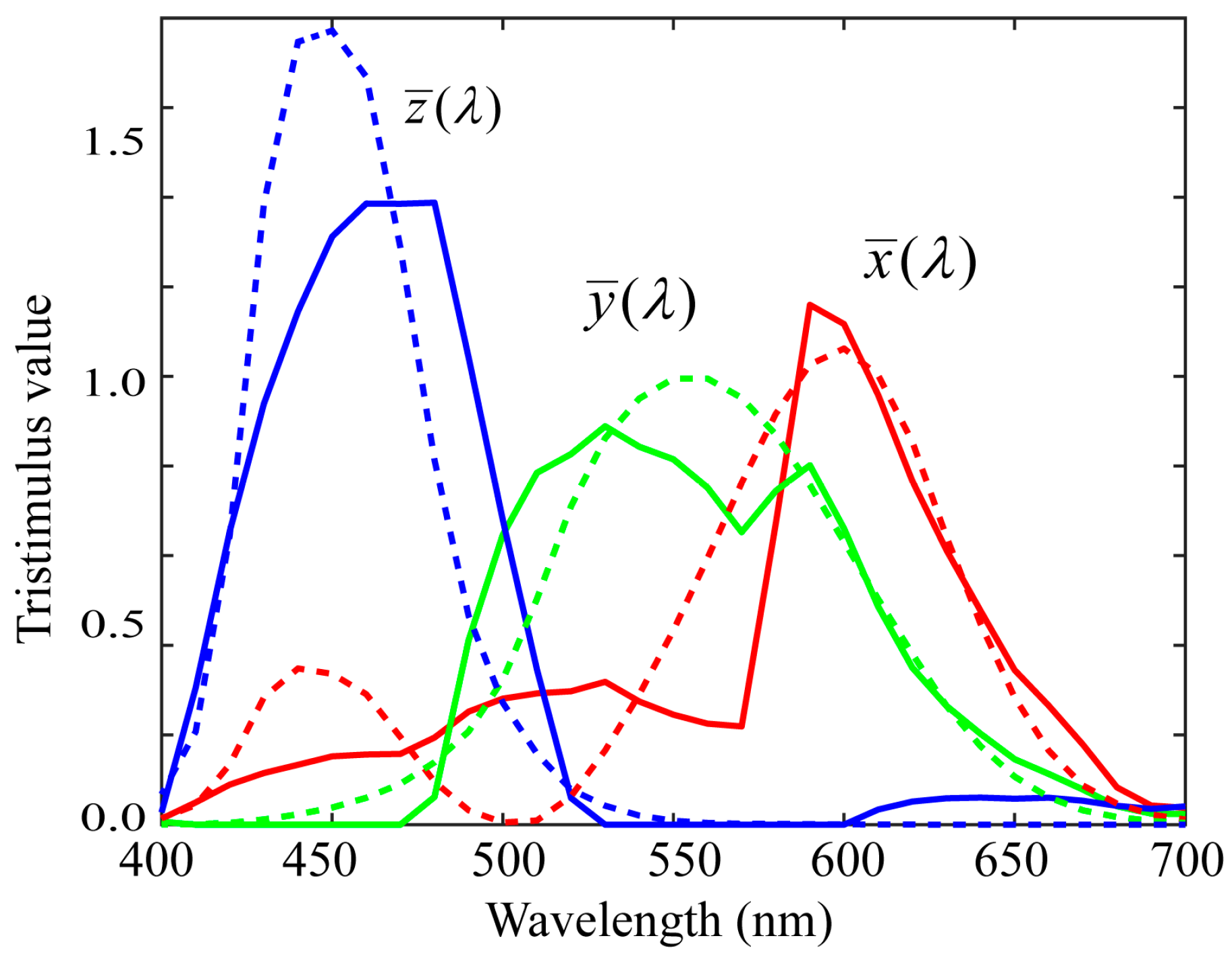
3.1. Fitting to Color-Matching Functions
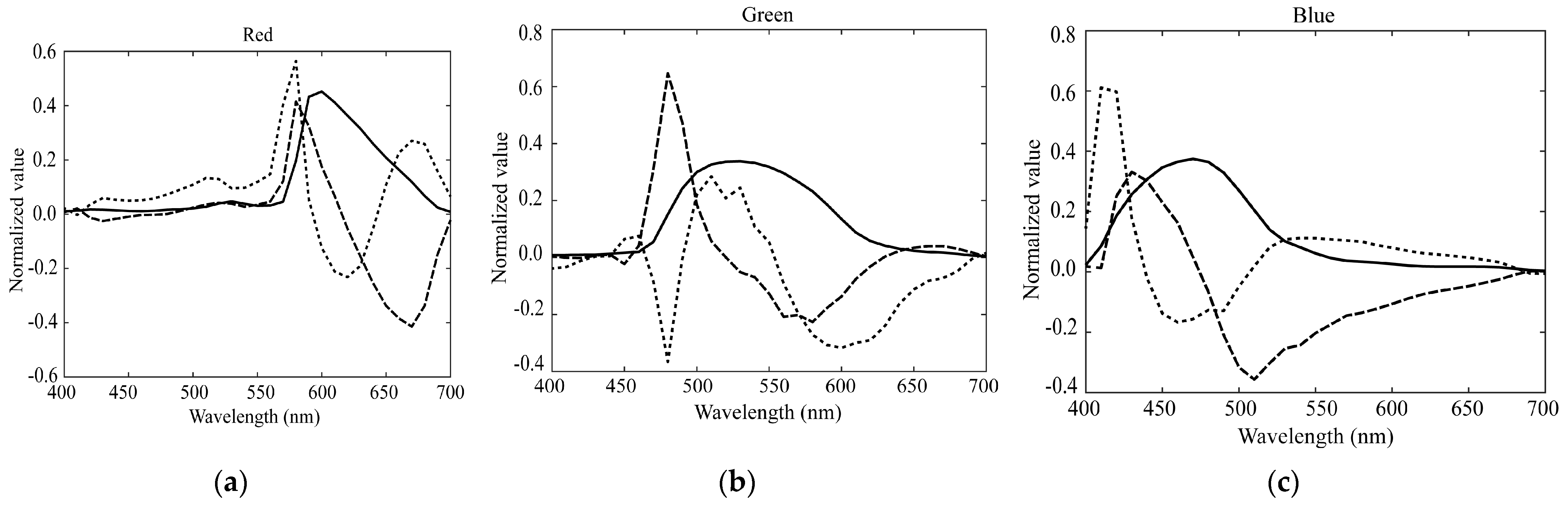
3.2. PCA Analysis
4. Estimation of Spectral Sensitivity Functions
4.1. Normal Method Using Color Samples
4.2. Proposed Method Based on Color Samples and Spectral Features
5. Experimental Results
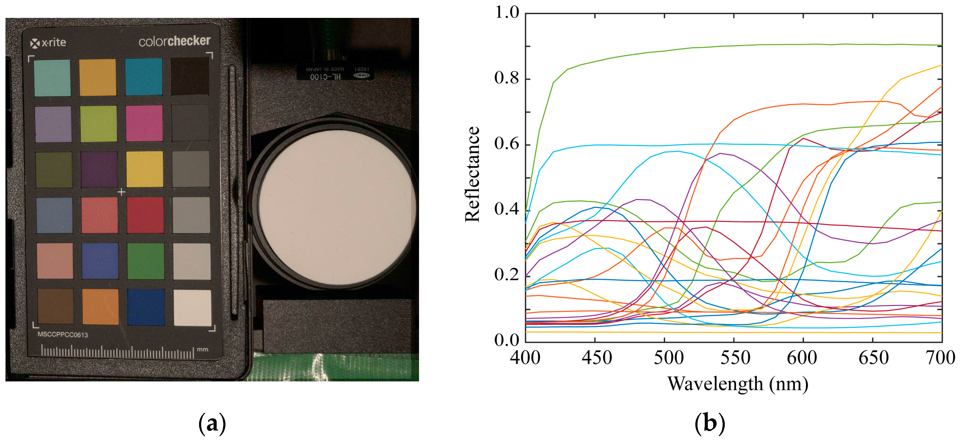
5.1. Experimental Setup
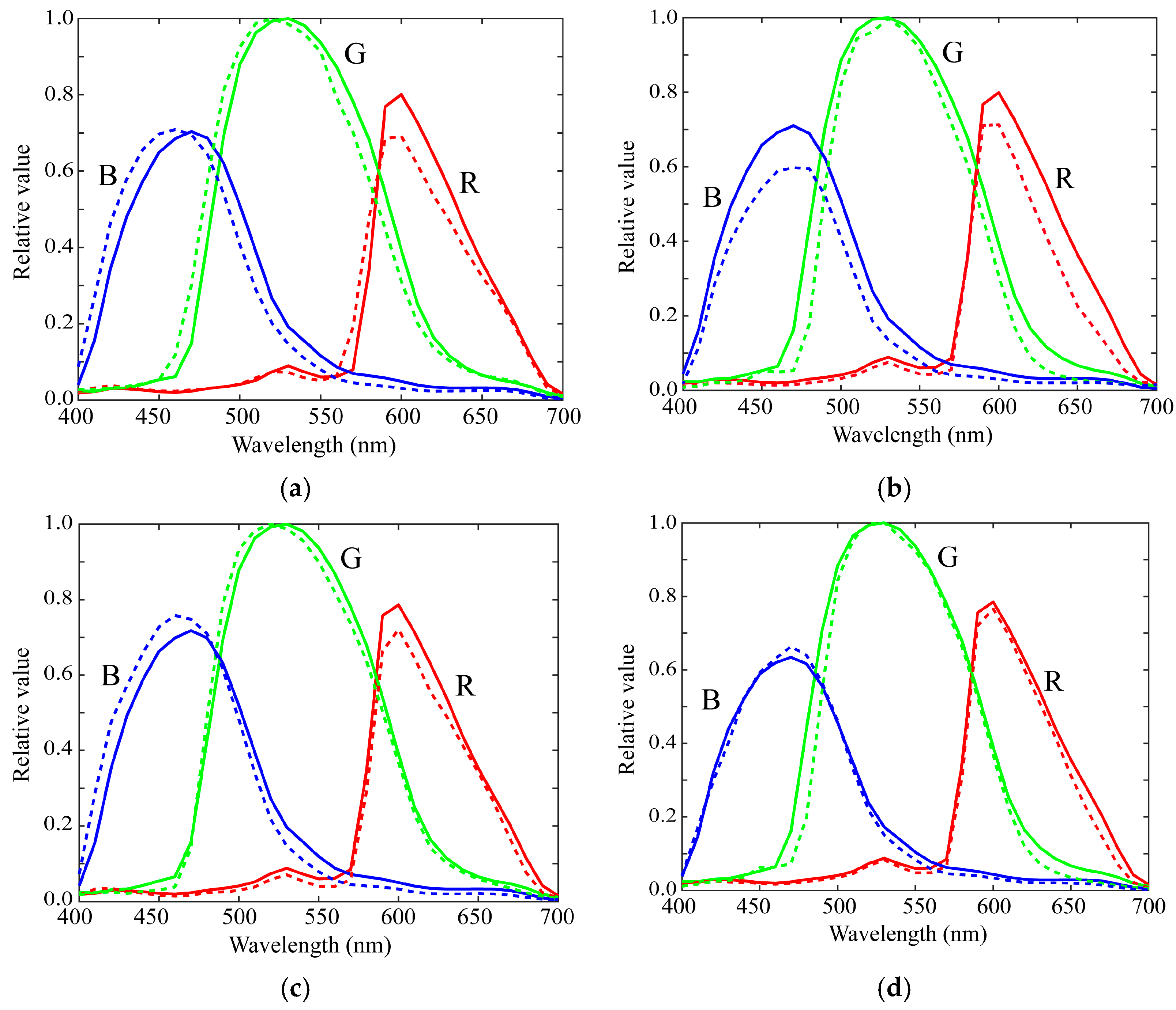
5.2. Validation of the Measured Spectral Sensitivities
5.3. Estimation Results by the Normal Method
5.4. Estimation Results by the Proposed Method
5.5. Reflectance Estimation Validation
6. Discussion
7. Conclusions
Author Contributions
Funding
Acknowledgments
Conflicts of Interest
References
- Statista. Number of Smartphone Subscriptions Worldwide from 2016 to 2026. Available online: https://www.statista.com/statistics/330695/number-of-smartphone-users-worldwide (accessed on 22 July 2021).
- Rateni, G.; Dario, P.; Cavallo, F. Smartphone-based food diagnostic technologies: A review. Sensors 2017, 17, 1453. [Google Scholar] [CrossRef]
- McGonigle, A.J.S.; Wilkes, T.C.; Pering, T.D.; Willmott, J.R.; Cook, J.M.; Mims, F.M.; Parisi, A.V. Smartphone spectrometers. Sensors 2018, 18, 223. [Google Scholar] [CrossRef] [PubMed] [Green Version]
- Burggraa, O.; Perduijn, A.B.; van Hek, R.F.; Schmidt, N.; Keller, C.U.; Snik, F. A universal smartphone add-on for portable spectroscopy and polarimetry: iSPEX 2. In Micro- and Nanotechnology Sensors, Systems, and Applications XII; International Society for Optics and Photonics: Bellingham, WA, USA, 2020; Volume 11389, p. 113892K. [Google Scholar] [CrossRef]
- Vora, P.L.; Farrell, J.E.; Tietz, J.D.; Brainard, D.H. Image capture: Simulation of sensor responses from hyperspectral images. IEEE Trans. Image Process. 2001, 10, 307–316. [Google Scholar] [CrossRef] [PubMed]
- Farrell, J.E.; Catrysse, P.B.; Wandell, B.A. Digital camera simulation. Applied Opt. 2012, 51, A80–A90. [Google Scholar] [CrossRef] [PubMed]
- Berra, E.; Gibson-Poole, S.; MacArthur, A.; Gaulton, R.; Hamilton, A. Estimation of the spectral sensitivity functions of un-modified and modified commercial off-shelf digital cameras to enable their use as a multispectral imaging system for UAVS. In Proceedings of the International Conference Unmanned Aer. Veh. Geomat, Toronto, ON, Canada, 30 August–2 September 2015; pp. 207–214. [Google Scholar] [CrossRef] [Green Version]
- Darrodi, M.M.; Finlayson, G.D.; Good-man, T.; Mackiewicz, M. A reference data set for camera spectral sensitivity estimation. J. Opt. Soc. Am. A 2014, 32, 381–391. [Google Scholar] [CrossRef] [PubMed] [Green Version]
- Camera Spectral Sensitivity Database. Available online: http://www.gujinwei.org/research/camspec/camspec_database.txt (accessed on 21 July 2021).
- Nakamura, J. Image Sensors and Signal Processing for Digital Still Cameras; CRC Press: Boca Raton, FL, USA, 2006. [Google Scholar]
- Hubel, P.M.; Sherman, D.; Farrell, J.E. A comparison of methods of sensor spectral sensitivity estimation. In Color and Imaging Conference; Society for Imaging Science and Technology: Scottsdale, AZ, USA, 15–18 November 1994; Volume 1994, pp. 45–48. [Google Scholar]
- Hardeberg, J.Y.; Bretel, H.; Schmitt, F.J.M. Spectral characterization of electronic cameras. In Proceedings of the Electronic Imaging: Processing, Printing, and Publishing in Color, Zurich, Switzerland, 18–20 May 1998; Volume 3499, pp. 100–109. [Google Scholar] [CrossRef]
- DiCarlo, J.M.; Montgomery, G.E.; Trovinger, S.W. Emissive chart for imager calibration. In Color and Imaging Conference; Society for Imaging Science and Technology: Scottsdale, AZ, USA, 9–12 November 2004; pp. 295–301. [Google Scholar]
- Han, S.; Matsushita, Y.; Sato, I.; Okabe, T.; Sato, Y. Camera spectral sensitivity estimation from a single image under unknown illumination by using fluorescence. In Proceedings of the IEEE Conference on Computer Vision and Pattern Recognition (CVPR), Providence, RI, USA, 18–20 June 2012; pp. 805–812. [Google Scholar] [CrossRef] [Green Version]
- Zhu, J.; Xie, X.; Liao, N.; Zhang, Z.; Wu, W.; Lv, L. Spectral sensitivity estimation of trichromatic camera based on orthogonal test and window filtering. Opt. Express 2020, 28, 28085–28100. [Google Scholar] [CrossRef] [PubMed]
- Jiang, J.; Liu, D.; Gu, J.; Susstrunk, S. What is the space of spectral sensitivity functions for digital color cameras. In Proceedings of the IEEE Workshop on the Applications of Computer Vision, Tampa, FL, USA, 15–17 January 2013; pp. 168–179. [Google Scholar] [CrossRef] [Green Version]
- Finlayson, G.; Darrodi, M.M.; Mackiewicz, M. Rank-based camera spectral sensitivity estimation. J. Opt. Soc. Am. A 2016, 33, 589–599. [Google Scholar] [CrossRef] [PubMed] [Green Version]
- Ji, Y.; Kwak, Y.; Park, S.M.; Kim, Y.L. Compressive recovery of smartphone RGB spectral sensitivity functions. Opt. Express 2021, 29, 11947–11961. [Google Scholar] [CrossRef] [PubMed]
- Bongiorno, D.L.; Bryson, M.; Dansereau, D.G.; Williams, S.B. Spectral characterization of COTS RGB cameras using a linear variable edge filter. In Proceedings of the SPIE 8660 Digital Photography IX; Sampat, N., Battiato, S., Eds.; International Society for Optics and Photonics: Burlingame, CA, USA, 3–7 February 2013; p. 86600N. [Google Scholar] [CrossRef]
- Burggraaff, O.; Schmidt, N.; Zamorano, J.; Pauly, K.; Pascual, S.; Tapia, C.; Spyrakos, E.; Snik, F. Standardized spectral and radiometric calibration of consumer cameras. Opt. Express 2019, 27, 19075–19101. [Google Scholar] [CrossRef] [PubMed] [Green Version]
- Adobe Systems Incorporated. Digital Negative (DNG) Specification, Version 1.4.0.0.; Adobe Systems Incorporated: San Jose, CA, USA, 2012. [Google Scholar]
- Bazhyna, A.; Gotchev, A.; Egiazarian, K. Near-lossless compression algorithm for Bayer pattern color filter arrays. In Digital Photography; International Society for Optics and Photonics: Burlingame, CA, USA, 2005; Volume 5678, pp. 198–209. [Google Scholar] [CrossRef]
- Tominaga, S.; Nishi, S.; Ohtera, R. Estimating spectral sensitivities of a smartphone camera. In Proceedings of the IS&T International Symposium Electronic Imaging, Online, 11–21 January 2021; Volume XXVI, p. COLOR-223. [Google Scholar]
- Tominaga, S.; Horiuchi, T. Spectral imaging by synchronizing capture and illumination. J. Opt. Soc. Am. A 2012, 29, 1764–1775. [Google Scholar] [CrossRef] [PubMed]
- Ohta, N.; Robertson, A.R. Measurement and Calculation of Colorimetric Values. In Colorimetry: Fundamentals and Applications; John Wiley & Sons, Ltd.: Hoboken, NJ, USA, 2005; Chapter 5. [Google Scholar]
- Golub, G.H.; van Loan, C.F. Matrix Computations, 4th ed.; Johns Hopkins University: Baltimore, MD, USA, 2013. [Google Scholar]
- Parkkinen, J.; Hallikainen, J.; Jaaskelainen, T. Characteristic spectra of Munsell colors. J. Opt. Soc. Am. A 1989, 6, 318–322. [Google Scholar] [CrossRef]
- Tominaga, S. Multichannel vision system for estimating surface and illuminant functions. J. Opt. Soc. Am. A 1996, 13, 2163–2173. [Google Scholar] [CrossRef]
- Munsell Products. Available online: https://www.modeinfo.com/en/Munsell-Products/ (accessed on 21 July 2021).
- ColorChecker Passport Photo 2. Available online: https://xritephoto.com/ph_product_overview.aspx?id=2572&catid=158 (accessed on 21 July 2021).
- Haneishi, H.; Hasegawa, T.; Hosoi, A.; Yokoyama, Y.; Tsumura, N.; Miyake, Y. System design for accurately estimating the spectral reflectance of art paintings. Appl. Opt. 2000, 39, 6621–6632. [Google Scholar] [CrossRef] [PubMed] [Green Version]
- Shimano, N. Recovery of spectral reflectances of objects being imaged without prior knowledge. IEEE Trans. Image Process. 2006, 15, 1848–1856. [Google Scholar] [CrossRef] [PubMed]
- Shimano, N.; Terai, K.; Hironaga, M. Recovery of spectral reflectances of objects being imaged by multispectral cameras. J. Opt. Soc. Am. A 2007, 24, 3211–3219. [Google Scholar] [CrossRef] [PubMed]
- Stigell, P.; Miyata, K.; Hauta-Kasari, M. Wiener estimation method in estimating of spectral reflectance from RGB image. Pattern Recognit. Image Anal. 2007, 17, 233–242. [Google Scholar] [CrossRef]
- Murakami, Y.; Fukura, K.; Yamaguchi, M.; Ohyama, N. Color reproduction from low-SNR multispectral images using spatio-spectral Wiener estimation. Opt. Express 2008, 16, 4106–4120. [Google Scholar] [CrossRef] [PubMed]
- Urban, P.; Rosen, M.R.; Berns, R.S. A Spatially Adaptive Wiener Filter for Reflectance Estimation. In Proceedings of the 16th Color Imaging Conference, Portland, OR, USA, 10–14 November 2008; pp. 279–284. [Google Scholar]
- Nahavandi, A.M. Noise segmentation for improving performance of Wiener filter method in spectral reflectance estimation. Color Res. Appl. 2018, 43, 341–348. [Google Scholar] [CrossRef]
- Tominaga, S.; Matsuura, A.; Horiuchi, T. Spectral analysis of omnidirectional illumination in a natural scene. J. Imaging Sci. Technol. 2010, 54, 040502-1–040502-9. [Google Scholar] [CrossRef]


| Manufacturer | Model | Image Sensor |
|---|---|---|
| Apple | iPhone 6s | Sony IMX315 |
| Apple | iPhone SE | Sony IMX315 |
| Apple | iPhone 8 | Sony IMX315 |
| Apple | iPhone X | Sony IMX315 |
| Apple | iPhone 11 | Sony IMX503 |
| Apple | iPhone 12 Pro MAX | Sony IMX603 |
| HUAWEI | P10 lite | Sony IMX214 |
| HUAWEI | nova lite 2 | Unknown |
| Samsung | Galaxy S7 edge | Samsung ISOCELL S5K2L1 |
| Samsung | Galaxy S9 | Samsung ISOCELL S5K2L3 |
| Samsung | Galaxy Note10+ | Samsung ISOCELL S5K2L4 |
| Samsung | Galaxy S20 | Samsung ISOCELL S5KGW2 |
| SHARP | AQUOS sense3 lite | Unknown |
| SHARP | AQUOS R5G | Infineon Technologies IRS2381C |
| Xiaomi | Mi Mix 2s | Samsung ISOCELL S5K3M3 |
| Xiaomi | Redmi Note 9S | Samsung ISOCELL S5KGM2 |
| Sony | Xperia 1 II | Sony IMX557 |
| Sony | Xperia 5 II | Sony IMX557 |
| Fujitsu | arrows NX9 | Unknown |
| Pixel 4 | Sony IMX363 |
| Color Difference | Model | |||
|---|---|---|---|---|
| iPhone 6s | iPhone 8 | P10 Lite | Galaxy S7 Edge | |
| 0.01530 | 0.02046 | 0.01772 | 0.01689 | |
| RMSE | Model | |||
|---|---|---|---|---|
| iPhone 6s | iPhone 8 | P10 Lite | Galaxy S7 Edge | |
| L = 1 | 0.05577 | 0.06597 | 0.03841 | 0.03779 |
| L = 2 | 0.07167 | 0.10714 | 0.05741 | 0.03946 |
| L = 3 | 0.06378 | 0.07310 | 0.06816 | 0.04277 |
| Measurement 1 | Measurement 2 | Estimation 1 | Estimation 2 | |
|---|---|---|---|---|
| Average RMSE | 0.05241 | 0.05145 | 0.05201 | 0.05279 |
| Average LAB color difference | 7.055 | 6.082 | 6.973 | 6.749 |
Publisher’s Note: MDPI stays neutral with regard to jurisdictional claims in published maps and institutional affiliations. |
© 2021 by the authors. Licensee MDPI, Basel, Switzerland. This article is an open access article distributed under the terms and conditions of the Creative Commons Attribution (CC BY) license (https://creativecommons.org/licenses/by/4.0/).
Share and Cite
Tominaga, S.; Nishi, S.; Ohtera, R. Measurement and Estimation of Spectral Sensitivity Functions for Mobile Phone Cameras. Sensors 2021, 21, 4985. https://doi.org/10.3390/s21154985
Tominaga S, Nishi S, Ohtera R. Measurement and Estimation of Spectral Sensitivity Functions for Mobile Phone Cameras. Sensors. 2021; 21(15):4985. https://doi.org/10.3390/s21154985
Chicago/Turabian StyleTominaga, Shoji, Shogo Nishi, and Ryo Ohtera. 2021. "Measurement and Estimation of Spectral Sensitivity Functions for Mobile Phone Cameras" Sensors 21, no. 15: 4985. https://doi.org/10.3390/s21154985
APA StyleTominaga, S., Nishi, S., & Ohtera, R. (2021). Measurement and Estimation of Spectral Sensitivity Functions for Mobile Phone Cameras. Sensors, 21(15), 4985. https://doi.org/10.3390/s21154985