
Wheat Ear Recognition Based on RetinaNet and Transfer Learning

 ,
,
Abstract
:1. Introduction
2. Materials and Methods
2.1. Data Acquisition and Processing
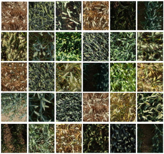
2.1.1. Global Wheat Data Acquisition
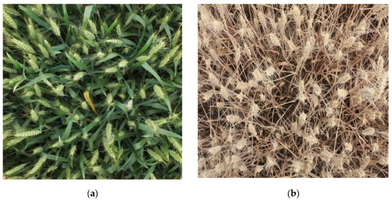
2.1.2. Digital Image Data Acquisition
2.1.3. Data Processing
- (1)
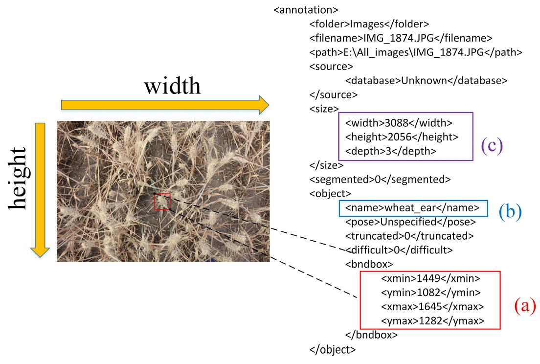
- Image marking
- (2)
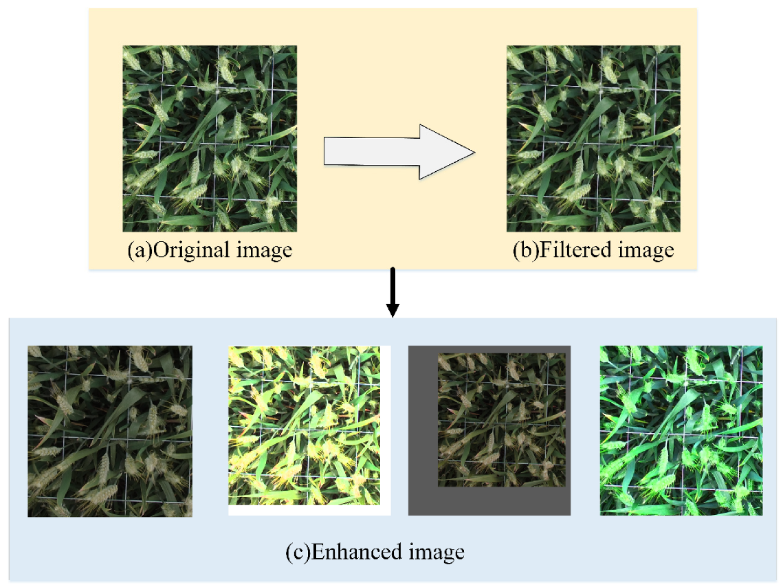
- Denoising and enhancement
2.2. Method
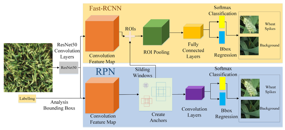
2.2.1. Faster R-CNN
- (1)
- Convolution layer.
- (2)
- RPN layer.
- (3)
- Region of Interest (ROI) pooling layer [14].
- (4)
- Recognition.
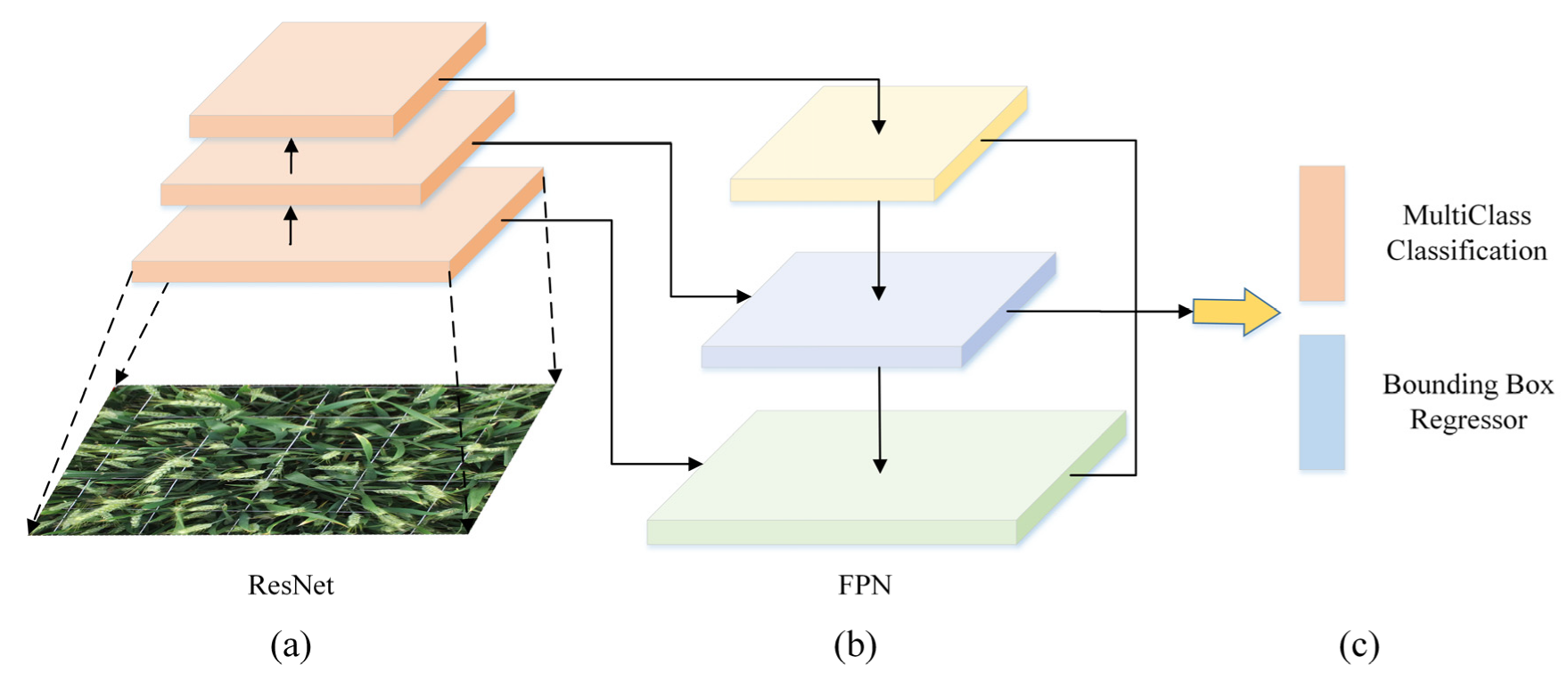
2.2.2. RetinaNet
2.2.3. Recognition Accuracy Evaluation Index
3. Results
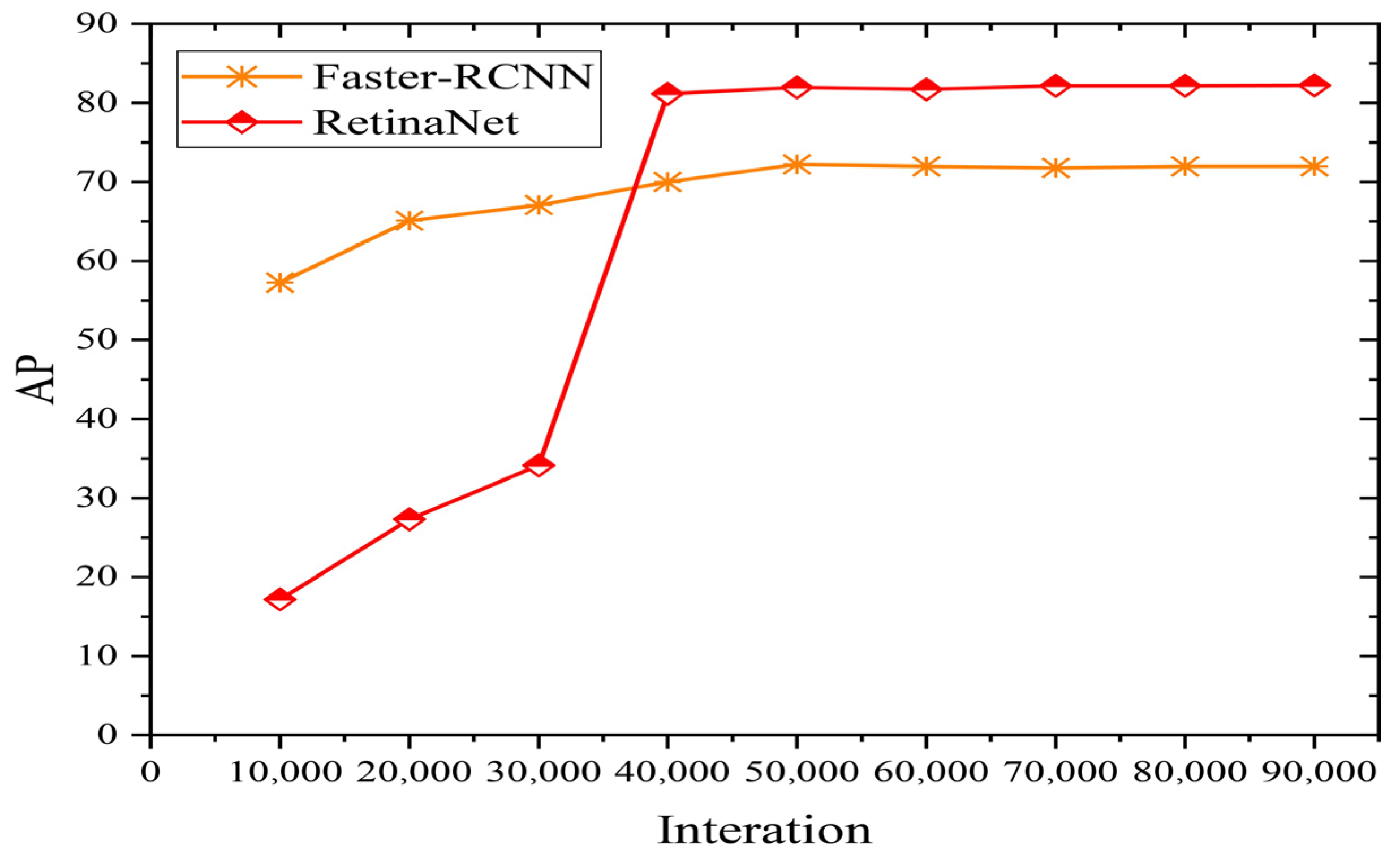
3.1. Analysis of the Recognition Results Obtained by Different Methods on the Global WHEAT Dataset
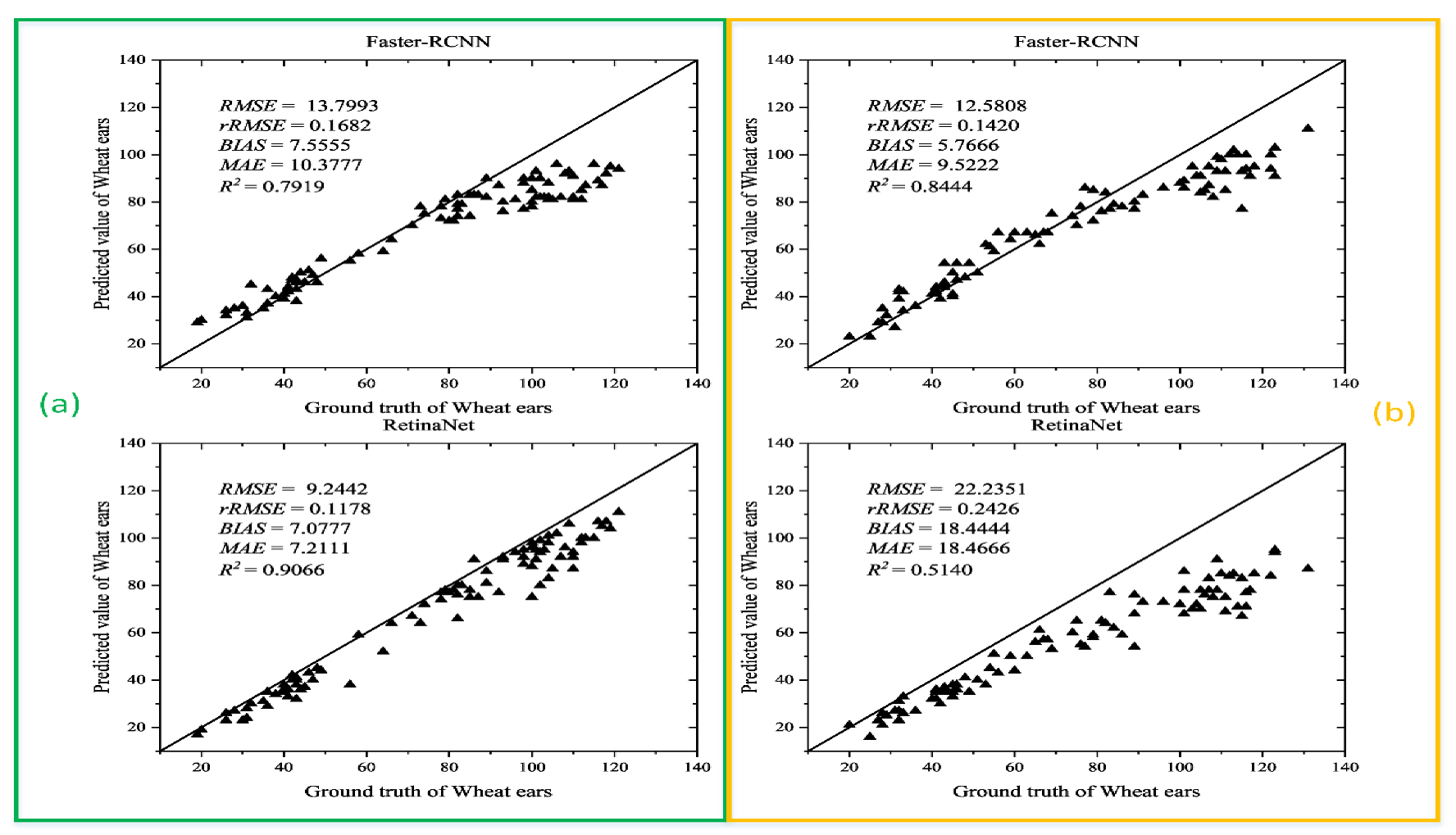
3.2. Results and Analysis of Wheat Ear Recognition Based on Transfer Learning
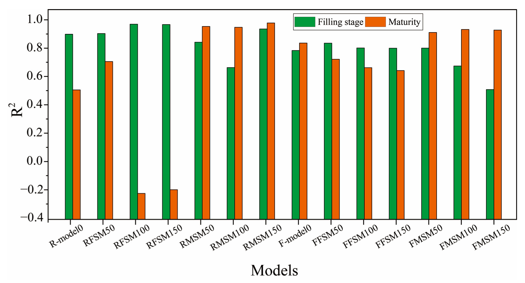
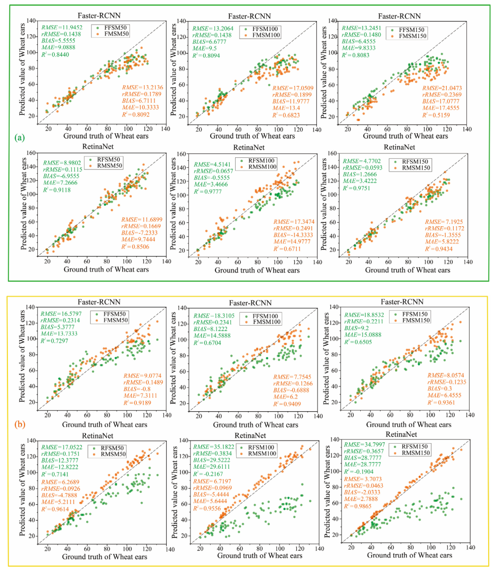
3.2.1. Recognition Results and Analysis of Different Numbers of Training Samples after Transfer Learning
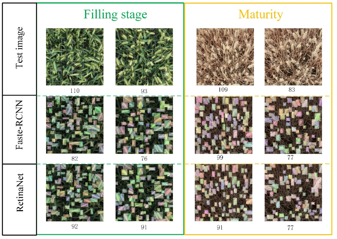
3.2.2. Recognition Results and Analysis of Transfer Learning in Different Growth Stages
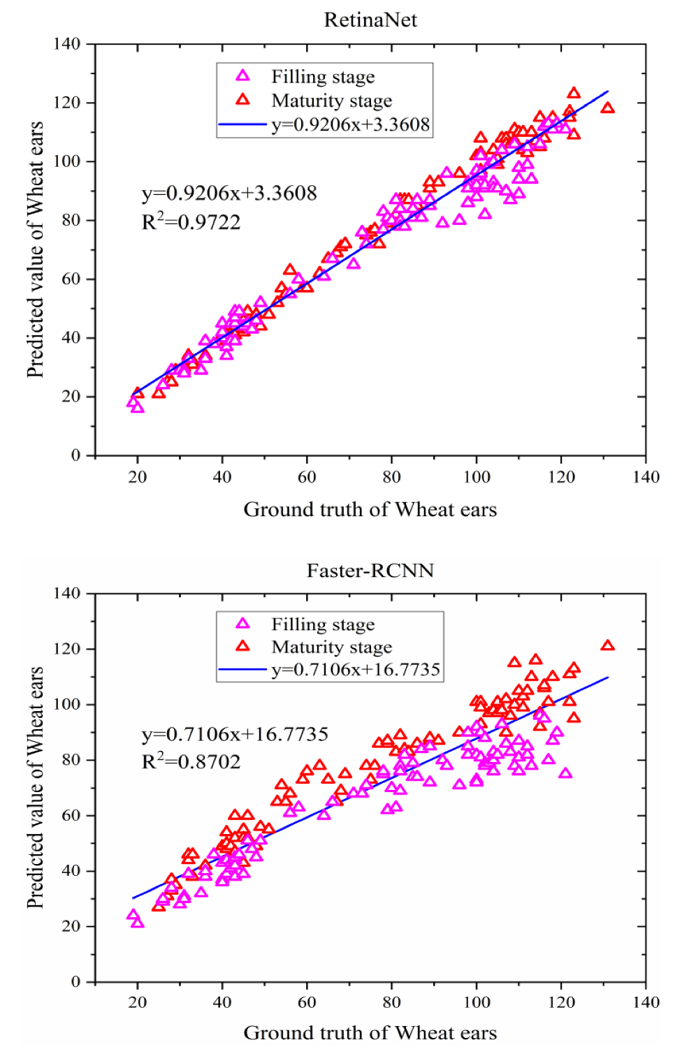
3.3. The Recognition Results and Analysis of RetinaNet
4. Discussion
5. Conclusions
Author Contributions
Funding
Institutional Review Board Statement
Informed Consent Statement
Data Availability Statement
Acknowledgments
Conflicts of Interest
References
- FAOSTAT. Available online: http://faostat3.fao.org/faostat-gateway/go/to/browse/Q/QC/E (accessed on 2 June 2021).
- Chen, C.; Frank, K.; Wang, T.; Wu, F. Global wheat trade and Codex Alimentarius guidelines for deoxynivalenol: A mycotoxin common in wheat. Glob. Food Secur. 2021, 29, 100538. [Google Scholar] [CrossRef]
- Powell, J.P.; Reinhard, S. Measuring the effects of extreme weather events on yields. Weather Clim. Extrem. 2016, 12, 69–79. [Google Scholar] [CrossRef] [Green Version]
- Gómez-Plana, A.G.; Devadoss, S. A spatial equilibrium analysis of trade policy reforms on the world wheat market. Appl. Econ. 2004, 36, 1643–1648. [Google Scholar] [CrossRef]
- Zhang, H.; Turner, N.C.; Poole, M.L.; Asseng, S. High ear number is key to achieving high wheat yields in the high-rainfall zone of south-western Australia. Aust. J. Agric. Res. 2007, 58, 21–27. [Google Scholar] [CrossRef]
- Gou, F.; van Ittersum, M.K.; Wang, G.; van der Putten, P.E.; van der Werf, W. Yield and yield components of wheat and maize in wheat–maize intercropping in the Netherlands. Eur. J. Agron. 2016, 76, 17–27. [Google Scholar] [CrossRef]
- Zhou, H.; Riche, A.B.; Hawkesford, M.J.; Whalley, W.R.; Atkinson, B.S.; Sturrock, C.J.; Mooney, S.J. Determination of wheat spike and spikelet architecture and grain traits using X-ray Computed Tomography imaging. Plant Methods 2021, 17, 26. [Google Scholar] [CrossRef] [PubMed]
- Hasan, M.M.; Chopin, J.P.; Laga, H.; Miklavcic, S.J. Detection and analysis of wheat spikes using Convolutional Neural Networks. Plant Methods 2018, 14, 100. [Google Scholar] [CrossRef] [PubMed] [Green Version]
- Fernandez-Gallego, J.A.; Kefauver, S.C.; Gutiérrez, N.A.; Nieto-Taladriz, M.T.; Araus, J.L. Wheat ear counting in-field conditions: High throughput and low-cost approach using RGB images. Plant Methods 2018, 14, 22. [Google Scholar] [CrossRef] [Green Version]
- Dong, S.; Wang, P.; Abbas, K. A survey on deep learning and its applications. Comput. Sci. Rev. 2021, 40, 100379. [Google Scholar] [CrossRef]
- Jin, X.; Zarco-Tejada, P.; Schmidhalter, U.; Reynolds, M.P.; Hawkesford, M.J.; Varshney, R.K.; Yang, T.; Nie, C.H.; Li, Z.; Ming, B.; et al. High-throughput estimation of crop traits: A review of ground and aerial phenotyping platforms. IEEE Geosci. Remote Sens. Mag. 2021, 9, 200–231. [Google Scholar] [CrossRef]
- Lippitt, C.D.; Zhang, S. The impact of small unmanned airborne platforms on passive optical remote sensing: A conceptual perspective. Int. J. Remote Sens. 2018, 39, 4852–4868. [Google Scholar] [CrossRef]
- Mickinney, S.M.; Karthikesalingam, A.; Tse, D.; Kelly, C.J.; Shetty, S. Reply to: Transparency and reproducibility in artificial intelligence. Nature 2020, 586, E17–E18. [Google Scholar] [CrossRef]
- Ren, S.; He, K.; Girshick, R.; Sun, J. Faster R-CNN: Towards real-time object detection with region proposal networks. IEEE Trans. Pattern Anal. Mach. Intell. 2017, 39, 1137–1149. [Google Scholar] [CrossRef] [Green Version]
- Madec, S.; Jin, X.; Lu, H.; De Solan, B.; Liu, S.; Duyme, F.; Heritier, E.; Baret, F. Ear density estimation from high resolution RGB imagery using deep learning technique. Agric. For. Meteorol. 2019, 264, 225–234. [Google Scholar] [CrossRef]
- Girshick, R. Fast R-CNN. In Proceedings of the 2015 IEEE International Conference on Computer Vision (ICCV), Santiago, Chile, 7–13 December 2015; pp. 1440–1448. [Google Scholar]
- Redmon, J.; Divvala, S.; Girshick, R.; Farhadi, A. You Only Look Once: Unified, Real-Time Object Detection. In Proceedings of the IEEE Conference on Computer Vision and Pattern Recognition (CVPR), Las Vegas, NV, USA, 27–30 June 2016. [Google Scholar]
- Redmon, J.; Farhadi, A. Yolov3: An incremental improvement. arXiv 2018, arXiv:1804.02767. [Google Scholar]
- Lin, T.Y.; Goyal, P.; Girshick, R.; He, K.; Dollár, P. Focal Loss for Dense Object Detection. IEEE Trans. Pattern Anal. Mach. Intell. 2017, 99, 2999–3007. [Google Scholar]
- Liu, W.; Anguelov, D.; Erhan, D.; Szegedy, C.; Reed, S.; Fu, C.Y.; Berg, A.C. SSD: Single shot multibox detector. In Proceedings of the European Conference on Computer Vision, Amsterdam, The Netherlands, 8–16 October 2016; pp. 21–37. [Google Scholar]
- Lin, T.Y.; Dollár, P.; Girshick, R.; He, K.; Hariharan, B.; Belongie, S. Feature pyramid networks for object detection. In Proceedings of the IEEE Conference on Computer Vision and Pattern Recognition (CVPR), Honolulu, HI, USA, 21–26 July 2017; pp. 2117–2125. [Google Scholar]
- Wang, Y.; Wang, C.; Zhang, H.; Dong, Y.; Wei, S. Automatic Ship Detection Based on RetinaNet Using Multi-Resolution Gaofen-3 Imagery. Remote Sens. 2019, 11, 531. [Google Scholar] [CrossRef] [Green Version]
- Santos, A.; Marcato Junior, J.; de Andrade Silva, J.; Pereira, R.; Matos, D.; Menezes, G.; Higa, L.; Eltner, A.; Ramos, A.P.; Osco, L.; et al. Storm-Drain and Manhole Detection Using the RetinaNet Method. Sensors 2020, 20, 4450. [Google Scholar] [CrossRef] [PubMed]
- Chen, Y.; Zhang, X.; Chen, W.; Li, Y.; Wang, J. Research on Recognition of Fly Species Based on Improved RetinaNet and CBAM; IEEE Access: Piscataway, NJ, USA, 2020; Volume 8. [Google Scholar] [CrossRef]
- Zheng, Z.; Qi, H.; Zhuang, L.; Zhang, Z. Automated rail surface crack analytics using deep data-driven models and transfer learning. Sustain. Cities Soc. 2021, 70. [Google Scholar] [CrossRef]
- Liu, P.Z.; Guo, J.M.; Chamnongthai, K.; Prasetyo, H. Fusion of color histogram and LBP-based features for texture image retrieval and classification. Inf. Sci. 2017, 390, 95–111. [Google Scholar] [CrossRef]
- Zhou, C.; Liang, D.; Yang, X.; Yang, H.; Yue, J.; Yang, G. Wheat ears counting in field conditions based on multi-feature optimization and TWSVM. Front. Plant Sci. 2018, 9, 1024. [Google Scholar] [CrossRef] [PubMed]
- Zhu, Y.; Cao, Z.; Lu, H.; Li, Y.; Xiao, Y. In-field automatic observation of wheat heading stage using computer vision. Biosyst. Eng. 2016, 143, 28–41. [Google Scholar] [CrossRef]
- Schmidhuber, J. Deep learning in neural networks: An overview. Neural Netw. 2015, 61, 85–117. [Google Scholar] [CrossRef] [Green Version]
- Gong, B.; Ergu, D.; Cai, Y.; Ma, B. Real-Time Detection for Wheat Head Applying Deep Neural Network. Sensors 2020, 21, 191. [Google Scholar] [CrossRef] [PubMed]
- Wang, D.; Fu, Y.; Yang, G.; Yang, X.; Liang, D.; Zhou, C.; Zhang, N.; Wu, H.; Zhang, D. Combined use of FCN and harris corner detection for counting wheat ears in field conditions. IEEE Access 2019, 7, 178930–178941. [Google Scholar] [CrossRef]
- He, M.X.; Hao, P.; Xin, Y.Z. A robust method for wheatear detection using UAV in natural scenes. IEEE Access 2020, 8, 189043–189053. [Google Scholar] [CrossRef]
- Ma, J.; Li, Y.; Liu, H.; Du, K.; Zheng, F.; Wu, Y.; Zhang, L. Improving segmentation accuracy for ears of winter wheat at flowering stage by semantic segmentation. Comput. Electron. Agric. 2020, 176, 105662. [Google Scholar] [CrossRef]
- Xu, X.; Li, H.; Yin, F.; Xi, L.; Qiao, H.; Ma, Z.; Shen, S.; Jiang, B.; Ma, X. Wheat ear counting using K-means clustering segmentation and convolutional neural network. Plant Methods 2020, 16, 106. [Google Scholar] [CrossRef]
- Zou, H.; Lu, H.; Li, Y.; Liu, L.; Cao, Z. Maize tassels detection: A benchmark of the state of the art. Plant Methods 2020, 16, 108. [Google Scholar] [CrossRef]
- Lu, H.; Cao, Z.G. TasselNetV2+: A fast implementation for high-throughput plant counting from high-resolution RGB imagery. Front. Plant Sci. 2020, 11, 1929. [Google Scholar] [CrossRef]
- Sadeghi-Tehran, P.; Virlet, N.; Ampe, E.M.; Reyns, P.; Hawkesford, M.J. DeepCount: In-field automatic quantification of wheat spikes using simple linear iterative clustering and deep convolutional neural networks. Front. Plant Sci. 2019, 10, 1176. [Google Scholar] [CrossRef] [PubMed]
- Ampatzidis, Y.; Partel, V. UAV-based high throughput phenotyping in citrus utilizing multispectral imaging and artificial intelligence. Remote Sens. 2019, 11, 410. [Google Scholar] [CrossRef] [Green Version]
- Vit, A.; Shani, G.; Bar-Hillel, A. Length phenotyping with interest point detection. Comput. Electron. Agric. 2020, 176, 105629. [Google Scholar] [CrossRef]
- Nagasubramanian, K.; Jones, S.; Singh, A.K.; Sarkar, S.; Singh, A.; Ganapathysubramanian, B. Plant disease identification using explainable 3D deep learning on hyperspectral images. Plant Methods 2019, 15, 98. [Google Scholar] [CrossRef] [PubMed]
- Mohanty, S.P.; Hughes, D.P.; Salathé, M. Using deep learning for image-based plant disease detection. Front. Plant Sci. 2016, 7, 1419. [Google Scholar] [CrossRef] [Green Version]
- Khaki, S.; Safaei, N.; Pham, H.; Wang, L. WheatNet: A Lightweight Convolutional Neural Network for High-throughput Image-based Wheat Head Detection and Counting. arXiv 2021, arXiv:2103.09408. [Google Scholar]
- David, E.; Madec, S.; Sadeghi-Tehran, P.; Aasen, H.; Zheng, B.; Liu, S.; Kirchgessner, N.; Ishikawa, G.; Nagasawa, K.; Badhon, M.A.; et al. Global Wheat Head Detection (GWHD) dataset: A large and diverse dataset of high-resolution RGB-labelled images to develop and benchmark wheat head detection methods. Plant Phenomics 2020, 2020, 3521852. [Google Scholar] [CrossRef]
- Virlet, N.; Sabermanesh, K.; Sadeghi-Tehran, P.; Hawkesford, M.J. Field Scanalyzer: An automated robotic field phenotyping platform for detailed crop monitoring. Funct. Plant Biol. 2016, 44, 143–153. [Google Scholar] [CrossRef] [Green Version]
- Labelimg. Available online: https://github.com/tzutalin/labelImg (accessed on 6 May 2018).
- Smith, A.R. Color gamut transform pairs. ACM Siggraph Comput. Graph. 1978, 12, 12–19. [Google Scholar] [CrossRef]
- Fredrik Lundh. Python Image Library (PIL). Available online: https://python-pillow.org/ (accessed on 10 September 2020).
- Uijlings, J.R.R.; van de Sande, K.E.A.; Gevers, T.; Smeulders, A.W.M. Selective Search for Object Recognition. Int. J. Comput. Vis. 2013, 104, 154–171. [Google Scholar] [CrossRef] [Green Version]
- Hosang, J.; Benenson, R.; Schiele, B. Learning non-maximum suppression. arXiv 2017, arXiv:1705.02950. [Google Scholar]
- He, K.; Zhang, X.; Ren, S.; Sun, J. Deep residual learning for image recognition. In Proceedings of the 2016 IEEE Conference on Computer Vision and Pattern Recognition (CVPR), Las Vegas, NV, USA, 27–30 June 2016; pp. 770–778. [Google Scholar]
- Xiong, X.; Duan, L.; Liu, L.; Tu, H.; Yang, P.; Wu, D.; Chen, G.; Xiong, L.; Yang, W.; Liu, Q. Panicle-SEG: A robust image segmentation methodfor rice panicles in the field based on deep learning and superpixel optimization. Plant Methods 2017, 13, 104. [Google Scholar] [CrossRef] [Green Version]
- Ma, B.; Liu, Z.; Jiang, F.; Yan, Y.; Yuan, J.; Bu, S. Vehicle detectionin aerial images using rotation-invariant cascaded forest. IEEE Access 2019, 7, 59613–59623. [Google Scholar] [CrossRef]
- Salton, G.; McGill, M.J. Introduction to Modern Information Retrieval; McGraw-Hill: New York, NY, USA, 1983. Available online: https://trove.nla.gov.au/work/19430022 (accessed on 23 May 2021).
- Pan, S.J.; Yang, Q. A survey on transfer learning. IEEE Trans. Knowl. Data Eng. 2010, 22, 1345–1359. [Google Scholar] [CrossRef]
- Zhu, W.; Braun, B.; Chiang, L.H.; Romagnoli, J.A. Investigation of Transfer Learning for Image Classification and Impact on Training Sample Size. Chemom. Intell. Lab. Syst. 2021, 211, 104269. [Google Scholar] [CrossRef]
- Millard, K.; Richardson, M. On the Importance of Training Data Sample Selection in Random Forest Image Classification: A Case Study in Peatland Ecosystem Mapping. Remote Sens. 2015, 7, 8489–8515. [Google Scholar] [CrossRef] [Green Version]


| Files | Information |
|---|---|
| train.csv | the training data |
| sample_submission.csv | a sample submission file in the correct format |
| train.zip | training images |
| test.zip | test images |
| Growth Period | Database | Number of Images Per Group | Number of Wheat Ears Per Piece |
|---|---|---|---|
| Filling stage | FSM50 | 50 | 6409 |
| FSM100 | 100 | 12,733 | |
| FSM150 | 150 | 19,275 | |
| Mature stage | MSM50 | 50 | 6684 |
| MSM100 | 100 | 13,404 | |
| MSM150 | 150 | 20,132 |
| Growth Period | Number of Wheat Ears in Each Image | Number of Images Per Group | Number of Wheat Ears Per Piece | Total Number of Wheat Ears Per Piece |
|---|---|---|---|---|
| Filling stage | less than 50 | 30 | 1125 | 6814 |
| 50–100 | 30 | 2458 | ||
| more than 100 | 30 | 3231 | ||
| Mature stage | less than 50 | 30 | 1128 | 6699 |
| 50–100 | 30 | 2116 | ||
| more than 100 | 30 | 3455 |
| Methods | F1-Score (%) | Times (s) |
|---|---|---|
| Faster R-CNN | 82.25 | 9.19 |
| RetinaNet | 91.17 | 6.51 |
Publisher’s Note: MDPI stays neutral with regard to jurisdictional claims in published maps and institutional affiliations. |
© 2021 by the authors. Licensee MDPI, Basel, Switzerland. This article is an open access article distributed under the terms and conditions of the Creative Commons Attribution (CC BY) license (https://creativecommons.org/licenses/by/4.0/).
Share and Cite
Li, J.; Li, C.; Fei, S.; Ma, C.; Chen, W.; Ding, F.; Wang, Y.; Li, Y.; Shi, J.; Xiao, Z. Wheat Ear Recognition Based on RetinaNet and Transfer Learning. Sensors 2021, 21, 4845. https://doi.org/10.3390/s21144845
Li J, Li C, Fei S, Ma C, Chen W, Ding F, Wang Y, Li Y, Shi J, Xiao Z. Wheat Ear Recognition Based on RetinaNet and Transfer Learning. Sensors. 2021; 21(14):4845. https://doi.org/10.3390/s21144845
Chicago/Turabian StyleLi, Jingbo, Changchun Li, Shuaipeng Fei, Chunyan Ma, Weinan Chen, Fan Ding, Yilin Wang, Yacong Li, Jinjin Shi, and Zhen Xiao. 2021. "Wheat Ear Recognition Based on RetinaNet and Transfer Learning" Sensors 21, no. 14: 4845. https://doi.org/10.3390/s21144845
APA StyleLi, J., Li, C., Fei, S., Ma, C., Chen, W., Ding, F., Wang, Y., Li, Y., Shi, J., & Xiao, Z. (2021). Wheat Ear Recognition Based on RetinaNet and Transfer Learning. Sensors, 21(14), 4845. https://doi.org/10.3390/s21144845