
Single-Channel Blind Source Separation of Spatial Aliasing Signal Based on Stacked-LSTM

Abstract
:1. Introduction
- (1)
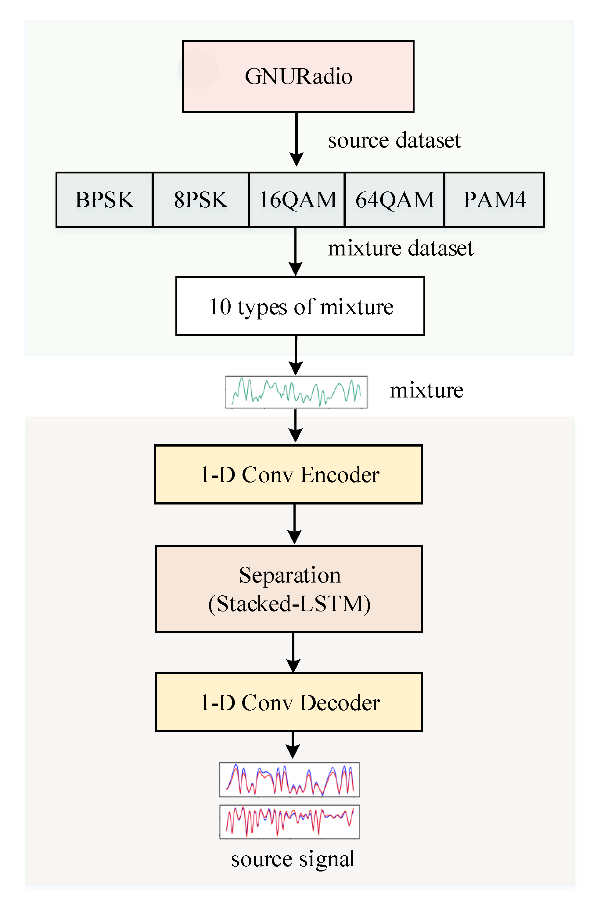
- A mixed communication signal data set 10-mixC is constructed using the GNURadio platform. The data set includes 10 mixed signals obtained from five types of modulation communication signals. This data set can provide data support for similar research work in the future.
- (2)
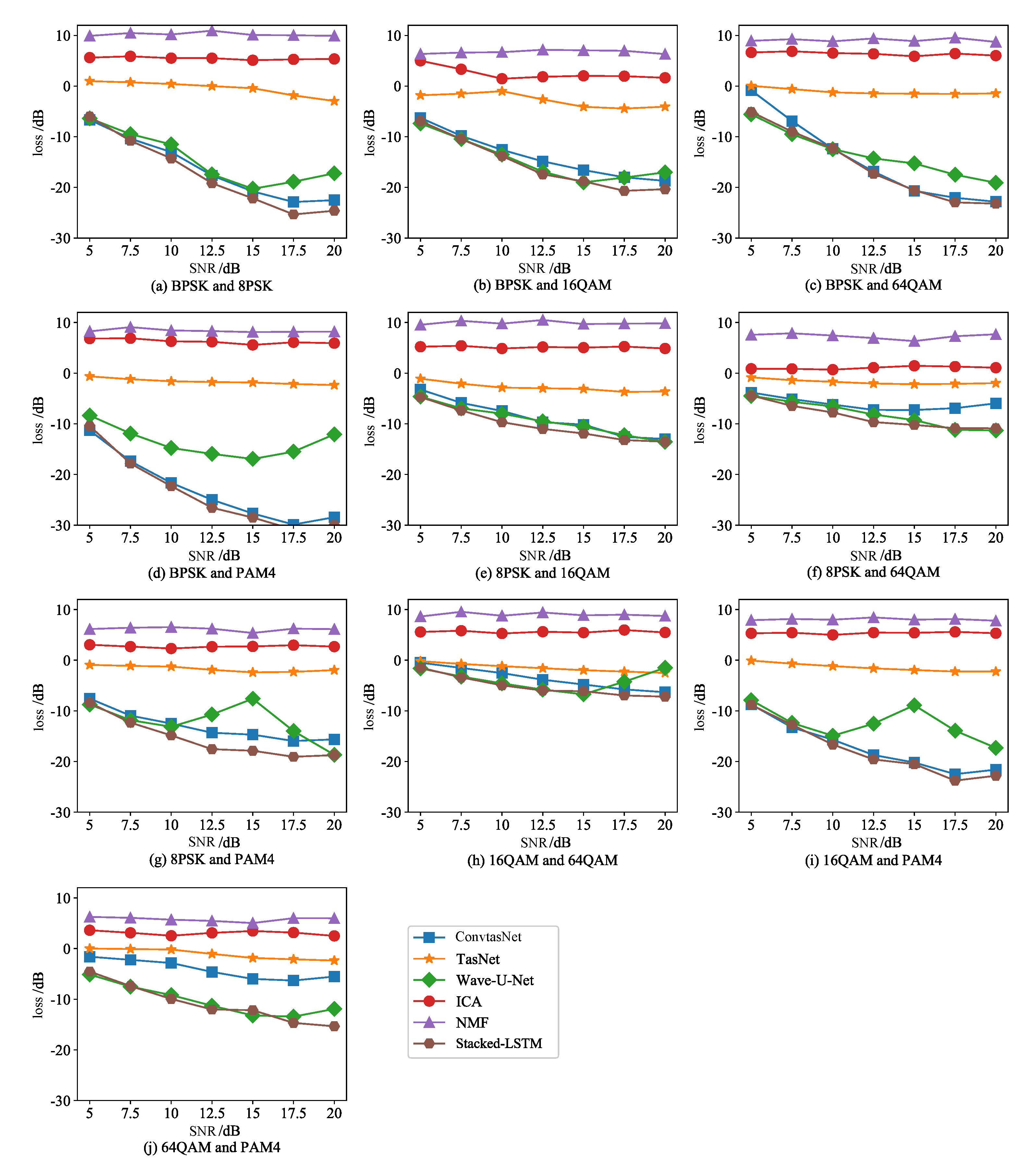
- Stacked-LSTM method improves SISNR by 10.09–38.17 dB compared with the two classic separation algorithms of ICA and NMF and the three deep learning separation methods of TasNet, Conv-TasNet and Wave-U-Net.
- (3)
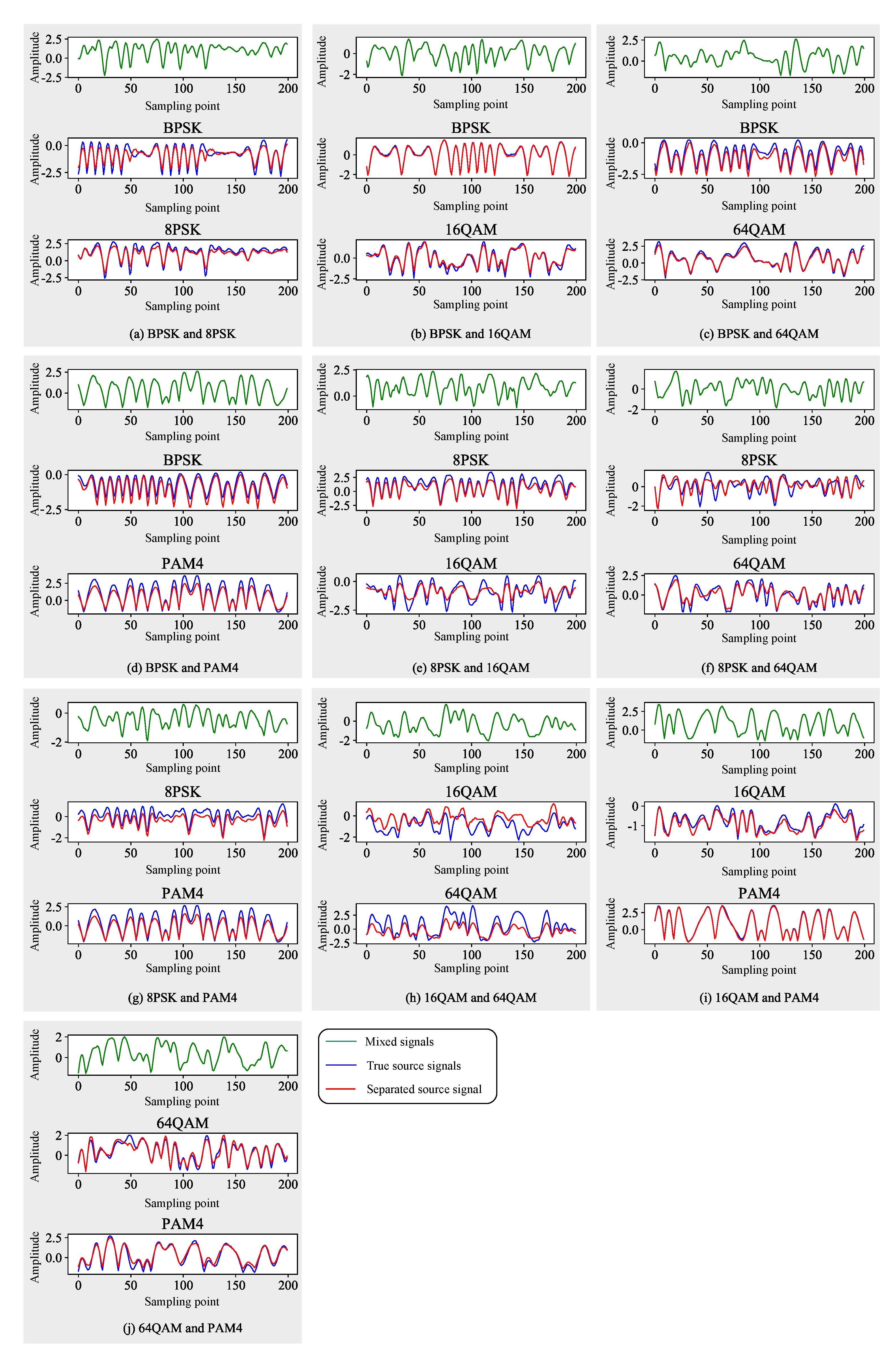
- This method effectively improves the accuracy of blind source separation of single-channel communication signals, and has better noise robustness. It can achieve single-channel separation of 10 mixed signals such as BPSK-16QAM, 8PSK-64QAM, 8PSK-PAM4, 64QAM-PAM4, etc.
2. Related Work
3. Background
3.1. Blind Source Separation
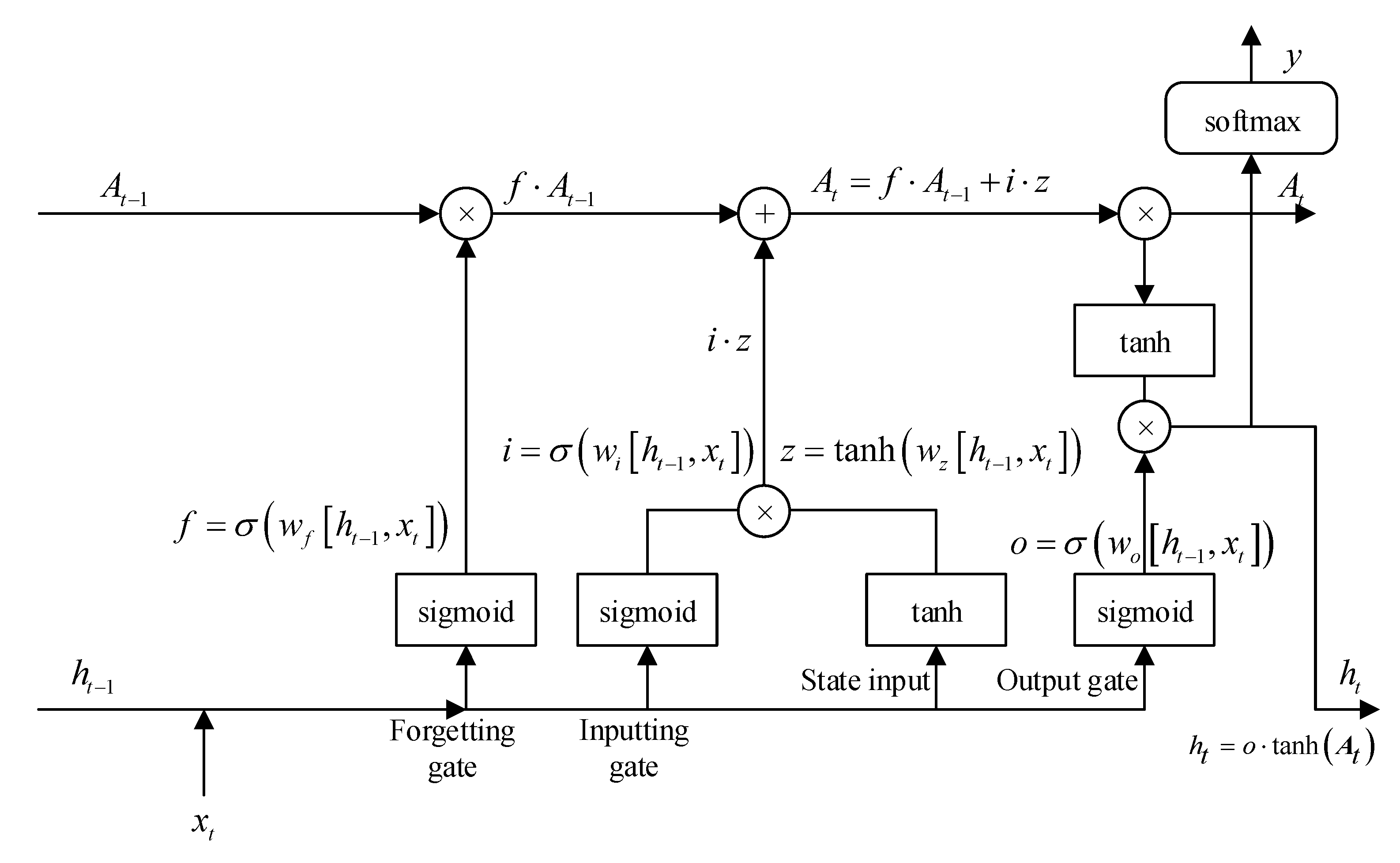
3.2. LSTM
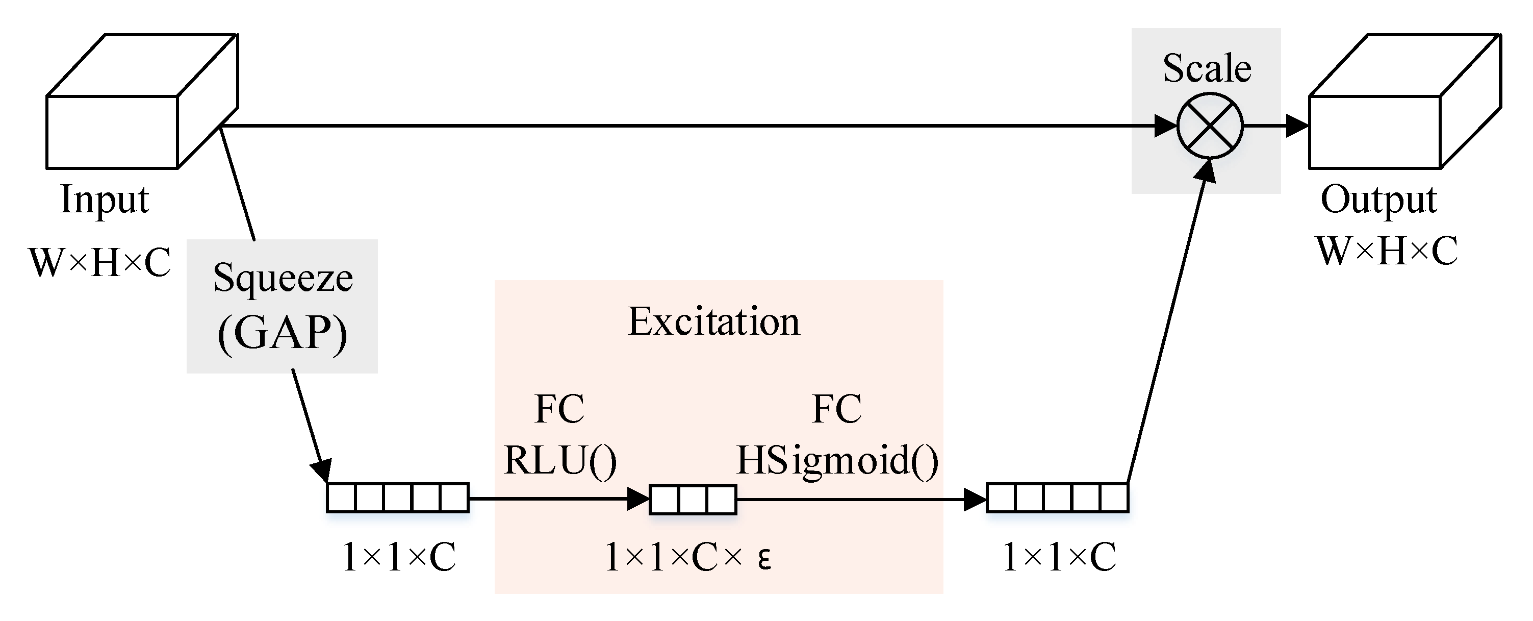
3.3. SE Module
4. Proposed Method
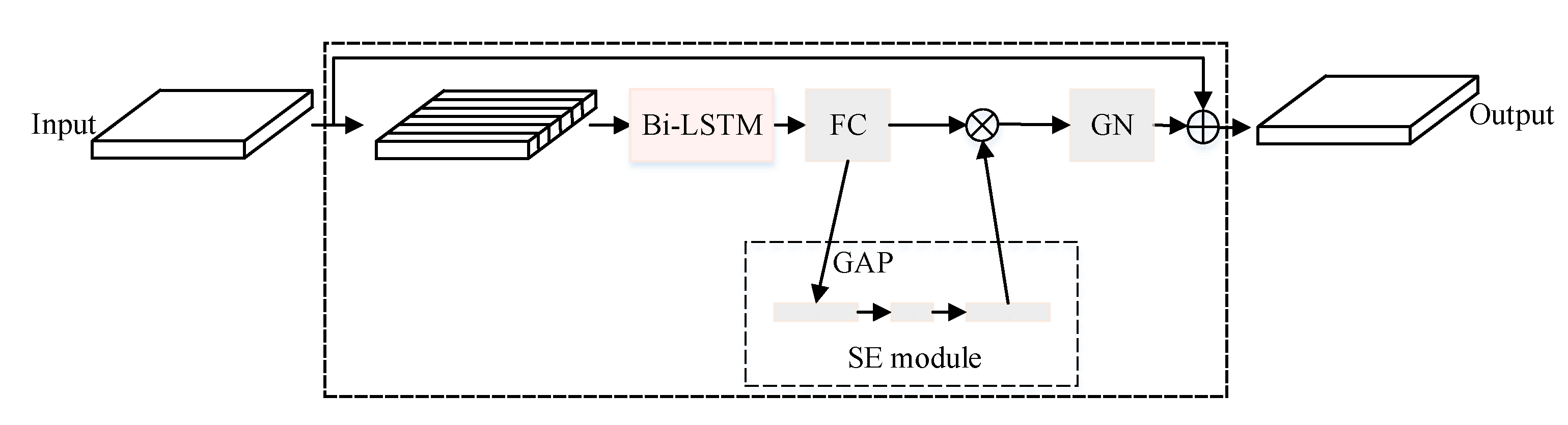
4.1. LSTM Block
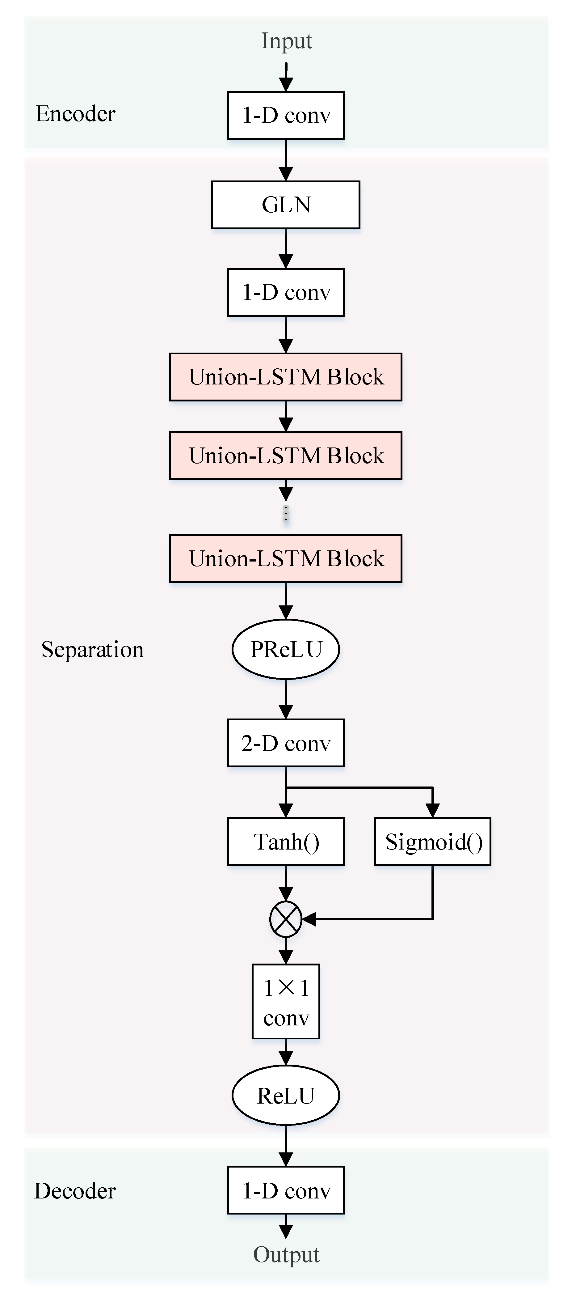
4.2. Stacked-LSTM
4.2.1. Linear Coding of Mixed Signals
4.2.2. Source Signal Mask Generation
4.2.3. Source Signal Waveform Recovery
4.3. Learning Process
5. Experiment
5.1. Dataset
5.2. Experiment Process
5.3. Case Study 1: Effect under Pure Environment
5.4. Case Study 2: Effect under Noisy Environment
5.5. Separation Time Compare
5.6. Application Suggestions
6. Discussion
7. Conclusions
Author Contributions
Funding
Institutional Review Board Statement
Informed Consent Statement
Data Availability Statement
Conflicts of Interest
References
- Shuai, J.; Wang, Z.; Yang, P. Co-frequency signal interference detection based on multiple antennas and multiple channels. J. Phys. Conf. Ser. IOP Publ. 2021, 1738, 012005. [Google Scholar] [CrossRef]
- Jin, F.; Li, Y.; Liu, W.l. Design of Anti-Co-Frequency Interference System for Wireless Spread Spectrum Communication Based on Internet of Things Technology. In Proceedings of the International Conference on Advanced Hybrid Information Processing, Nanjing, China, 21–22 September 2019; pp. 52–61. [Google Scholar]
- Ren, H.; Zheng, Y.; Zhong, N.; Cao, X. Research on Single Antenna Co-frequency Mixed Signal Separation Based on Improved EFICA Algorithm. J. Phys. Conf. Ser. IOP Publ. 2020, 1651, 012052. [Google Scholar] [CrossRef]
- Li, L.; Cai, H.; Han, H.; Jiang, Q.; Ji, H. Adaptive short-time Fourier transform and synchrosqueezing transform for non-stationary signal separation. Signal Process. 2020, 166, 107231. [Google Scholar] [CrossRef]
- Changbo, H.; Lijie, H.; Guowei, L.; Yun, L. Radar signal separation and recognition based on semantic segmentation. In Proceedings of the 2020 7th International Conference on Dependable Systems and Their Applications (DSA), Xi’an, China, 28–29 November 2020; pp. 385–390. [Google Scholar]
- Duong, N.Q.; Vincent, E.; Gribonval, R. Under-determined reverberant audio source separation using a full-rank spatial covariance model. IEEE Trans. Audio Speech Lang. Process. 2010, 18, 1830–1840. [Google Scholar] [CrossRef] [Green Version]
- Lesage, S.; Krstulović, S.; Gribonval, R. Under-determined source separation: Comparison of two approaches based on sparse decompositions. In Proceedings of the International Conference on Independent Component Analysis and Signal Separation, Charleston, SC, USA, 5–8 March 2006; pp. 633–640. [Google Scholar]
- Yang, J.; Guo, Y.; Yang, Z.; Xie, S. Under-determined convolutive blind source separation combining density-based clustering and sparse reconstruction in time-frequency domain. IEEE Trans. Circuits Syst. I Regul. Pap. 2019, 66, 3015–3027. [Google Scholar] [CrossRef]
- Davies, M.E.; James, C.J. Source separation using single channel ICA. Signal Process. 2007, 87, 1819–1832. [Google Scholar] [CrossRef]
- Weninger, F.; Roux, J.L.; Hershey, J.R.; Watanabe, S. Discriminative NMF and its application to single-channel source separation. In Proceedings of the Fifteenth Annual Conference of the International Speech Communication Association, Singapore, 14–18 September 2014. [Google Scholar]
- Luo, Y.; Mesgarani, N. Tasnet: Time-domain audio separation network for real-time, single-channel speech separation. In Proceedings of the 2018 IEEE International Conference on Acoustics, Speech and Signal Processing (ICASSP), Calgary, AB, Canada, 15–20 April 2018; pp. 696–700. [Google Scholar]
- Luo, Y.; Mesgarani, N. Conv-tasnet: Surpassing ideal time—Frequency magnitude masking for speech separation. IEEE/ACM Trans. Audio Speech Lang. Process. 2019, 27, 1256–1266. [Google Scholar] [CrossRef] [Green Version]
- Stoller, D.; Ewert, S.; Dixon, S. Wave-u-net: A multi-scale neural network for end-to-end audio source separation. arXiv 2018, arXiv:1806.03185. [Google Scholar]
- Hu, C.Z.; Yang, Q.; Huang, M.y.; Yan, W.J. Sparse component analysis-based under-determined blind source separation for bearing fault feature extraction in wind turbine gearbox. IET Renew. Power Gener. 2017, 11, 330–337. [Google Scholar] [CrossRef]
- Wang, D.; Chen, J. Supervised Speech Separation Based on Deep Learning: An Overview. IEEE/ACM Trans. Audio Speech Lang. Process. 2018, 26, 1702–1726. [Google Scholar] [CrossRef]
- Lu, X.; Tsao, Y.; Matsuda, S.; Hori, C. Speech enhancement based on deep denoising autoencoder. In Proceedings of the Interspeech, Lyon, France, 25–29 August 2013; Volume 2013, pp. 436–440. [Google Scholar]
- Xu, Y.; Du, J.; Dai, L.R.; Lee, C.H. An experimental study on speech enhancement based on deep neural networks. IEEE Signal Process. Lett. 2013, 21, 65–68. [Google Scholar] [CrossRef]
- Bofill, P.; Zibulevsky, M. Underdetermined blind source separation using sparse representations. Signal Process. 2001, 81, 2353–2362. [Google Scholar] [CrossRef] [Green Version]
- Sadiq, J.S.; Arunmani, G.; Ravivarma, P.; Devi, N.K.; Hemalatha, A.; Ahamed, J.E. Extraction of fetal ECG a semi-blind source separation algorithm combined with parametrized kalman filter. Mater. Today Proc. 2021. [Google Scholar] [CrossRef]
- Jauhar, A.S. A CMA-FRESH Whitening Filter for Blind Interference Rejection. Ph.D. Thesis, Virginia Tech, Blacksburg, VA, USA, 2018. [Google Scholar]
- Yu, L.; Antoni, J.; Wu, H.; Jiang, W. Reconstruction of cyclostationary sound source based on a back-propagating cyclic wiener filter. J. Sound Vib. 2019, 442, 787–799. [Google Scholar] [CrossRef]
- Chollet, F. Xception: Deep learning with depthwise separable convolutions. In Proceedings of the IEEE Conference on Computer Vision and Pattern Recognition, Honolulu, HI, USA, 21–26 July 2017; pp. 1251–1258. [Google Scholar]
- Luo, Y.; Chen, Z.; Yoshioka, T. Dual-path rnn: Efficient long sequence modeling for time-domain single-channel speech separation. In Proceedings of the ICASSP 2020—2020 IEEE International Conference on Acoustics, Speech and Signal Processing (ICASSP), Barcelona, Spain, 4–9 May 2020; pp. 46–50. [Google Scholar]
- Shi, Z.; Liu, R.; Han, J. La furca: Iterative context-aware end-to-end monaural speech separation based on dual-path deep parallel inter-intra bi-lstm with attention. arXiv 2020, arXiv:2001.08998. [Google Scholar]
- Subakan, C.; Ravanelli, M.; Cornell, S.; Bronzi, M.; Zhong, J. Attention is All You Need in Speech Separation. arXiv 2020, arXiv:2010.13154. [Google Scholar]
- Hennequin, R.; Khlif, A.; Voituret, F.; Moussallam, M. Spleeter: A fast and efficient music source separation tool with pre-trained models. J. Open Source Softw. 2020, 5, 2154. [Google Scholar] [CrossRef]
- Han, C.; Luo, Y.; Li, C.; Zhou, T.; Kinoshita, K.; Watanabe, S.; Delcroix, M.; Erdogan, H.; Hershey, J.R.; Mesgarani, N.; et al. Continuous Speech Separation Using Speaker Inventory for Long Multi-talker Recording. arXiv 2020, arXiv:2012.09727. [Google Scholar]
- Fan, C.; Tao, J.; Liu, B.; Yi, J.; Wen, Z.; Liu, X. Deep attention fusion feature for speech separation with end-to-end post-filter method. arXiv 2020, arXiv:2003.07544. [Google Scholar]
- Liu, Y.; Delfarah, M.; Wang, D. Deep CASA for talker-independent monaural speech separation. In Proceedings of the ICASSP 2020—2020 IEEE International Conference on Acoustics, Speech and Signal Processing (ICASSP), Barcelona, Spain, 4–8 May 2020; pp. 6354–6358. [Google Scholar]
- Nguyen, V.N.; Sadeghi, M.; Ricci, E.; Alameda-Pineda, X. Deep Variational Generative Models for Audio-visual Speech Separation. arXiv 2020, arXiv:2008.07191. [Google Scholar]
- Shi, J.; Xu, J.; Fujita, Y.; Watanabe, S.; Xu, B. Speaker-Conditional Chain Model for Speech Separation and Extraction. arXiv 2020, arXiv:2006.14149. [Google Scholar]
- Li, T.; Lin, Q.; Bao, Y.; Li, M. Atss-Net: Target Speaker Separation via Attention-based Neural Network. arXiv 2020, arXiv:2005.09200. [Google Scholar]
- Chang, C.H.; Chung, S.H.; Manthiram, A. Ultra-lightweight PANiNF/MWCNT-functionalized separators with synergistic suppression of polysulfide migration for Li–S batteries with pure sulfur cathodes. J. Mater. Chem. A 2015, 3, 18829–18834. [Google Scholar] [CrossRef]
- Zhang, L.; Shi, Z.; Han, J.; Shi, A.; Ma, D. FurcaNeXt: End-to-End Monaural Speech Separation with Dynamic Gated Dilated Temporal Convolutional Networks. In Proceedings of the International Conference on Multimedia Modeling, Daejeon, Korea, 5–8 January 2020; pp. 653–665. [Google Scholar] [CrossRef]
- Kavalerov, I.; Wisdom, S.; Erdogan, H.; Patton, B.; Wilson, K.; Le Roux, J.; Hershey, J.R. Universal Sound Separation. In Proceedings of the 2019 IEEE Workshop on Applications of Signal Processing to Audio and Acoustics (WASPAA), New Paltz, NY, USA, 20–23 October 2019; pp. 175–179. [Google Scholar] [CrossRef] [Green Version]
- Prétet, L.; Hennequin, R.; Royo-Letelier, J.; Vaglio, A. Singing Voice Separation: A Study on Training Data. In Proceedings of the ICASSP 2019—2019 IEEE International Conference on Acoustics, Speech and Signal Processing (ICASSP), Brighton, UK, 12–17 May 2019; pp. 506–510. [Google Scholar] [CrossRef] [Green Version]
- Luo, Y.; Han, C.; Mesgarani, N.; Ceolini, E.; Liu, S.C. FaSNet: Low-Latency Adaptive Beamforming for Multi-Microphone Audio Processing. In Proceedings of the 2019 IEEE Automatic Speech Recognition and Understanding Workshop (ASRU), Singapore, 14–18 December 2019; pp. 260–267. [Google Scholar] [CrossRef] [Green Version]
- Xu, C.; Wei, R.; Xiao, X.; Chng, E.S.; Li, H. Single Channel Speech Separation with Constrained Utterance Level Permutation Invariant Training Using Grid LSTM. In Proceedings of the ICASSP 2018—2018 IEEE International Conference on Acoustics, Speech and Signal Processing (ICASSP), Calgary, AB, Canada, 15–20 April 2018. [Google Scholar]
- O’Shea, T.J.; Corgan, J.; Clancy, T.C. Convolutional Radio Modulation Recognition Networks. In Engineering Applications of Neural Networks; Jayne, C., Iliadis, L., Eds.; Springer International Publishing: Cham, Switzerland, 2016; pp. 213–226. [Google Scholar]
- Hao, D.D.; Tran, S.T.; Chau, D.T. Speech Separation in the Frequency Domain with Autoencoder. J. Commun. 2020, 15, 841–848. [Google Scholar]
- Gers, F.A.; Schmidhuber, J.; Cummins, F. Learning to Forget: Continual prediction with LSTM. Neural Comput. 2000, 12, 2451–2471. [Google Scholar] [CrossRef] [PubMed]
- Hu, J.; Shen, L.; Sun, G. Squeeze-and-excitation networks. In Proceedings of the IEEE Conference on Computer Vision and Pattern Recognition, Salt Lake City, UT, USA, 18–23 June 2018; pp. 7132–7141. [Google Scholar]
- Li, X.; Wu, J.; Lin, Z.; Liu, H.; Zha, H. Recurrent squeeze-and-excitation context aggregation net for single image deraining. In Proceedings of the European Conference on Computer Vision (ECCV), Munich, Germany, 8–14 September 2018; pp. 254–269. [Google Scholar]
- Li, Y.; Liu, Y.; Cui, W.G.; Guo, Y.Z.; Huang, H.; Hu, Z.Y. Epileptic seizure detection in EEG signals using a unified temporal-spectral squeeze-and-excitation network. IEEE Trans. Neural Syst. Rehabil. Eng. 2020, 28, 782–794. [Google Scholar] [CrossRef]
- Wang, H.; Ji, Z.; Lin, Z.; Pang, Y.; Li, X. Stacked squeeze-and-excitation recurrent residual network for visual-semantic matching. Pattern Recognit. 2020, 105, 107359. [Google Scholar] [CrossRef]
- Chen, J.; Wu, Y.; Yang, Y.; Wen, S.; Shi, K.; Bermak, A.; Huang, T. An efficient memristor-based circuit implementation of squeeze-and-excitation fully convolutional neural networks. IEEE Trans. Neural Networks Learn. Syst. 2021. [Google Scholar] [CrossRef]
- O’Shea, T.J.; Corgan, J.; Clancy, T.C. Convolutional Radio Modulation Recognition Networks; Springer: Cham, Switzerland, 2016. [Google Scholar]
- Khan, Z.Y.; Niu, Z. CNN with depthwise separable convolutions and combined kernels for rating prediction. Expert Syst. Appl. 2021, 170, 114528. [Google Scholar] [CrossRef]
- Isik, Y.; Roux, J.L.; Chen, Z.; Watanabe, S.; Hershey, J.R. Single-Channel Multi-Speaker Separation Using Deep Clustering. arXiv 2016, arXiv:1607.02173. [Google Scholar]
- Fu, W.H.; Wu, S.H.; Liu, N.A.; Yang, B. Underdetermined Blind Source Separation of Frequency Hopping Signal. J. Beijing Univ. Posts Telecommun. 2015, 38, 11. [Google Scholar]
- Zhu, X.; Chang, C.; Yang, L.; Deng, Z.; Cen, X. Time-frequency Aliasing Separation Method of Radar Signal Based on Capsule Neural Network. In Proceedings of the 2020 IEEE 6th International Conference on Computer and Communications (ICCC), Chengdu, China, 11–14 December 2020. [Google Scholar]
- Jia, Y.; Xu, P. Convolutive Blind Source Separation for Communication Signals Based on the Sliding Z-Transform. IEEE Access 2020, 8, 41213–41219. [Google Scholar] [CrossRef]
- Roy, V.; Shukla, S. Designing Efficient Blind Source Separation Methods for EEG Motion Artifact Removal Based on Statistical Evaluation. Wirel. Pers. Commun. 2019, 108, 1311–1327. [Google Scholar] [CrossRef]
- Yu, D.; Kolbk, M.; Tan, Z.H.; Jensen, J. Permutation invariant training of deep models for speaker-independent multi-talker speech separation. In Proceedings of the IEEE International Conference on Acoustics, New Orleans, LA, USA, 5–9 March 2017. [Google Scholar]
- Morten, K.; Yu, D.; Tan, Z.-H.; Jensen, J. Multitalker Speech Separation With Utterance-Level Permutation Invariant Training of Deep Recurrent Neural Networks. IEEE/ACM Trans. Audio, Speech, Lang. Process. 2017, 25, 1901–1913. [Google Scholar]


| Method | Source Signal | SNR (Bb) | Stride (dB) | |
|---|---|---|---|---|
| 1 | BPSK | 5∼30 | 5 | |
| 2 | BPSK, BPSK | 5∼25 | 5 | |
| 3 | QPSK | 12∼22 | 2 | |
| 4 | Radar signal | 10∼30 | 0.5 | |
| 5 | EEG, ECG | / | / | |
| 6 | Speech signal | −6∼9 | 3 | |
| 7 | Speech signal | / | / | |
| 8 | Speech signal | / | / | |
| 9 | Stacked-LSTM | BPSK, 8PSK, 16QAM, 64QAM, PAM4 | 5∼20 | 2.5 |
| Method | Parameter Configuration | Value |
|---|---|---|
| ICA | Iteration number | 100 |
| NMF | Iteration threshold | |
| Iteration number | 100 | |
| TasNet | Base signal number N | 128 |
| Frame length L | 64 | |
| LSTM hidden layer unit number | 128 | |
| LSTM-block number X | 2 | |
| Wave-U-Net | Kernel size P | 5 |
| Block number X | 5 | |
| Channel number | 16-32-64-128-256 | |
| Conv-TasNet | Encoder filter number N | 512 |
| Frame length L | 16 | |
| Bottleneck layer channel number B | 128 | |
| Kernel size P | 3 | |
| 1D-block channel number H | 512 | |
| 1D-block number X | 8 | |
| Repeat number R | 3 | |
| Stacked-LSTM | The number of expected features in the input N | 512 |
| The number of features in th hidden state h | 512 | |
| The number of hidden channels | 256 | |
| Encoder and decoder kernel size P | 16 | |
| Block number X | 6 | |
| The length of chunk K | 200 |
| Mixture | Stacked- LSTM | Conv- TasNet | TasNet | Wave- U-Net | ICA | NMF |
|---|---|---|---|---|---|---|
| BPSK_8PSK | −24.61 | −22.51 | −2.94 | −17.22 | 5.36 | 9.92 |
| BPSK_16QAM | −20.35 | −18.71 | −4.06 | −17.02 | 1.64 | 6.32 |
| BPSK_64QAM | −23.20 | −22.83 | −1.44 | −19.08 | 6.02 | 8.72 |
| BPSK_PAM4 | −29.98 | −28.44 | −2.35 | −12.09 | 5.92 | 8.19 |
| 8PSK_16QAM | −13.53 | −13.00 | −3.63 | −13.55 | 4.87 | 9.82 |
| 8PSK_64QAM | −10.89 | −5.96 | −1.98 | −11.31 | 1.07 | 7.67 |
| 8PSK_PAM4 | −18.74 | −15.64 | −1.95 | −18.67 | 2.68 | 6.13 |
| 16QAM_64QAM | −7.20 | −6.32 | −2.51 | −1.51 | 5.48 | 8.73 |
| 16QAM_PAM4 | −22.81 | −21.61 | −2.25 | −17.31 | 5.32 | 7.79 |
| 64QAM_PAM4 | −15.34 | −5.53 | −2.36 | −11.92 | 2.50 | 5.98 |
| AVG | −18.67 | −16.05 | −2.55 | −13.97 | 4.09 | 7.93 |
| Method | Frame Duration | CPU Computing Time |
|---|---|---|
| Stacked-LSTM time domain mask method | 0.032 | |
| Time-frequency domain mask method | 0.256 | 1.24 |
Publisher’s Note: MDPI stays neutral with regard to jurisdictional claims in published maps and institutional affiliations. |
© 2021 by the authors. Licensee MDPI, Basel, Switzerland. This article is an open access article distributed under the terms and conditions of the Creative Commons Attribution (CC BY) license (https://creativecommons.org/licenses/by/4.0/).
Share and Cite
Zhao, M.; Yao, X.; Wang, J.; Yan, Y.; Gao, X.; Fan, Y. Single-Channel Blind Source Separation of Spatial Aliasing Signal Based on Stacked-LSTM. Sensors 2021, 21, 4844. https://doi.org/10.3390/s21144844
Zhao M, Yao X, Wang J, Yan Y, Gao X, Fan Y. Single-Channel Blind Source Separation of Spatial Aliasing Signal Based on Stacked-LSTM. Sensors. 2021; 21(14):4844. https://doi.org/10.3390/s21144844
Chicago/Turabian StyleZhao, Mengchen, Xiujuan Yao, Jing Wang, Yi Yan, Xiang Gao, and Yanan Fan. 2021. "Single-Channel Blind Source Separation of Spatial Aliasing Signal Based on Stacked-LSTM" Sensors 21, no. 14: 4844. https://doi.org/10.3390/s21144844
APA StyleZhao, M., Yao, X., Wang, J., Yan, Y., Gao, X., & Fan, Y. (2021). Single-Channel Blind Source Separation of Spatial Aliasing Signal Based on Stacked-LSTM. Sensors, 21(14), 4844. https://doi.org/10.3390/s21144844