
Optical Design of Imaging Spectrometer Based on Linear Variable Filter for Nighttime Light Remote Sensing


Abstract
:1. Introduction
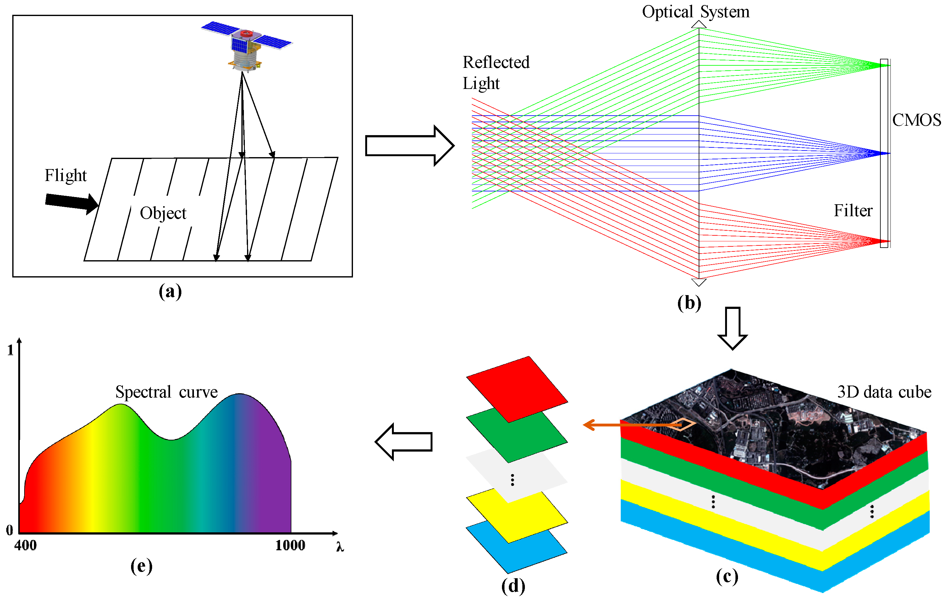
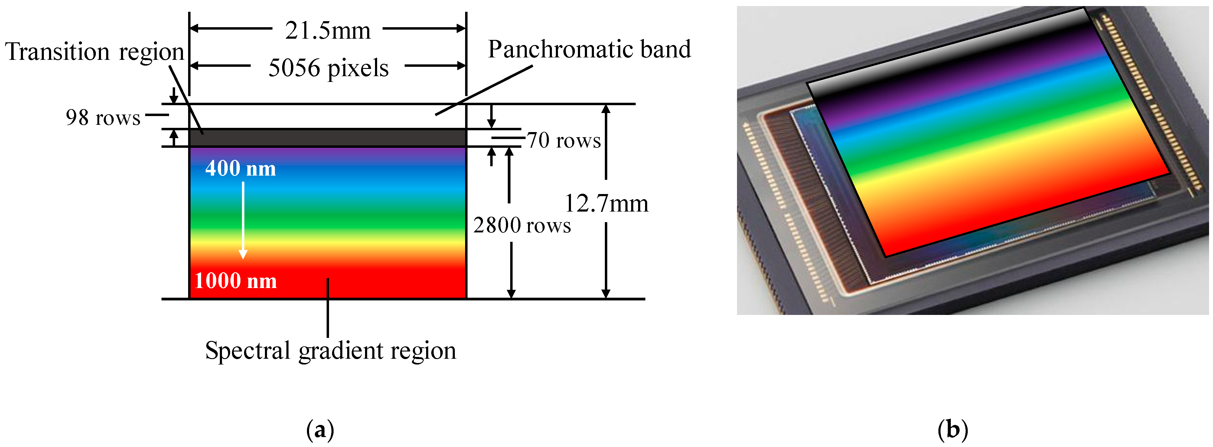
2. Imaging Principle
3. Optical Specifications
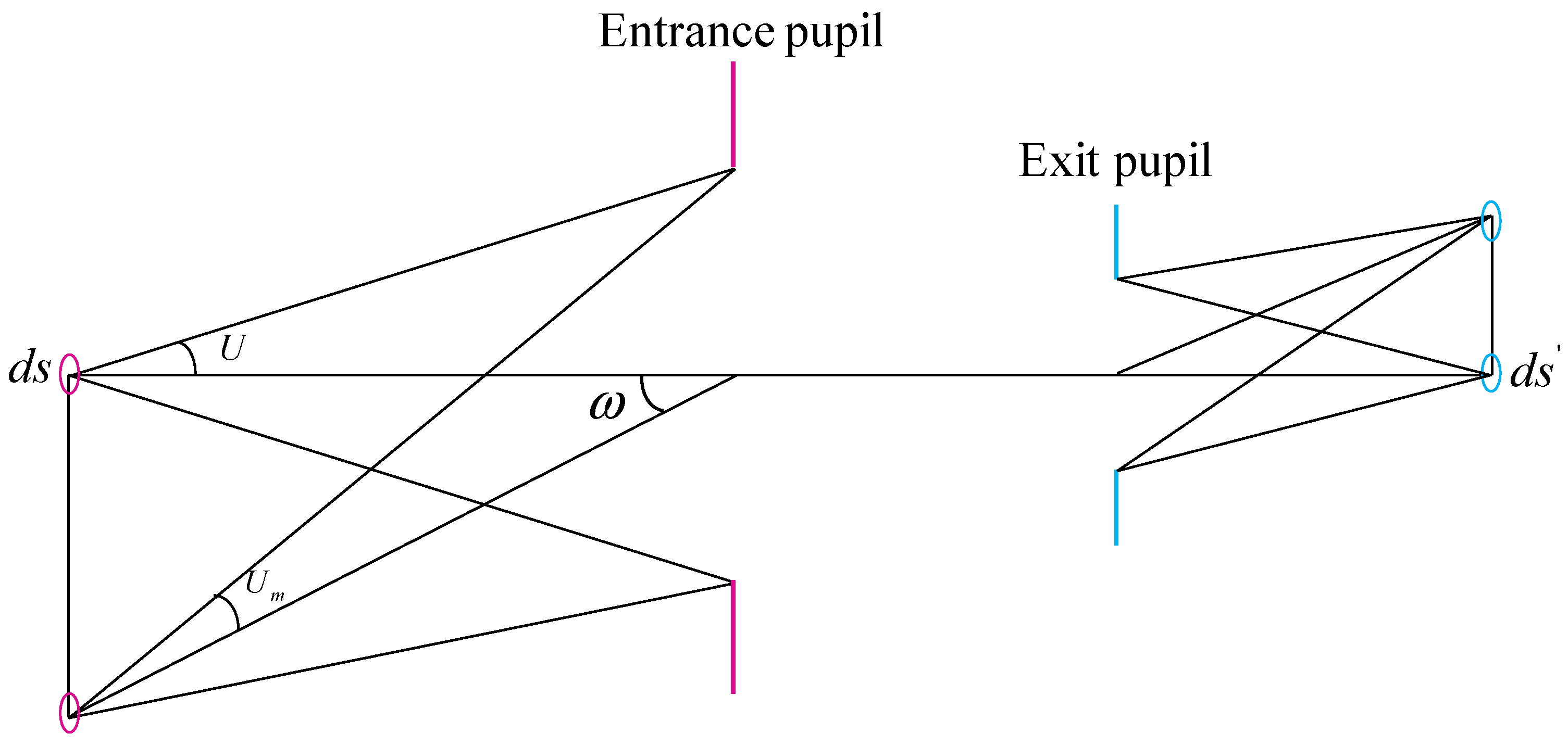
4. Image Plane Illumination Analysis
5. Optical System Design and Optimization
5.1. Initial Optical Structure Design
5.2. Buchdahl Dispersion Model
5.3. Method of Glass Selection for Apochromatic
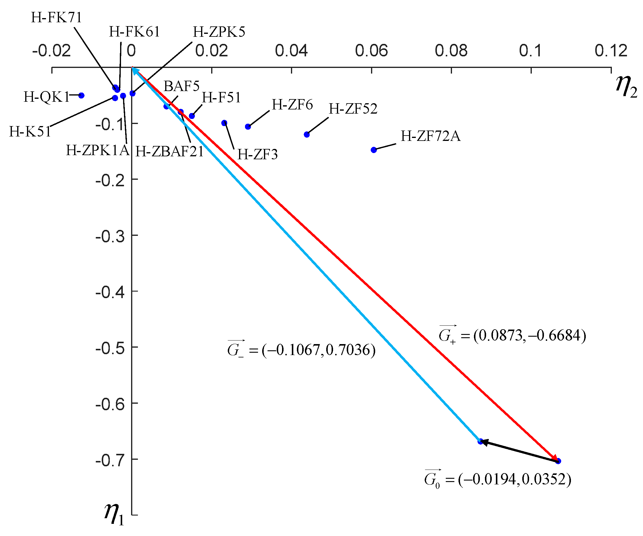
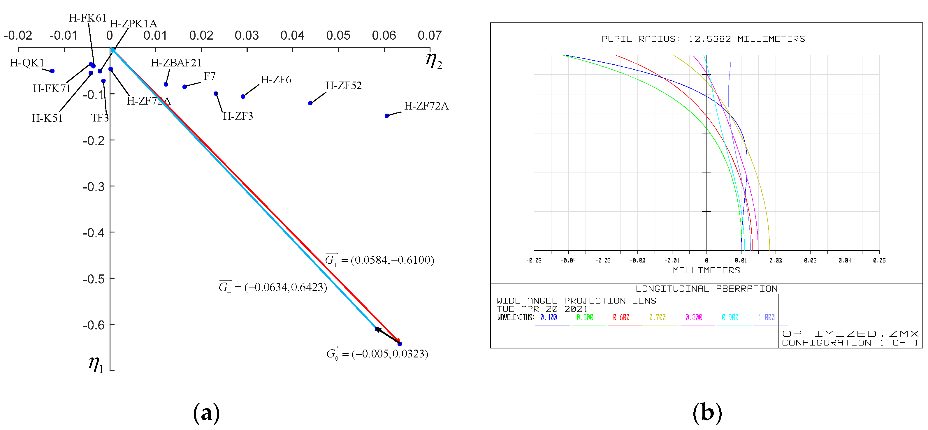
5.4. Dispersion Vector Analysis and Glass Replacement
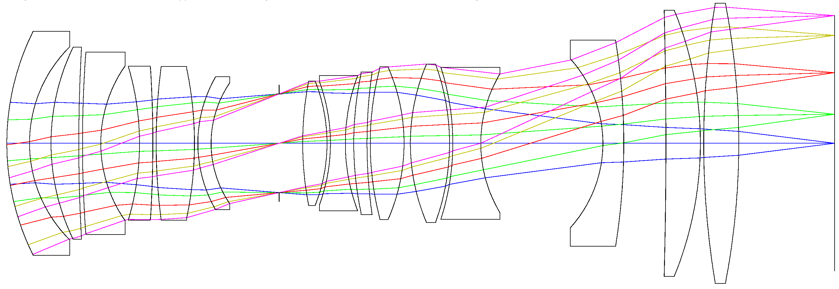
5.5. Final System
6. Image Performance and Tolerance Analysis
6.1. Image Performance
6.2. Tolerance Analysis
7. Discussion and Conclusions
Author Contributions
Funding
Institutional Review Board Statement
Informed Consent Statement
Data Availability Statement
Conflicts of Interest
References
- Levin, N.; Kyba, C.C.M.; Zhang, Q.L.; de Miguel, A.S.; Roman, M.O.; Li, X.; Portnov, B.A.; Molthan, A.L.; Jechow, A.; Miller, S.D.; et al. Remote sensing of nighttime lights: A review and an outlook for the future. Remote Sens. Environ. 2020, 237, 33. [Google Scholar] [CrossRef]
- Levin, N.; Kyba, C.C.M.; Zhang, Q. Remote Sensing of Nighttime lights-Beyond DMSP. Remote Sens. 2019, 11, 1472. [Google Scholar] [CrossRef] [Green Version]
- Li, X.; Elvidge, C.; Zhou, Y.Y.; Cao, C.Y.; Warner, T. Remote sensing of night-time light. Int. J. Remote Sens. 2017, 38, 5855–5859. [Google Scholar] [CrossRef] [Green Version]
- Zheng, Q.M.; Weng, Q.H.; Wang, K. Developing a new cross-sensor calibration model for DMSP-OLS and Suomi-NPP VIIRS night-light imageries. ISPRS J. Photogramm. Remote Sens. 2019, 153, 36–47. [Google Scholar] [CrossRef]
- Li, D.R.; Zhao, X.; Li, X. Remote sensing of human beings—A perspective from nighttime light. Geo-Spat. Inf. Sci. 2016, 19, 69–79. [Google Scholar] [CrossRef] [Green Version]
- Zhao, M.; Zhou, Y.Y.; Li, X.C.; Cao, W.T.; He, C.Y.; Yu, B.L.; Li, X.; Elvidge, C.D.; Cheng, W.M.; Zhou, C.H. Applications of Satellite Remote Sensing of Nighttime Light Observations: Advances, Challenges, and Perspectives. Remote Sens. 2019, 11, 1971. [Google Scholar] [CrossRef] [Green Version]
- Elvidge, C.D.; Imhoff, M.L.; Baugh, K.E.; Hobson, V.R.; Nelson, I.; Safran, J.; Dietz, J.B.; Tuttle, B.T. Night-time lights of the world: 1994–1995. ISPRS J. Photogramm. Remote Sens. 2001, 56, 81–99. [Google Scholar] [CrossRef]
- Elvidge, C.D.; Baugh, K.E.; Zhizhin, M.; Hsu, F.C. Why VIIRS data are superior to DMSP for mapping nighttime lights. Proc. Asia-Pac. Adv. Netw. 2013, 35, 62–69. [Google Scholar] [CrossRef] [Green Version]
- Baugh, K.; Elvidge, C.; Ghosh, T.; Ziskin, D. Development of a 2009 Stable Lights Product using DMSP-OLS data. Proc. Asia-Pac. Adv. Netw. 2010, 30, 114. [Google Scholar] [CrossRef]
- Elvidge, C.D.; Baugh, K.E.; Dietz, J.B.; Bland, T.; Sutton, P.C.; Kroehl, H.W. Radiance calibration of DMSP-OLS low-light imaging data of human settlements. Remote Sens. Environ. 1999, 68, 77–88. [Google Scholar] [CrossRef]
- Miller, S.D.; Straka, W., III; Mills, S.P.; Elvidge, C.D.; Lee, T.F.; Solbrig, J.; Walther, A.; Heidinger, A.K.; Weiss, S.C. Illuminating the Capabilities of the Suomi National Polar-Orbiting Partnership (NPP) Visible Infrared Imaging Radiometer Suite (VIIRS) Day/Night Band. Remote Sens. 2013, 5, 6717–6766. [Google Scholar] [CrossRef] [Green Version]
- Liao, L.B.; Weiss, S.; Mills, S.; Hauss, B. Suomi NPP VIIRS day-night band on-orbit performance. J. Geophys. Res. Atmos. 2013, 118, 12705–12718. [Google Scholar] [CrossRef]
- Liang, C.K.; Mills, S.; Hauss, B.I.; Miller, S.D. Improved VIIRS Day/Night Band Imagery with Near-Constant Contrast. IEEE Trans. Geosci. Remote Sens. 2014, 52, 6964–6971. [Google Scholar] [CrossRef]
- Shi, K.F.; Yu, B.L.; Huang, Y.X.; Hu, Y.J.; Yin, B.; Chen, Z.Q.; Chen, L.J.; Wu, J.P. Evaluating the Ability of NPP-VIIRS Nighttime Light Data to Estimate the Gross Domestic Product and the Electric Power Consumption of China at Multiple Scales: A Comparison with DMSP-OLS Data. Remote Sens. 2014, 6, 1705–1724. [Google Scholar] [CrossRef] [Green Version]
- Small, C.; Elvidge, C.D.; Baugh, K. Mapping Urban Structure and Spatial Connectivity with VIIRS and OLS Nighttime light Imagery. In Proceedings of the Joint Urban Remote Sensing Event 2013, Sao Paulo, Brazil, 21–23 April 2013; pp. 230–233. [Google Scholar] [CrossRef]
- Hillger, D.; Kopp, T.; Lee, T.; Lindsey, D.; Seaman, C.; Miller, S.; Solbrig, J.; Kidder, S.; Bachmeier, S.; Jasmin, T.; et al. First-Light Imagery from Suomi NPP VIIRS. Bull. Amer. Meteorol. Soc. 2013, 94, 1019–1029. [Google Scholar] [CrossRef]
- Li, X.; Zhao, L.X.; Li, D.R.; Xu, H.M. Mapping Urban Extent Using Luojia 1-01 Nighttime Light Imagery. Sensors 2018, 18, 3665. [Google Scholar] [CrossRef] [Green Version]
- Li, X.; Li, X.Y.; Li, D.R.; He, X.J.; Jendryke, M. A preliminary investigation of Luojia-1 night-time light imagery. Remote Sens. Lett. 2019, 10, 526–535. [Google Scholar] [CrossRef]
- Zheng, Q.M.; Weng, Q.H.; Huang, L.Y.; Wang, K.; Deng, J.S.; Jiang, R.W.; Ye, Z.R.; Gan, M.Y. A new source of multi-spectral high spatial resolution night-time light imagery-JL1-3B. Remote Sens. Environ. 2018, 215, 300–312. [Google Scholar] [CrossRef]
- Levin, N.; Johansen, K.; Hacker, J.M.; Phinn, S. A new source for high spatial resolution night time images—The EROS-B commercial satellite. Remote Sens. Environ. 2014, 149, 1–12. [Google Scholar] [CrossRef]
- Kuechly, H.U.; Kyba, C.C.M.; Ruhtz, T.; Lindemann, C.; Wolter, C.; Fischer, J.; Holker, F. Aerial survey and spatial analysis of sources of light pollution in Berlin, Germany. Remote Sens. Environ. 2012, 126, 39–50. [Google Scholar] [CrossRef]
- Elvidge, C.D.; Cinzano, P.; Pettit, D.R.; Arvesen, J.; Sutton, P.; Small, C.; Nemani, R.; Longcore, T.; Rich, C.; Safran, J.; et al. The Nightsat mission concept. Int. J. Remote Sens. 2007, 28, 2645–2670. [Google Scholar] [CrossRef]
- Xue, Q.S.; Tian, Z.T.; Yang, B.; Liang, J.S.; Li, C.; Wang, F.P.; Li, Q. Underwater hyperspectral imaging system using a prism-grating-prism structure. Appl. Opt. 2021, 60, 894–900. [Google Scholar] [CrossRef] [PubMed]
- Chen, J.J.; Yang, J.; Liu, J.N.; Liu, J.L.; Sun, C.; Li, X.T.; Bayanheshig; Cui, J.C. Optics design of a short-wave infrared prism-grating imaging spectrometer. Appl. Opt. 2018, 57, F8–F14. [Google Scholar] [CrossRef]
- Zhu, C.X.; Hobbs, M.J.; Grainger, M.P.; Willmott, J.R. Design and realization of a wide field of view infrared scanning system with an integrated micro-electromechanical system mirror. Appl. Opt. 2018, 57, 10449–10457. [Google Scholar] [CrossRef] [PubMed]
- Chen, L.; Yuan, Q.; Ye, J.F.; Xu, N.Y.; Cao, X.; Gao, Z.S. Design of a compact dual-view endoscope based on a hybrid lens with annularly stitched aspheres. Opt. Commun. 2019, 453, 8. [Google Scholar] [CrossRef]
- Liang, D.; Liang, D.T.; Wang, X.Y.; Li, P. Flexible fluidic lens with polymer membrane and multi-flow structure. Opt. Commun. 2018, 421, 7–13. [Google Scholar] [CrossRef]
- Grammatin, A.P.; Kolesnik, E.V. Calculations for optical systems, using the method of simulation modelling. J. Opt. Technol. 2004, 71, 211–213. [Google Scholar] [CrossRef]
- Sigler, R.D. Apochromatic color correction using liquid lenses. Appl. Opt. 1990, 29, 2451–2459. [Google Scholar] [CrossRef] [PubMed]
- Sigler, R.D. Glass selection for airspaced apochromats using the Buchdal dispersion equation. Appl. Opt. 1986, 25, 4311–4320. [Google Scholar] [CrossRef]
- Pawlowski, M.E.; Dwight, J.G.; Thuc Uyen, N.; Tkaczyk, T.S. High performance image mapping spectrometer (IMS) for snapshot hyperspectral imaging applications. Opt. Express 2019, 27, 1597–1612. [Google Scholar] [CrossRef]
- Fotios, S.; Gibbons, R. Road lighting research for drivers and pedestrians: The basis of luminance and illuminance recommendations. Lighting Res. Technol. 2018, 50, 154–186. [Google Scholar] [CrossRef]
- Kyba, C.C.M.; Garz, S.; Kuechly, H.; de Miguel, A.S.; Zamorano, J.; Fischer, J.; Holker, F. High-Resolution Imagery of Earth at Night: New Sources, Opportunities and Challenges. Remote Sens. 2015, 7, 1–23. [Google Scholar] [CrossRef] [Green Version]
- Gpixel. Available online: https://www.gpixel.com/ (accessed on 10 June 2021).
- De Meester, J.; Storch, T. Optimized Performance Parameters for Nighttime Multispectral Satellite Imagery to Analyze Lightings in Urban Areas. Sensors 2020, 20, 3313. [Google Scholar] [CrossRef] [PubMed]
- Yao, Y.; Xu, Y.; Ding, Y.; Yuan, G. Optical-system design for large field-of-view three-line array airborne mapping camera. Opt. Precis. Eng. 2018, 26, 2334–2343. [Google Scholar] [CrossRef]
- Zhang, Z.D.; Zheng, W.B.; Gong, D.; Li, H.Z. Design of a zoom telescope optical system with a large aperture, long focal length, and wide field of view via a catadioptric switching solution. J. Opt. Technol. 2021, 88, 14–20. [Google Scholar] [CrossRef]
- Shi, Z.; Yu, L.; Cao, D.; Wu, Q.; Yu, X.; Lin, G. Airborne ultraviolet imaging system for oil slick surveillance: Oil-seawater contrast, imaging concept, signal-to-noise ratio, optical design, and optomechanical model. Appl. Opt. 2015, 54, 7648–7655. [Google Scholar] [CrossRef]
- Mouroulis, P.; Macdonald, J. Geometrical Optics and Optical Design; Oxford University Press: Oxford, UK, 1997. [Google Scholar]
- Reshidko, D.; Sasian, J. Role of aberrations in the relative illumination of a lens system. Opt. Eng. 2016, 55, 12. [Google Scholar] [CrossRef] [Green Version]
- Johnson, T.P.; Sasian, J. Image distortion, pupil coma, and relative illumination. Appl. Opt. 2020, 59, G19–G23. [Google Scholar] [CrossRef]
- Robb, P.N.; Mercado, R.I. Calculation of refractive indices using Buchdahl’s chromatic coordinate. Appl. Opt. 1983, 22, 1198–1215. [Google Scholar] [CrossRef]
- Reardon, P.J.; Chipman, R.A. Buchdahl’s glass dispersion coefficients calculated from Schott equation constants. Appl. Opt. 1989, 28, 3520–3523. [Google Scholar] [CrossRef]
- Chipman, R.A.; Reardon, P.J. Buchdahl’s glass dispersion coefficients calculated in the near-infrared. Appl. Opt. 1989, 28, 694–698. [Google Scholar] [CrossRef] [PubMed]
- Wang, W.; Zhong, X.; Liu, J.; Wang, X.H. Apochromatic lens design in he short-wave infrared band using the Buchdahl dispersion mode. Appl. Opt. 2019, 58, 892–903. [Google Scholar] [CrossRef] [PubMed]


| Parameters | Value |
|---|---|
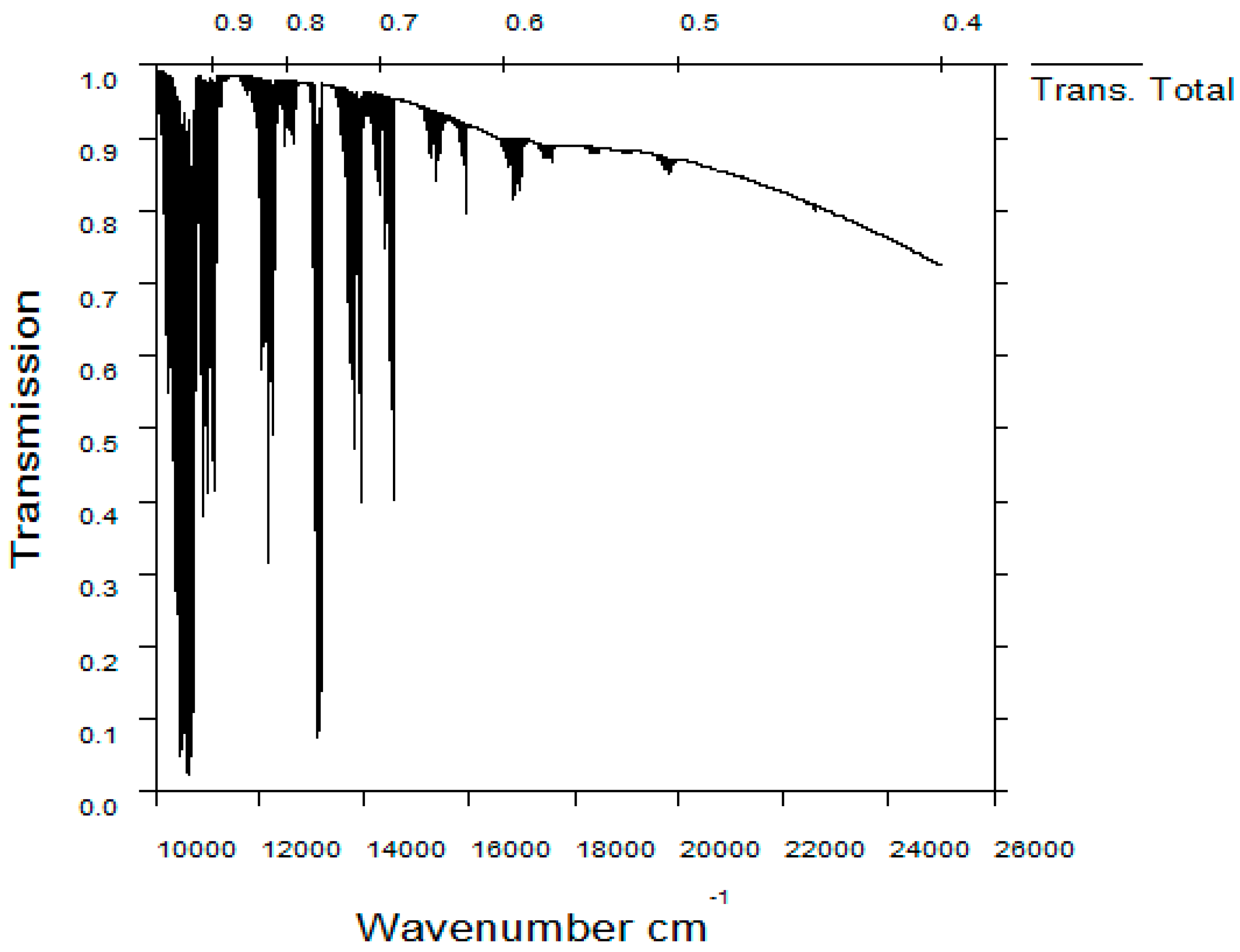
| Model Atmosphere | Middle altitude summer |
| Water vapor column | 1.0 gm/cm2 |
| CO2 Mixing Ratio | 330.0 ppmv |
| Aerosol model used | Rural –VIS-23km |
| Parameters | Value |
|---|---|
| Wavelength range | 400–1000 nm |
| Focal length | 100 mm |
| F-number | 4 |
| Field of view | ±21.5° |
| MTF | >0.3@118lp/mm |
| Distortion | <0.05% |
| 1 | 2 | 3 | 4 | 5 | 6 | 7 | ||
| Glass | H-K51 | H-ZF3 | H-FK71 | H-ZF6 | H-ZBAF21 | H-ZF6 | H-ZPK1A | |
| −0.006834 | 0.01047 | −0.00721 | −0.008528 | 0.009377 | −0.006079 | 0.0192 | ||
| 12.539 | 12.636 | 11.958 | 11.936 | 13.251 | 14.274 | 14.412 | ||
| 1.5190 | 1.7069 | 1.4542 | 1.7435 | 1.7151 | 1.7435 | 1.6135 | ||
| −0.6856 | 1.0666 | −0.6578 | −0.7752 | 1.0505 | −0.7902 | 2.5444 | ||
| −0.0549 | −0.0995 | −0.0362 | −0.1060 | −0.0797 | −0.1060 | −0.0509 | ||
| −0.0042 | 0.0232 | −0.0041 | 0.0291 | 0.0122 | 0.0291 | −0.0022 | ||
| 8 | 9 | 10 | 11 | 12 | 13 | 14 | 15 | |
| Glass | BAF5 | H-ZF72A | H-FK61 | H-ZPK5 | H-F51 | H-QK1 | H-ZF52 | H-ZBAF21 |
| −0.02546 | 0.006623 | 0.01426 | 0.0188 | −0.02664 | −0.009781 | 0.009608 | 0.004847 | |
| 14.252 | 14.664 | 14.754 | 14.298 | 12.628 | 5.836 | 4.816 | 4.321 | |
| 1.5995 | 1.9027 | 1.4942 | 1.5889 | 1.6317 | 1.4672 | 1.8316 | 1.7151 | |
| −3.2995 | 0.9087 | 1.9805 | 2.4522 | −2.7105 | −0.2125 | 0.1422 | 0.0577 | |
| −0.0697 | −0.1476 | −0.04 | −0.0465 | −0.0869 | −0.0504 | −0.1201 | −0.0797 | |
| 0.0087 | 0.0606 | −0.0036 | 0.00017124 | 0.0150 | −0.0126 | 0.0438 | 0.0122 | |
| 1 | 2 | 3 | 4 | 5 | 6 | 7 | ||
| Glass | H-K51 | H-ZF3 | H-FK71 | H-ZF6 | H-ZBAF21 | H-ZF6 | H-ZPK1A | |
| −0.005773 | 0.009655 | −0.008114 | −0.008616 | 0.01 | −0.003131 | 0.018 | ||
| 12.637 | 12.660 | 12.289 | 12.447 | 13.773 | 14.137 | 15.779 | ||
| 1.5190 | 1.7069 | 1.4542 | 1.7435 | 1.7151 | 1.7435 | 1.6135 | ||
| −0.5836 | 0.9796 | −0.7757 | −0.8450 | 1.2009 | −0.3961 | 2.8370 | ||
| −0.0549 | −0.0995 | −0.0362 | −0.1060 | −0.0797 | −0.1060 | −0.0509 | ||
| −0.0042 | 0.0232 | −0.0041 | 0.0291 | 0.0122 | 0.0291 | −0.0022 | ||
| 8 | 9 | 10 | 11 | 12 | 13 | 14 | 15 | |
| Glass | TF3 | H-ZF72A | H-FK61 | H-ZPK5 | F7 | H-QK1 | H-ZF52 | H-ZBAF21 |
| −0.021 | 0.003113 | 0.013 | 0.016 | −0.023 | −0.009421 | 0.007063 | 0.005341 | |
| Yj | 15.490 | 15.556 | 15.581 | 14.938 | 13.025 | 6.211 | 4.738 | 4.298 |
| N0 | 1.6062 | 1.9027 | 1.4942 | 1.5889 | 1.6285 | 1.4672 | 1.8316 | 1.7151 |
| −3.1897 | 0.4769 | 1.9979 | 2.2602 | −2.4701 | −0.2301 | 0.1004 | 0.0625 | |
| −0.0719 | −0.1476 | −0.04 | −0.0465 | −0.0849 | −0.0504 | −0.1201 | −0.0797 | |
| −0.0014 | 0.0606 | −0.0036 | 0.00017124 | 0.0163 | −0.0126 | 0.0438 | 0.0122 | |
| Tolerance Items | Value |
|---|---|
| Radius (fringes) | 1 |
| Thickness (mm) | 0.01 |
| Decenter X/Y (mm) | 0.01 |
| Tilt X/Y (degrees) | 0.0042 |
| S + A irregularity (fringes) | 0.2 |
| Index of refraction | 0.0003 |
| Abbe number (%) | 0.5 |
Publisher’s Note: MDPI stays neutral with regard to jurisdictional claims in published maps and institutional affiliations. |
© 2021 by the authors. Licensee MDPI, Basel, Switzerland. This article is an open access article distributed under the terms and conditions of the Creative Commons Attribution (CC BY) license (https://creativecommons.org/licenses/by/4.0/).
Share and Cite
Xie, Y.; Liu, C.; Liu, S.; Fan, X. Optical Design of Imaging Spectrometer Based on Linear Variable Filter for Nighttime Light Remote Sensing. Sensors 2021, 21, 4313. https://doi.org/10.3390/s21134313
Xie Y, Liu C, Liu S, Fan X. Optical Design of Imaging Spectrometer Based on Linear Variable Filter for Nighttime Light Remote Sensing. Sensors. 2021; 21(13):4313. https://doi.org/10.3390/s21134313
Chicago/Turabian StyleXie, Yunqiang, Chunyu Liu, Shuai Liu, and Xinghao Fan. 2021. "Optical Design of Imaging Spectrometer Based on Linear Variable Filter for Nighttime Light Remote Sensing" Sensors 21, no. 13: 4313. https://doi.org/10.3390/s21134313
APA StyleXie, Y., Liu, C., Liu, S., & Fan, X. (2021). Optical Design of Imaging Spectrometer Based on Linear Variable Filter for Nighttime Light Remote Sensing. Sensors, 21(13), 4313. https://doi.org/10.3390/s21134313