
The Deep Learning Solutions on Lossless Compression Methods for Alleviating Data Load on IoT Nodes in Smart Cities


Abstract
1. Introduction
- (1)
- We study the technical side of IoT memory to clarify why small IoT memory cannot handle massive amounts of data.
- (2)
- We investigate lossless compression algorithms as well as previous and current related work that has been used to reduce data size and illustrated detailed differences between them to clarify which can be used for IoT.
- (3)
- We demonstrate the fundamentals of deep learning, which later help us understand the techniques used for dimension reduction and how we can use them to compress data in IoT memory.
- (4)
- We implement experiments on five datasets using lossless compression algorithms to justify which fits better for IoT and which is more suitable for numeric and time series data type as IoT data type.
2. Internet of Things
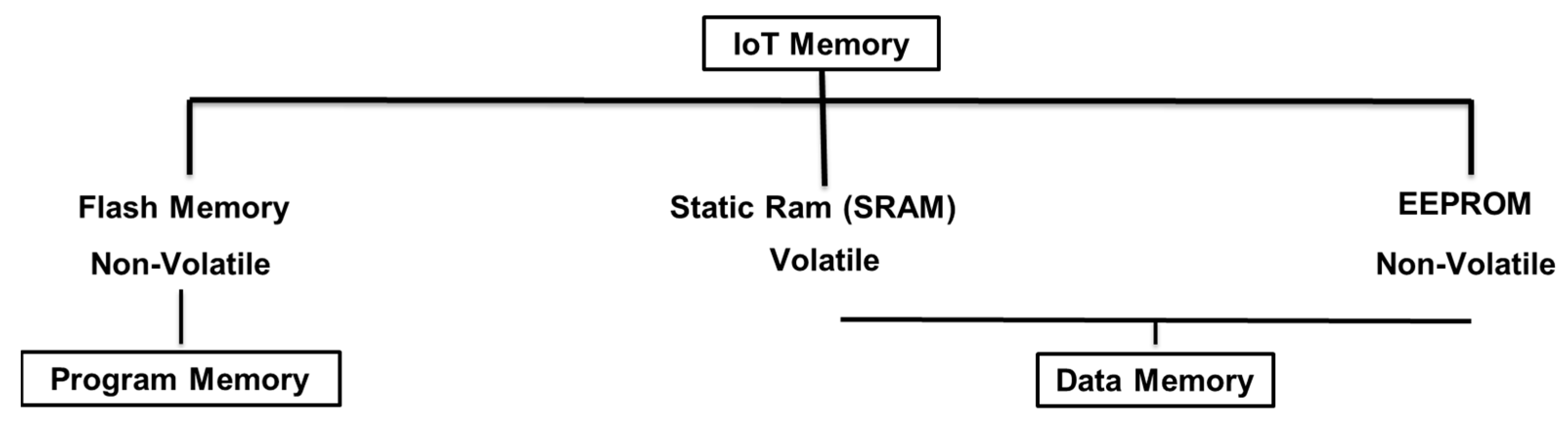
2.1. IoT Memory
2.2. The IoT Memory Challenge
2.3. The IoT Data Traffic Reduction Motivations
2.4. The IoT Data Compression State of Art
3. Compression
3.1. Lossless Data Compression
3.1.1. Lossless Entropy Algorithms
3.1.2. Lossless Dictionary Based Algorithms
3.1.3. Lossless General Compression Algorithms
4. Deep Learning
4.1. Deep Learning Architectures
4.2. Dimensionality Reduction Techniques
4.2.1. Pruning
4.2.2. Pooling
5. Deep Learning Solutions for IoT Data Compression
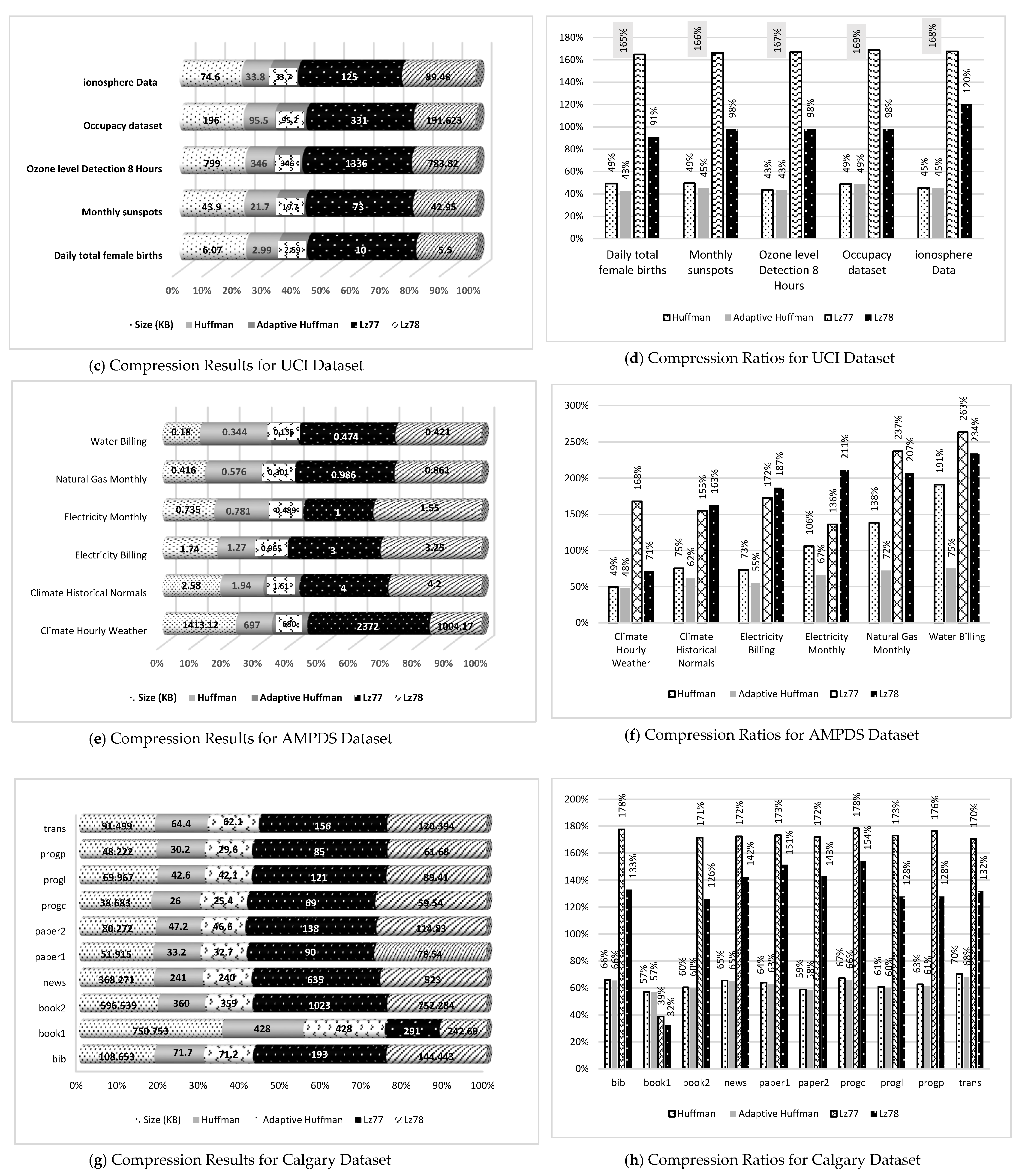
6. Experiments and Results
- (1)
- The first type is a time-series dataset collected from sensors connected to IoT devices,
- (2)
- The second type is time-series data not collected by sensors or IoT devices, and
- (3)
- The third type is a collection of varied files, not time series, and not collected by sensors or IoT devices.
7. Discussion
8. Conclusions, Challenges and Future Work
Author Contributions
Funding
Institutional Review Board Statement
Informed Consent Statement
Data Availability Statement
Conflicts of Interest
References
- Siyuan, C. World Urbanization Prospects. In Proceedings of the United Nations, Department of Economic and Social Affairs; United Nations: New York, NY, USA, 2014; Volume 1, pp. 1–32. [Google Scholar]
- Eremia, M.; Toma, L.; Sanduleac, M. The Smart City Concept in the 21st Century. Procedia Eng. 2017, 181, 12–19. [Google Scholar] [CrossRef]
- Hoornweg, D.; Pope, K. Socioeconomic Pathways and Regional Distribution of the World’s 101 Largest Cities; Global Cities Institute: Oshawa, ON, Canada, 2014; Volume 1. [Google Scholar]
- Bajer, M. Building an IoT data hub with elasticsearch, Logstash and Kibana. In Proceedings of the 2017 5th International Conference on Future Internet of Things and Cloud Workshops (FiCloudW), Prague, Czech Republic, 21–23 August 2017; pp. 63–68. [Google Scholar] [CrossRef]
- Schuler, D. Digital Cities and Digital Citizens; Springer: Berlin/Heidelberg, Germany, 2002; pp. 71–85. [Google Scholar]
- Deren, L.; Qing, Z.; Xiafei, L. Cybercity: Conception, technical supports and typical applications. Geo-Spat. Inf. Sci. 2000, 3, 1–8. [Google Scholar] [CrossRef][Green Version]
- Ishida, T.; Isbister, K. Digital Cities: Technologies, Experiences, and Future Perspectives—Google Books; Springer Science & Business Media: Berlin, Germany, 2000; ISBN 0302-9743. [Google Scholar]
- Komninos, N. Intelligent Cities and Globalisation of Innovation Networks; Routledge: London, UK, 2008; ISBN 0203894499. [Google Scholar]
- Shepard, M. Sentient City: Ubiquitous Computing, Architecture, and the Future of Urban Space, 1st ed.; Shepard, M., Ed.; Architectural League of New York, The MIT Press: New York, NY, USA, 2011; ISBN 9780262515863. [Google Scholar]
- Bătăgan, L. la psicología de la salud en el nuevo currículo de la diplomatura en enfermería. Rev. Enfermer 2011, 18, 80–87. [Google Scholar]
- Jedliński, M. The Position of Green Logistics in Sustainable Development of a Smart Green City. Procedia Soc. Behav. Sci. 2014, 151, 102–111. [Google Scholar] [CrossRef]
- Heiner, M.; Gilbert, D.; Donaldson, R. Petri nets for systems and synthetic biology. Lect. Notes Comput. Sci. (Subser. Lect. Notes Artif. Intell. Lect. Notes Bioinform.) 2008, 5016 LNCS, 215–264. [Google Scholar] [CrossRef]
- Kang, J.; Eom, D.S. Offloading and transmission strategies for IoT edge devices and networks. Sensors 2019, 19, 835. [Google Scholar] [CrossRef] [PubMed]
- Vanolo, A. Smartmentality: The Smart City as Disciplinary Strategy. Urban Stud. 2014, 51, 883–898. [Google Scholar] [CrossRef]
- Lea, R.; Blackstock, M. Smart Cities: An IoT-centric Approach. In Proceedings of the 2014 International Workshop on Web Intelligence and Smart Sensing, New York, NY, USA, 1–2 September 2014; International Workshop on Web Intelligence and Smart Sensing, Association for Computing Machinery: New York, NY, USA, 2014. [Google Scholar] [CrossRef]
- Kim, J.S. Reviewed paper Mapping Conflicts in the Development of Smart Cities: The Experience of Using Q Methodology for Smart Gusu Project, Suzhou, China Joon Sik Kim. In Proceedings of the 21st International Conference on Urban Planning, Regional Development and Information Society, Hamburg, Germany, 22–24 June 2016; Volume 2, pp. 437–446. [Google Scholar]
- Park, E.; P, A.; Pobil, D.; Jib Kwon, S. The role of the Internet of Things in developing smart cities. Sustainability 2018, 14, 1388. [Google Scholar] [CrossRef]
- Lauriault, T.P.; Bloom, R.; Livingstone, C.; Landry, J.-N. Open Smart Cities in Canada: Environmental Scan and Case Studies. OpenNorth 2018, 33. [Google Scholar] [CrossRef]
- Abusaada, H.; Elshater, A. Competitiveness, distinctiveness and singularity in urban design: A systematic review and framework for smart cities. Sustain. Cities Soc. 2021, 68, 102782. [Google Scholar] [CrossRef]
- Nevado Gil, M.T.; Carvalho, L.; Paiva, I. Determining factors in becoming a sustainable smart city: An empirical study in Europe. Econ. Sociol. 2020, 13, 24–39. [Google Scholar] [CrossRef]
- Lipman Jim NVM Memory: A Critical Design Consideration for IoT Applications. Available online: https://www.design-reuse.com/articles/32614/nvm-memory-iot-applications.html (accessed on 16 February 2019).
- Chourabi, H.; Nam, T.; Walker, S.; Gil-Garcia, J.R.; Mellouli, S.; Nahon, K.; Pardo, T.A.; Scholl, H.J. Understanding smart cities: An integrative framework. In Proceedings of the 2012 45th Hawaii International Conference on System Sciences, Maui, HI, USA, 4–7 January 2012; pp. 2289–2297. [Google Scholar] [CrossRef]
- Teuben, H.; Dijik, V. Smart Cities. Netherlands. 2015. Available online: https://www2.deloitte.com/content/dam/Deloitte/tr/Documents/public-sector/deloitte-nl-ps-smart-cities-report.pdf (accessed on 18 May 2021).
- Pham, C. Tokyo Smart City Development in Perspective of 2020 Olympics Opportunities for EU-Japan Cooperation and Business Development. Available online: https://www.eu-japan.eu/sites/default/files/publications/docs/smart2020tokyo_final.pdf (accessed on 18 May 2021).
- Madox, T. Teena Maddox|US|Meet the Team—TechRepublic. Available online: https://www.techrepublic.com/meet-the-team/us/teena-maddox/ (accessed on 22 November 2018).
- Alenezi, A. Challenges of IoT Based Smart City Development in Kuwait. Ph.D. Thesis, Kuwait University, Kuwait City, Kuwait, 2017. [Google Scholar] [CrossRef]
- Trilles, S.; Calia, A.; Belmonte, Ó.; Torres-Sospedra, J.; Montoliu, R.; Huerta, J. Deployment of an open sensorized platform in a smart city context. Futur. Gener. Comput. Syst. 2017, 76, 221–233. [Google Scholar] [CrossRef]
- Goodspeed, R. Smart cities: Moving beyond urban cybernetics to tackle wicked problems. Camb. J. Reg. Econ. Soc. 2015, 8, 79–92. [Google Scholar] [CrossRef]
- Moustaka, V.; Vakali, A. Smart Cities at Risk! Privacy and Security Borderlines from Social Networking in Cities. In Proceedings of the Companion Proceedings of the The Web Conference 2018, Lyon, France, 23–27 April 2018; pp. 905–910. [Google Scholar] [CrossRef]
- Rana, N.P.; Luthra, S.; Mangla, S.K.; Islam, R.; Roderick, S.; Dwivedi, Y.K. Barriers to the Development of Smart Cities in Indian Context. Inf. Syst. Front. 2019, 21, 503–525. [Google Scholar] [CrossRef]
- Lee, G.M.; Kim, J.Y. The Internet of Things—A problem statement. In Proceedings of the 2010 International Conference on Information and Communication Technology Convergence (ICTC), Jeju, Korea, 17–19 November 2010; pp. 517–518. [Google Scholar] [CrossRef]
- Tareq, M.; Sundararajan, E.A.; Mohd, M.; Sani, N.S. Online clustering of evolving data streams using a density grid-based method. IEEE Access 2020, 8, 166472–166490. [Google Scholar] [CrossRef]
- Verhelst, M.; Moons, B. Embedded Deep Neural Network Processing: Algorithmic and Processor Techniques Bring Deep Learning to IoT and Edge Devices. IEEE Solid-State Circuits Mag. 2017, 9, 55–65. [Google Scholar] [CrossRef]
- Kim, T.; Ramos, C.; Mohammed, S. Smart City and IoT. Futur. Gener. Comput. Syst. 2017, 76, 159–162. [Google Scholar] [CrossRef]
- Li, H.; Ota, K.; Dong, M. Learning IoT in Edge: Deep Learning for the Internet of Things with Edge Computing. IEEE Netw. 2018, 32, 96–101. [Google Scholar] [CrossRef]
- Stojkoska, B.R.; Nikolovski, Z. Data compression for energy efficient IoT solutions. In Proceedings of the 25th Telecommunication Forum (TELFOR), Belgrade, Serbia, 21–22 November 2017. [Google Scholar] [CrossRef]
- Akhtar, N.; Hasley, K. Smart Cities Face Challenges and Opportunities. Available online: https://www.computerweekly.com/opinion/Smart-cities-face-challenges-and-opportunities (accessed on 24 November 2018).
- Liu, J.; Chen, F.; Wang, D. Data compression based on stacked RBM-AE model for wireless sensor networks. Sensors 2018, 18, 4273. [Google Scholar] [CrossRef]
- Ratzke, A. An introduction to the research on Scratchpad memory with focus on performance improvement—Instruction SPM, SPM on Multicoresystems and SPM on Multitaskingsystems. SPM Multicoresyst. SPM Multitaskingsyst. 2012, 1, 1–24. [Google Scholar]
- Gottscho, M.; Alam, I.; Schoeny, C.; Dolecek, L.; Gupta, P. Low-Cost Memory Fault Tolerance for IoT Devices. ACM Trans. Embed. Comput. Syst. 2017, 16, 1–25. [Google Scholar] [CrossRef]
- Venkataramani, V.; Chan, M.C.; Mitra, T. Scratchpad-Memory Management for Multi-Threaded Applications on Many-Core Architectures. ACM Trans. Embed. Comput. Syst. 2019, 18, 1–28. [Google Scholar] [CrossRef]
- Controllers of Arduino—Compare Board Specs. Available online: https://www.arduino.cc/en/Products.Compare (accessed on 13 July 2020).
- Verma, S.; Kawamoto, Y.; Fadlullah, Z.M.; Nishiyama, H.; Kato, N. A Survey on Network Methodologies for Real-Time Analytics of Massive IoT Data and Open Research Issues. IEEE Commun. Surv. Tutor. 2017, 19, 1457–1477. [Google Scholar] [CrossRef]
- Srisooksai, T.; Keamarungsi, K.; Lamsrichan, P.; Araki, K. Practical data compression in wireless sensor networks: A survey. J. Netw. Comput. Appl. 2012, 35, 37–59. [Google Scholar] [CrossRef]
- Azar, J.; Makhoul, A.; Barhamgi, M.; Couturier, R. An energy efficient IoT data compression approach for edge machine learning. Future Gener. Comput. Syst. 2019, 96, 168–175. [Google Scholar] [CrossRef]
- Gonzalez, O.B. Integration of a Wireless Sensor Network and IoT in the HiG University. Master’s Thesis, Uninversity of Gavly, Gavle, Sweden, 2019. [Google Scholar]
- OECD The Internet of Things—Seizing the Benefits and Addressing the Challenges. OECD Digit. Econ. Pap. 2016, 4–11. [CrossRef]
- Azar, J.; Makhoul, A.; Couturier, R.; Demerjian, J. Robust IoT time series classification with data compression and deep learning. Neurocomputing 2020, 398, 222–234. [Google Scholar] [CrossRef]
- Alduais, N.A.M.; Abdullah, J.; Jamil, A.; Audah, L. An Efficient Data Collection Algorithms for IoT Sensor Board. In Proceedings of the 2016 IEEE 7th Annual Information Technology, Electronics and Mobile Communication Conference (IEMCON), Vancouver, BC, Canada, 13–16 October 2016. [Google Scholar]
- Abu-Elkheir, M.; Hayajneh, M.; Ali, N.A. Data management for the Internet of Things: Design primitives and solution. Sensors 2013, 13, 15582–15612. [Google Scholar] [CrossRef]
- Ma, Y.; Rao, J.; Hu, W.; Meng, X.; Han, X.; Zhang, Y.; Chai, Y.; Liu, C. An efficient index for massive IOT data in cloud environment. In Proceedings of the 21st ACM International Conference on Information and Knowledge, Maui, HI, USA, 29 October–2 November 2012. [Google Scholar] [CrossRef]
- Stojkoska, B.L.R.; Trivodaliev, K. V A review of Internet of Things for smart home: Challenges and solutions. J. Clean. Prod. 2016. [Google Scholar] [CrossRef]
- Motamedi, M.; Fong, D.; Ghiasi, S. Machine Intelligence on Resource-Constrained IoT Devices: The Case of Thread Granularity Optimization for CNN Inference. ACM Trans. Embed. Comput. Syst. Artic. 2017, 16. [Google Scholar] [CrossRef]
- Kitson, S. Giovanni Canestrini’s Models of Leonardo da Vinci’s friction Experiments, Figure 1a. Available online: http://journal.sciencemuseum.ac.uk/browse/issue-06/giovanni-canestrini-s-models/figure-1a/?print=true (accessed on 24 April 2020).
- Merello, L.; Mancin, M.; Magli, E. LOW-COMPLEXITY VIDEO COMPRESSION FOR WIRELESS SENSOR NETWORKS CERCOM—Center for Multimedia Radio Communications. In Proceedings of the 2003 International Conference on Multimedia and Expo, ICME’03, Proceedings (Cat. No.03TH8698), Baltimore, MD, USA, 6–9 July 2003. [Google Scholar] [CrossRef]
- Xu, L.D.; He, W.; Li, S. Internet of things in industries: A survey. IEEE Trans. Ind. Inform. 2014, 10, 2233–2243. [Google Scholar] [CrossRef]
- Díaz-Díaz, R.; Muñoz, L.; Pérez-González, D. Business model analysis of public services operating in the smart city ecosystem: The case of SmartSantander. Futur. Gener. Comput. Syst. 2017, 76, 198–214. [Google Scholar] [CrossRef]
- Srinidhi, N.N.; Dilip Kumar, S.M.; Venugopal, K.R. Network optimizations in the Internet of Things: A review. Eng. Sci. Technol. Int. J. 2018. [Google Scholar] [CrossRef]
- Jutila, M. An Adaptive Edge Router Enabling Internet of Things. IEEE Internet Things J. 2016, 3, 1061–1069. [Google Scholar] [CrossRef]
- Han, S.; Mao, H.; Dally, W.J. Deep Compression: Compressing Deep Neural Networks with Pruning, Trained Quantization and Huffman Coding. arXiv 2016, arXiv:1510.00149. [Google Scholar]
- Sinha, R.S.; Wei, Y.; Hwang, S.H. A survey on LPWA technology: LoRa and NB-IoT. ICT Express 2017, 3, 14–21. [Google Scholar] [CrossRef]
- Yasumoto, K.; Yamaguchi, H.; Shigeno, H. Survey of Real-time Processing Technologies of IoT Data Streams. J. Inf. Process. 2016, 24, 195–202. [Google Scholar] [CrossRef]
- Shaban, M.; Abdelgawad, A. A study of distributed compressive sensing for the Internet of Things (IoT). In Proceedings of the 2018 IEEE 4th World Forum on Internet of Things (WF-IoT), Singapore, 5–8 February 2018; pp. 173–178. [Google Scholar] [CrossRef]
- Kimura, N.; Latifi, S. A survey on data compression in wireless sensor networks. In Proceedings of the International Conference on Information Technology: Coding and Computing (ITCC’05), Las Vegas, NV, USA, 4–6 April 2005; pp. 8–13. [Google Scholar]
- Campobello, G.; Segreto, A.; Zanafi, S.; Serrano, S. RAKE: A simple and efficient lossless compression algorithm for the internet of things. In Proceedings of the 25th European Signal Processing Conference (EUSIPCO), Kos, Greece, 28 August–2 September 2017; pp. 2581–2585. [Google Scholar] [CrossRef]
- Campobello, G.; Giordano, O.; Segreto, A.; Serrano, S. Comparison of local lossless compression algorithms for Wireless Sensor Networks. J. Netw. Comput. Appl. 2014, 47, 23–31. [Google Scholar] [CrossRef]
- Wu, S.; Mao, W.; Hong, T.; Liu, C.; Kadoch, M. Compressed sensing based traffic prediction for 5G HetNet IoT Video streaming. In Proceedings of the 15th International Wireless Communications & Mobile Computing Conference (IWCMC), Tangier, Morocco, 24–28 June 2019; pp. 1901–1906. [Google Scholar] [CrossRef]
- Petrović, D.; Shah, R.C.; Ramchandran, K.; Rabaey, J. Data funneling: Routing with aggregation and compression for wireless sensor networks. In Proceedings of the First IEEE International Workshop on Sensor Network Protocols and Applications, Anchorage, AK, USA, 11–11 May 2003; pp. 156–162. [Google Scholar] [CrossRef]
- Kusuma, J.; Doherty, L.; Ramchandran, K. Distributed compression for sensor networks. In Proceedings of the 2001 International Conference on Image Processing (Cat. No.01CH37205), Thessaloniki, Greece, 7–10 October 2001. [Google Scholar]
- Lee, S.W.; Kim, H.Y. An energy-efficient low-memory image compression system for multimedia IoT products. EURASIP J. Image Video Process. 2018, 2018. [Google Scholar] [CrossRef]
- Langdon, G.G. Introduction To Arithmetic Coding. IBM J. Res. Dev. 1984, 28, 135–149. [Google Scholar] [CrossRef]
- Witten, I.H.; Neal, R.M.; Cleary, J.G. Arithmetic coding for data compression. Commun. ACM 1987, 30, 520–540. [Google Scholar] [CrossRef]
- Khairi, N.A.; Jambek, A.B.; Ismail, R.C. Performance evaluation of arithmetic coding data compression for internet of things applications. Indones. J. Electr. Eng. Comput. Sci. 2019, 13, 591–597. [Google Scholar] [CrossRef]
- Bindu, K.; Ganpati, A.; Sharma, A.K. A Comparative Study of Image Compression Algorithms. Int. J. Res. Comput. Sci. 2012, 2, 37–42. [Google Scholar] [CrossRef]
- Gibbons, J. Coding with Asymmetric Numeral Systems. In Proceedings of the Mathematics of Program Construction; Hutton, G., Ed.; Springer International Publishing: Cham, Switzerland, 2019; pp. 444–465. [Google Scholar]
- Konstantinov, F.; Gryzov, G.; Bystrov, K. The Use of Asymmetric Numeral Systems Entropy Encoding in Video Compression. In Proceedings of the Distributed Computer and Communication Networks, Moscow, Russia, 23–27 September 2019; Vishnevskiy, V.M., Samouylov, K.E., Kozyrev, D.V., Eds.; Springer International Publishing: Cham, Switzerland, 2019; pp. 125–139. [Google Scholar] [CrossRef]
- Townsend, J. A tutorial on the range variant of asymmetric numeral systems. arXiv 2020, arXiv:2001.09186. [Google Scholar]
- Gallager, G.; Voorhis, C.V.A.N. Optimal Source Codes for Geometrically Distributed Integer Alphabets. IEEE Trans. Inf. Theory 1974, 21, 228–230. [Google Scholar] [CrossRef]
- Malvar, H.S. Adaptive run-length/golomb-rice encoding of quantized generalized gaussian sources with unknown statistics. In Proceedings of the Data Compression Conference (DCC’06), Snowbird, UT, USA, 28–30 March 2006; pp. 23–32. [Google Scholar] [CrossRef]
- Fruchtman, A.; Gross, Y.; Klein, S.T.; Shapira, D. Weighted Adaptive Huffman Coding. In Proceedings of the 2020 Data Compression Conference (DCC), Snowbird, UT, USA, 24–27 March 2020; p. 368. [Google Scholar] [CrossRef]
- Vitter, J.S. Design and Analysis of Dynamic Huffman Coding. Annu. Symp. Found. Comput. Sci. 1985, 34, 293–302. [Google Scholar] [CrossRef]
- Vitter, J.S. Algorithm 673: Dynamic Huffman coding. ACM Trans. Math. Softw. 1989, 15, 158–167. [Google Scholar] [CrossRef]
- Li, L.; Liu, H.; Zhu, Y.; Liang, X.; Liu, L. A Lossless Compression Algorithm Based on Differential and Canonical Huffman Encoding for Spaceborne Magnetic Data. In Proceedings of the 2020 2nd International Conference on Image, Video and Signal Processing, Singapore, 20 March 2020; Association for Computing Machinery: New York, NY, USA, 2020; pp. 115–119. [Google Scholar]
- Pal, C.; Pankaj, S.; Akram, W.; Acharyya, A.; Biswas, D. Modified Huffman based compression methodology for Deep Neural Network Implementation on Resource Constrained Mobile Platforms. In Proceedings of the 2018 IEEE International Symposium on Circuits and Systems (ISCAS), Florence, Italy, 27–30 May 2018; 2018. [Google Scholar] [CrossRef]
- He, X.; Peddersen, J.; Parameswaran, S. LOP-RE: Range encoding for low power packet classification. Proc. Conf. Local Comput. Netw. LCN 2009, 137–144. [Google Scholar] [CrossRef]
- Tseng, Y.L.; Chang, G.Y.; Shih, C.C.; Liu, Y.X.; Wu, T.H. Range Encoding-Based Network Verification in SDN. In Proceedings of the 2016 IEEE 14th Intl Conf on Dependable, Autonomic and Secure Computing, 14th Intl Conf on Pervasive Intelligence and Computing, 2nd Intl Conf on Big Data Intelligence and Computing and Cyber Science and Technology Congress (DASC/PiCom/DataCom/CyberSciTech), Auckland, New Zealand, 8–12 August 2016; pp. 400–405. [Google Scholar] [CrossRef]
- Shannon, C.E. A Mathematical Theory of Communication. Bell Syst. Tech. J. 1948, 27, 623–656. [Google Scholar] [CrossRef]
- Travers, R.M.W. The transmission of information to human receivers. Audio-Video Commun. Rev. 1964, 12, 373–385. [Google Scholar] [CrossRef]
- Fathahillah, F.; Zain, S.G.; Rismawati, R. Homogeneous Image Compression Techniques with the Shannon-Fano Algorithm. Int. J. Environ. Eng. Educ. 2019, 1, 59–66. [Google Scholar] [CrossRef]
- Kuswanto, D. Cryptograph Rsa and Compression Shannon Fano Text File Services at Mobile Devices. J. Phys. Conf. Ser. 2020, 1569, 022079. [Google Scholar] [CrossRef]
- Reddy, M.R.; Akshaya, K.; Infanta Seles, R.A.; Dhivya, R.A.; Ravichandran, K.S. Image Compression using Shannon-Fano-Elias Coding and Run Length Encoding. In Proceedings of the 2nd IEEE International Conference on Inventive Communication and Computational Technologies, Vellimalaipattinam, India, 20–21 April 2018; pp. 1–5. [Google Scholar] [CrossRef]
- Tjalkens, T.; Willems, F. Variable-to-fixed length codes: A geometrical approach to low-complexity source codes. In Proceedings of the DCC 2000, Data Compression Conference, Snowbird, UT, USA, 28–30 March 2000; p. 573. [Google Scholar]
- Savari, S.A.; Gallager, R.G. Generalized Tunstall codes for sources with memory. IEEE Trans. Inf. Theory 1997, 43, 658–668. [Google Scholar] [CrossRef]
- Hu, J.; Li, M.; Yang, K.; Ng, S.X.; Wong, K.K. Unary Coding Controlled Simultaneous Wireless Information and Power Transfer. IEEE Trans. Wirel. Commun. 2020, 19, 637–649. [Google Scholar] [CrossRef]
- Hu, J.; Li, M.; Yang, K.; Liu, L. Performance analysis of the unary coding aided SWIPT in a single-user Z-channel. In Proceedings of the 2019 IEEE Global Communications Conference (GLOBECOM), Waikoloa, HI, USA, 9–13 December 2019. [Google Scholar] [CrossRef]
- Kak, S. Generalized Unary Coding. Circuits Syst. Signal Process. 2016, 35, 1419–1426. [Google Scholar] [CrossRef]
- Song, X.; Liu, B.; Huang, Q.; Hu, R. Design of high-resolution quantization scheme with exp-Golomb code applied to compression of special images. J. Vis. Commun. Image Represent. 2019, 65, 102684. [Google Scholar] [CrossRef]
- Valsesia, D.; Boufounos, P.T. Multispectral image compression using universal vector quantization. In Proceedings of the IEEE Information Theory Workshop (ITW), Cambridge, UK, 11–14 September 2016; pp. 151–155. [Google Scholar] [CrossRef]
- Taş, N.; Uçar, S.; Özgür, N.Y.; Kaymak, Ö.Ö. A new coding/decoding algorithm using Fibonacci numbers. Discret. Math. Algorithms Appl. 2018, 10, 1–8. [Google Scholar] [CrossRef]
- Sergeev, I.S. On the Complexity of Fibonacci Coding. Probl. Inf. Transm. 2018, 54, 343–350. [Google Scholar] [CrossRef]
- UÇAR, S.; TAŞ, N.; ÖZGÜR, N.Y. A New Application to Coding Theory via Fibonacci and Lucas Numbers. Math. Sci. Appl. E-Notes 2019, 7, 62–70. [Google Scholar] [CrossRef]
- Elias, P. Universal Codeword Sets and Representations of the Integers. IEEE Trans. Inf. Theory 1975, 21, 194–203. [Google Scholar] [CrossRef]
- Chu, A. LZAC lossless data compression. In Proceedings of the DCC 2002. Data Compression Conference, Snowbird, UT, USA, 2–4 April 2002. [Google Scholar]
- Шевчук, Ю.В. Vbinary: Variable length integer coding revisited. Progr. Syst. Theory Appl. системы теoрия и прилoжения 2019, 9, 477–491. [Google Scholar] [CrossRef]
- Grzybowski, P.; Juralewicz, E.; Piasecki, M. Sparse coding in authorship attribution for Polish tweets. In Proceedings of the International Conference on Recent Advances in Natural Language Processing (RANLP 2019), Varna, Bulgaria, 2–4 September 2019; pp. 409–417. [Google Scholar] [CrossRef]
- Cayre, F.; Bihan, N. Le Complexity and Similarity for Sequences using LZ77-based conditional information measure. In Proceedings of the 2019 IEEE International Symposium on Information Theory (ISIT), Paris, France, 7–12 July 2019; pp. 2454–2458. [Google Scholar] [CrossRef]
- Ziv, J.; Lempel, A. A Universal Algorithm for Sequential Data Compression. IEEE Trans. Inf. Theory 1977, 23, 337–343. [Google Scholar] [CrossRef]
- Rathore, Y.; Ahirwar, M.K.; Pandey, R. A Brief Study of Data Compression Algorithms. Int. J. Comput. Sci. Inf. Secur. 2013, 11, 86–94. [Google Scholar]
- Storer, J.A.; Szymanski, T.G. Data Compression via Textual Substitution. J. ACM 1982, 29, 928–951. [Google Scholar] [CrossRef]
- Wang, G.; Peng, H.; Tang, Y. Repair and Restoration of Corrupted LZSS Files. IEEE Access 2019, 7, 9558–9565. [Google Scholar] [CrossRef]
- Abu-Taieh, E. The Pillars of Lossless Compression Algorithms a Road Map and Genealogy Tree. Int. J. Appl. Eng. Res. ISSN 2018, 13, 973–4562. [Google Scholar]
- Friend, R.; Monsour, R. IP Payload Compression Using LZS. RFC 1998, 2395, 1–9. [Google Scholar]
- Kane, J.; Yang, Q. Compression speed enhancements to LZO for multi-core systems. Proc. Symp. Comput. Archit. High Perform. Comput. 2012, 108–115. [Google Scholar] [CrossRef]
- Krintz, C.; Sucu, S. Adaptive On-the-Fly Compression. IEEE Trans. PARALLEL Distrib. Syst. 2006, 17, 15–24. [Google Scholar] [CrossRef]
- Rattanaopas, K.; Kaewkeeree, S. Improving Hadoop MapReduce performance with data compression: A study using wordcount job. In Proceedings of the 14th International Conference on Electrical Engineering/Electronics, Computer, Telecommunications and Information Technology (ECTI-CON), Phuket, Thailand, 27–30 June 2017; pp. 564–567. [Google Scholar] [CrossRef]
- Lenhardt, R.; Alakuijala, J. Gipfeli—High speed compression algorithm. Data Compress. Conf. Proc. 2012, 109–118. [Google Scholar] [CrossRef]
- Alakuijala, J.; Kliuchnikov, E.; Szabadka, Z.; Vandevenne, L. Comparison of brotli, deflate, zopfli, lzma, lzham and bzip2 compression algorithms. Google Inc. 2015, 1–6. [Google Scholar]
- Alakuijala, J.; Farruggia, A.; Ferragina, P.; Kliuchnikov, E.; Obryk, R.; Szabadka, Z.; Vandevenne, L. Brotli: A general-purpose data compressor. ACM Trans. Inf. Syst. 2019, 37, 1–30. [Google Scholar] [CrossRef]
- Tahghighi, M.; Mousavi, M.; Khadivi, P. Hardware implementation of a novel adaptive version of deflate compression algorithm. In Proceedings of the 18th Iranian Conference on Electrical Engineering, Isfahan, Iran, 11–13 May 2010; pp. 566–569. [Google Scholar] [CrossRef]
- Akoguz, A.; Bozkurt, S.; Gozutok, A.A.; Alp, G.; Turan, E.G.; Bogaz, M.; Kent, S. Comparison of open source compression algorithms on VHR remote sensing images for efficient storage hierarchy. Int. Arch. Photogramm. Remote Sens. Spat. Inf. Sci. ISPRS Arch. 2016, 41, 3–9. [Google Scholar] [CrossRef]
- Bartik, M.; Ubik, S.; Kubalik, P. LZ4 compression algorithm on FPGA. Proc. IEEE Int. Conf. Electron. Circuits Syst. 2016, 179–182. [Google Scholar] [CrossRef]
- Liu, W.; Mei, F.; Wang, C.; O’Neill, M.; Swartzlander, E.E. Data Compression Device Based on Modified LZ4 Algorithm. IEEE Trans. Consum. Electron. 2018, 64, 110–117. [Google Scholar] [CrossRef]
- Chakraborty, S.; Bandyopadhyay, A.; Yechangunja, R. A two stage data compression and decompression technique for point cloud data. In Proceedings of the 2018 World Symposium on Digital Intelligence for Systems and Machines (DISA), Košice, Slovakia, 23–25 August 2018; Volume 1, p. 364. [Google Scholar] [CrossRef]
- Duda, J.; Niemiec, M. Lightweight compression with encryption based on Asymmetric Numeral Systems. arXiv 2016, arXiv:1612.04662. [Google Scholar]
- Hron, M. Compression Method LZFSE Martin, Katedra Teoretické Informatiky. Bachelor’s Thesis, Information Technology CTU in Prague, Prague, Czech Republic, 17 January 2018. [Google Scholar]
- Reznik, Y.A. LZRW1 without hashing. Data Compress. Conf. Proc. 1998, 569. [Google Scholar] [CrossRef]
- Compression of small text files using syllables. In Proceedings of the 8th ACM SIGPLAN International Conference on Principles and Practice of Declarative Programming, New York, NY, USA, 10–12 July 2006.
- Galambos, L.; Lansky, J. Compression of Semistructured Documents. Int. J. Inf. Technol. 2008, 4, 1056–1061. [Google Scholar]
- Rahman, Z. Data Compression, 4th ed.; Springer: London, UK, 2004; ISBN 9780203494455. [Google Scholar]
- Rovnyagin, M.M.; Varykhanov, S.S.; Sinelnikov, D.M.; Odintsev, V.V. Burrows—Wheeler Transform in lossless Data compression Problems on hybrid Computing Systems. In Proceedings of the IEEE Conference of Russian Young Researchers in Electrical and Electronic Engineering (EIConRus), St. Petersburg and Moscow, Russia, 27–30 January 2020; pp. 472–476. [Google Scholar] [CrossRef]
- Willems, F.M.J.; Shtarkov, Y.M.; Tjalkens, T.J. The Context-Tree Weighting Method: Basic Properties. IEEE Trans. Inf. Theory 1995, 41, 653–664. [Google Scholar] [CrossRef]
- Mogul, J.C.; Douglis, F.; Feldmann, A.; Krishnamurthy, B. Potential benefits of delta encoding and data compression for HTTP. Comput. Commun. Rev. 1997, 27, 181–184. [Google Scholar] [CrossRef]
- Samteladze, N.; Christensen, K. DELTA: Delta encoding for less traffic for apps. Proc. Conf. Local Comput. Netw. LCN 2012, 212–215. [Google Scholar] [CrossRef]
- Adouane, W.; Semmar, N.; Johansson, R. Romanized Arabic and Berber detection using prediction by partial matching and dictionary methods. In Proceedings of the 2016 IEEE/ACS 13th International Conference of Computer Systems and Applications (AICCSA), Agadir, Morocco, 29 November–2 December 2016. [Google Scholar] [CrossRef]
- Rǎdescu, R.; Paşca, S. Experimental results in Prediction by Partial Matching and Star transformation applied in lossless compression of text files. In Proceedings of the 10th International Symposium on Advanced Topics in Electrical Engineering (ATEE), Bucharest, Romania, 23–25 March 2017; pp. 17–22. [Google Scholar] [CrossRef]
- Cormack, G.V.; Horspool, R.N.S. Data compression using dynamic markov modelling. Comput. J. 1987, 30, 541–550. [Google Scholar] [CrossRef]
- Bunton, S. The structure of DMC [dynamic Markov compression]. In Proceedings of the Proceedings DCC’95 Data Compression Conference, Snowbird, UT, USA, 28–30 March 1995. [Google Scholar] [CrossRef]
- Žalik, B.; Lukač, N. Chain code lossless compression using move-to-front transform and adaptive run-length encoding. Signal Process. Image Commun. 2014, 29, 96–106. [Google Scholar] [CrossRef]
- Knoll, B.; De Freitas, N. A machine learning perspective on predictive coding with PAQ8. Data Compress. Conf. Proc. 2012, 377–386. [Google Scholar] [CrossRef]
- Al-nuaimi, A.; Al-Juboori, S.; Mohammed, R. Image Compression Using Proposed Enhanced Run Length Encoding Algorithm. IBN AL Haitham J. Pure Appl. Sci. 2019, 24, 14. [Google Scholar]
- Zhao, T.; Zhou, X. A novel RLE & LZW for bit-stream compression. In Proceedings of the 2016 13th IEEE International Conference on Solid-State and Integrated Circuit Technology (ICSICT), Hangzhou, China, 25–28 October 2016; pp. 6–8. [Google Scholar]
- Brownlee Jason Deep Learning with Python 2018. Available online: http://silverio.net.br/heitor/disciplinas/eeica/papers/Livros/[Chollet]-Deep_Learning_with_Python.pdf (accessed on 18 May 2021).
- Yunoh, M.F.M.; Abdullah, S.; Singh, S.S.K. Artificial neural network classification for fatigue feature extraction parameters based on road surface response. Int. J. Adv. Sci. Eng. Inf. Technol. 2018, 8, 1480–1485. [Google Scholar] [CrossRef]
- Dong, S.; Xu, H.; Zhu, X.; Guo, X.F.; Liu, X.; Wang, X. Multi-view deep clustering based on autoencoder. J. Phys. Conf. Ser. 2020, 1684, 9. [Google Scholar] [CrossRef]
- Li, X.; Zhang, T.; Zhao, X.; Yi, Z. Guided autoencoder for dimensionality reduction of pedestrian features. Appl. Intell. 2020, 50, 4557–4567. [Google Scholar] [CrossRef]
- Pirmoradi, S.; Teshnehlab, M.; Zarghami, N.; Sharifi, A. The Self-Organizing Restricted Boltzmann Machine for Deep Representation with the Application on Classification Problems. Expert Syst. Appl. 2020, 149, 113286. [Google Scholar] [CrossRef]
- Patel, A.A. Hands-On Unsupervised Learning Using Python; O’Reilly Media: Newton, MA, USA, 2019; ISBN 9781492035640. [Google Scholar]
- Zeroual, A.; Harrou, F.; Dairi, A.; Sun, Y. Deep learning methods for forecasting COVID-19 time-Series data: A Comparative study. Chaos Solitons Fractals 2020, 140. [Google Scholar] [CrossRef]
- Pouransari, H. Deep learning for sentiment analysis of movie reviews. CS224N Proj. 2014, 1–8. [Google Scholar]
- Legrand, J.; Collobert, R. Joint RNN-based greedy parsing and word composition. In Proceedings of the 3rd International Conference on Learning Representations, ICLR 2015, San Diego, CA, USA, 7–9 May 2015; 2015; pp. 1–11. [Google Scholar]
- Zhong, Y.; He, Z.; Zhao, L.; Jiang, C.; Luo, X. Entity relationship extraction optimization based on entity recognition. In 2019 International Conference on Image and Video Processing, and Artificial Intelligence; International Society for Optics and Photonics: Bellingham, WA, USA, 2019; p. 66. [Google Scholar] [CrossRef]
- Zhong, P.; Gong, Z.; Li, S.; Schonlieb, C.B. Learning to Diversify Deep Belief Networks for Hyperspectral Image Classification. IEEE Trans. Geosci. Remote Sens. 2017, 55, 3516–3530. [Google Scholar] [CrossRef]
- Krizhevsky, A.; Hinton, G. Convolutional deep belief networks on cifar-10. Unpubl. Manuscr. 2010, 40, 1–9. [Google Scholar]
- Chauhan, R.; Ghanshala, K.K.; Joshi, R.C. Convolutional Neural Network (CNN) for Image Detection and Recognition. In Proceedings of the 2018 First International Conference on Secure Cyber Computing and Communication (ICSCCC), Jalandhar, India, 15–17 December 2018; pp. 278–282. [Google Scholar] [CrossRef]
- Liao, X.; Sahran, S.; Abdul Shukor, S. An experimental study of vehicle detection on aerial imagery using deep learning-based detection approaches. J. Phys. Conf. Ser. 2020, 1550. [Google Scholar] [CrossRef]
- Sun, C.; Shi, Z.; Jiang, F. A Machine Learning Approach for Beamforming in Ultra Dense Network Considering Selfish and Altruistic Strategy. IEEE Access 2020, 8, 6304–6315. [Google Scholar] [CrossRef]
- Shewalkar, A.; Nyavanandi, D.; Ludwig, S.A. Performance Evaluation of Deep neural networks Applied to Speech Recognition: Rnn, LSTM and GRU. J. Artif. Intell. Soft Comput. Res. 2019, 9, 235–245. [Google Scholar] [CrossRef]
- Karita, S.; Order, A.; Chen, N.; Hayashi, T.; Hori, T.; Inaguma, H.; Jiang, Z.; Someki, M.; Enrique, N.; Soplin, Y.; et al. A COMPARATIVE STUDY ON TRANSFORMER VS RNN IN SPEECH APPLICATIONS NTT Communication Science Laboratories, 2 Waseda University, 3 Johns Hopkins University, LINE Corporation, 5 Nagoya University, 6 Human Dataware Lab. Co., Ltd., Mitsubishi Electric R. IEEE Xplore 2019, 9, 449–456. [Google Scholar]
- Lyu, C.; Chen, B.; Ren, Y.; Ji, D. Long short-term memory RNN for biomedical named entity recognition. BMC Bioinform. 2017, 18, 1–11. [Google Scholar] [CrossRef] [PubMed]
- Madan, R.; Sarathimangipudi, P. Predicting Computer Network Traffic: A Time Series Forecasting Approach Using DWT, ARIMA and RNN. In Proceedings of the 2018 Eleventh International Conference on Contemporary Computing (IC3), Noida, India, 2–4 August 2018. [Google Scholar] [CrossRef]
- ÖZTÜRK, E. Prevent the Transmission of Useless/Repeated Data To the Network in Internet of Things. Turk. J. Eng. 2018, 4, 39–42. [Google Scholar] [CrossRef][Green Version]
- Karic, A.; Loncar, I. Battery Sensory Data Compression for Ultra Narrow Bandwidth Iot Protocols. Master’s Thesis, Mälardalen University, Västerås, Sweden, 31 May 2018. [Google Scholar]
- Rourse, M. What is Brontobyte?—Definition from WhatIs.com. Available online: https://searchstorage.techtarget.com/definition/brontobyte?fbclid=IwAR0R__pcP1EQzdxniH1v4OhW_wO9NBRSzjyXrxwHSbrbHTE-oBTe0OW01XM (accessed on 25 November 2018).
- Papageorgiou, A.; Cheng, B.; Kovacs, E. Real-time data reduction at the network edge of Internet-of-Things systems. In Proceedings of the 11th International Conference on Network and Service Management (CNSM), Barcelona, Spain, 9–13 November 2015; pp. 284–291. [Google Scholar] [CrossRef]
- Consultancy, T. Adaptive sensor data compression in iot systems: Sensor data analytics based approach. In Proceedings of the 2015 IEEE International Conference on Acoustics, Speech and Signal Processing (ICASSP), South Brisbane, QLD, Australia, 19–24 April 2015; pp. 5515–5519. [Google Scholar]
- Othman, Z.A.; Ismail, N.; Hamdan, A.R.; Sammour, M.A. Klang vally rainfall forecasting model using time series data mining technique. J. Theor. Appl. Inf. Technol. 2016, 92, 372–379. [Google Scholar]
- Zeng, X.; Yang, J.; Li, Z.; Li, X. A Method of Mining Spatial High Utility Co-location Patterns Based on Feature Actual Participation Weight. J. Phys. Conf. Ser. 2019, 1168, 032064. [Google Scholar] [CrossRef]
- Shi, W.; Hou, Y.; Zhou, S.; Niu, Z.; Zhang, Y.; Geng, L. Improving Device-Edge Cooperative Inference of Deep Learning via 2-Step Pruning. In Proceedings of the IEEE INFOCOM 2019—IEEE Conference on Computer Communications Workshops (INFOCOM WKSHPS), Paris, France, 29 April–2 May 2019. [Google Scholar]
- Namik, A.F.; Othman, Z.A. Reducing network intrusion detection association rules using Chi-Squared pruning technique. Conf. Data Min. Optim. 2011, 122–127. [Google Scholar] [CrossRef]
- Abdullah, A.; En Ting, W. Orientation and Scale Based Weights Initialization Scheme for Deep Convolutional Neural Networks. Asia-Pac. J. Inf. Technol. Multimed. 2020, 09, 103–112. [Google Scholar] [CrossRef]
- Nagi, J.; Ducatelle, F.; Di Caro, G.A.; Cireşan, D.; Meier, U.; Giusti, A.; Nagi, F.; Schmidhuber, J.; Gambardella, L.M. Max-pooling convolutional neural networks for vision-based hand gesture recognition. In Proceedings of the 2011 IEEE International Conference on Signal and Image Processing Applications (ICSIPA), Kuala Lumpur, Malaysia, 16–18 November 2011; pp. 342–347. [Google Scholar] [CrossRef]
- Blot, M.; Matthieu, C.; Thome, N. MAX-MIN CONVOLUTIONAL NEURAL NETWORKS FOR IMAGE CLASSIFICATION Michael Blot, Matthieu Cord, Nicolas Thome Sorbonne Universites, UPMC Univ Paris 06, CNRS, LIP6 UMR 7606, 4 place Jussieu 75005 Paris. IEEE Xplore 2016, ICIP 2016, 5. [Google Scholar] [CrossRef]
- Yao, S.; Zhao, Y.; Zhang, A.; Su, L.; Abdelzaher, T. DeepIoT: Compressing Deep Neural Network Structures for Sensing Systems with a Compressor-Critic Framework. In Proceedings of the 15th ACM Conference on Embedded Network Sensor Systems, Delft, The Netherlands, 6–8 November 2017. [Google Scholar] [CrossRef]
- Alsheikh, M.A.; Lin, S.; Niyato, D.; Tan, H.P. Machine learning in wireless sensor networks: Algorithms, strategies, and applications. IEEE Commun. Surv. Tutor. 2014, 16, 1996–2018. [Google Scholar] [CrossRef]
- Hinton, G.; Vinyals, O.; Dean, J. Distilling the Knowledge in a Neural Network. arXiv 2015, arXiv:1503.02531. [Google Scholar]
- Guo, Y.; Yao, A.; Chen, Y. Dynamic network surgery for efficient DNNs. Adv. Neural Inf. Process. Syst. 2016, 1387–1395. [Google Scholar]
- Yao, S.; Zhao, Y.; Zhang, A.; Hu, S.; Shao, H.; Zhang, C.; Su, L.; Abdelzaher, T. Deep Learning for the Internet of Things. Computer (Long Beach Calif.) 2018, 51, 32–41. [Google Scholar] [CrossRef]
- Denton, E.; Zaremba, W.; Bruna, J.; LeCun, Y.; Fergus, R. Exploiting linear structure within convolutional networks for efficient evaluation. Adv. Neural Inf. Process. Syst. 2014, 2, 1269–1277. [Google Scholar]
- Vanhoucke, V.; Senior, A.; Mao, M. Improving the speed of neural networks on CPUs. Proc. Deep Learn. 2011, 1–8. [Google Scholar]
- Mathieu, M.; Henaff, M.; LeCun, Y. Fast training of convolutional networks through FFTS. arXiv 2014, arXiv:1312.5851. [Google Scholar]
- Denil, M.; Shakibi, B.; Dinh, L.; Ranzato, M.; De Freitas, N. Predicting parameters in deep learning. arXiv 2013, arXiv:1306.0543. [Google Scholar]
- Lin, M.; Chen, Q.; Yan, S. Network in network. arXiv 2014, arXiv:1312.4400v3. [Google Scholar]
- Szegedy, C.; Liu, W.; Jia, Y.; Sermanet, P.; Reed, S.; Anguelov, D.; Erhan, D.; Vanhoucke, V.; Rabinovich, A. Going deeper with convolutions. In Proceedings of the IEEE Conference on Computer Vision and Pattern Recognition (CVPR), Boston, MA, USA, 7–12 June 2015; pp. 1–9. [Google Scholar] [CrossRef]
- Le, C. Optimal brain damage. Adv. Neural Inf. Process. Syst. 1990, 2, 598–605. [Google Scholar]
- Courbariaux, M.; Hubara, I.; Soudry, D.; El-Yaniv, R.; Bengio, Y. Binarized Neural Networks: Training Deep Neural Networks with Weights and Activations Constrained to +1 or −1. arXiv 2016, arXiv:1602.02830. [Google Scholar]
- Toro Icarte, R.; Illanes, L.; Castro, M.P.; Cire, A.A.; McIlraith, S.A.; Beck, J.C. Training Binarized Neural Networks Using MIP and CP. Int. Conf. Princ. Pract. Constraint Program. 2019, 11802, 401–417. [Google Scholar] [CrossRef]
- Courbariaux, M.; Bengio, Y.; David, J.P. Binaryconnect: Training deep neural networks with binary weights during propagations. arXiv 2015, arXiv:1511.00363. [Google Scholar]
- Chen, W.; Wilson, J.T.; Tyree, S.; Weinberger, K.Q.; Chen, Y. Compressing neural networks with the hashing trick. In Proceedings of the 32nd International Conference on Machine Learning (ICML 2015), Lille, France, 6–11 July 2015. [Google Scholar]
- Gong, Y.; Liu, L.; Yang, M.; Bourdev, L. Compressing Deep Convolutional Networks using Vector Quantization. arXiv 2014, arXiv:1412.6115. [Google Scholar]
- Kaggle Time Series Datasets|Kaggle. Available online: https://www.kaggle.com/shenba/time-series-datasets/version/1 (accessed on 18 May 2021).
- UCI 7 Time Series Datasets for Machine Learning. Available online: https://machinelearningmastery.com/time-series-datasets-for-machine-learning/ (accessed on 18 May 2021).
- AMPDs AMPds2: The Almanac of Minutely Power dataset (Version 2)—Harvard Dataverse. Available online: https://dataverse.harvard.edu/dataverse/harvard/?q= (accessed on 18 May 2021). [CrossRef]
- Makonin, S.; Ellert, B.; Bajić, I.V.; Popowich, F. Electricity, water, and natural gas consumption of a residential house in Canada from 2012 to 2014. Sci. Data 2016, 3. [Google Scholar] [CrossRef]
- Corpus The Canterbury Corpus. Available online: https://corpus.canterbury.ac.nz/descriptions/#calgary (accessed on 18 May 2021).


| Name | Processor | Operating/Input Voltage | CPU Speed | EEPROM [KB] | SRAM [KB] | Flash [KB] |
|---|---|---|---|---|---|---|
| 101 | Intel® Curie | 3.3 V/7–12 V | 32 MHz | - | 24 | 196 |
| Gemma | ATtiny85 | 3.3 V/4–16 V | 8 MHz | 0.5 | 0.5 | 8 |
| LilyPad | ATmega168V | 2.7–5.5 V/ | 8 MHz | 0.512 | 1 | 16 |
| ATmega328P | 2.7–5.5 V | |||||
| LilyPad SimpleSnap | ATmega328P | 2.7–5.5 V/2.7–5.5 V | 8 MHz | 1 | 2 | 32 |
| LilyPad USB | ATmega32U4 | 3.3 V/3.8–5 V | 8 MHz | 1 | 2.5 | 32 |
| Mega 2560 | ATmega2560 | 5 V/7–12 V | 16 MHz | 4 | 8 | 256 |
| Micro | ATmega32U4 | 5 V/7–12 V | 16 MHz | 1 | 2.5 | 32 |
| MKR1000 | SAMD21 Cortex-M0+ | 3.3 V/5 V | 48 MHz | - | 32 | 256 |
| Pro | ATmega168 | 3.3 V/3.35–12 V | 8 MHz | 0.512 | 1 | 16 |
| ATmega328P | 5 V/5–12 V | 16 MHz | 1 | 2 | 32 | |
| Pro Mini | ATmega328P | 3.3 V/3.35–12 V | 8 MHz | 1 | 2 | 32 |
| 5 V/5–12 V | 16 MHz | |||||
| Uno | ATmega328P | 5 V/7–12 V | 16 MHz | 1 | 2 | 32 |
| Zero | ATSAMD21G18 | 3.3 V/7–12 V | 48 MHz | - | 32 | 256 |
| Due | ATSAM3X8E | 3.3 V/7–12 V | 84 MHz | - | 96 | 512 |
| Esplora | ATmega32U4 | 5 V/7–12 V | 16 MHz | 1 | 2.5 | 32 |
| Ethernet | ATmega328P | 5 V/7–12 V | 16 MHz | 1 | 2 | 32 |
| Leonardo | ATmega32U4 | 5 V/7–12 V | 16 MHz | 1 | 2.5 | 32 |
| Mega ADK | ATmega2560 | 5 V/7–12 V | 16 MHz | 4 | 8 | 256 |
| Mini | ATmega328P | 5 V/7–9 V | 16 MHz | 1 | 2 | 32 |
| Nano | ATmega168 | 5 V/7–9 V | 16 MHz | 0.512 | 1 | 16 |
| ATmega328P | 1 | 2 | 32 | |||
| Yùn | ATmega32U4 | 5 V | 16 MHz | 1 | 2.5 | 32 |
| AR9331 Linux | 400 MHz | 16 MB | 64 MB | |||
| Arduino Robot | ATmega32u4 | 5 V | 16 MHz | 1 KB (ATmega32u4)/512 Kbit (I2C) | 2.5 KB (ATmega32u4) | 32 KB (ATmega32u4) of which 4 KB used by bootloader |
| MKRZero | SAMD21 Cortex-M0+ 32 bit low power ARM MCU | 3.3 V | 48 MHz | No | 32 KB | 256 KB |
| Dataset | Type | File Name | Size | Huffman | Huffman Ratio (%) | Adaptive Huffman | Adaptive Huffman Ratio (%) | Lz77 | Lz77 Ratio (%) | Lz78 | Lz78 Ratio (%) |
|---|---|---|---|---|---|---|---|---|---|---|---|
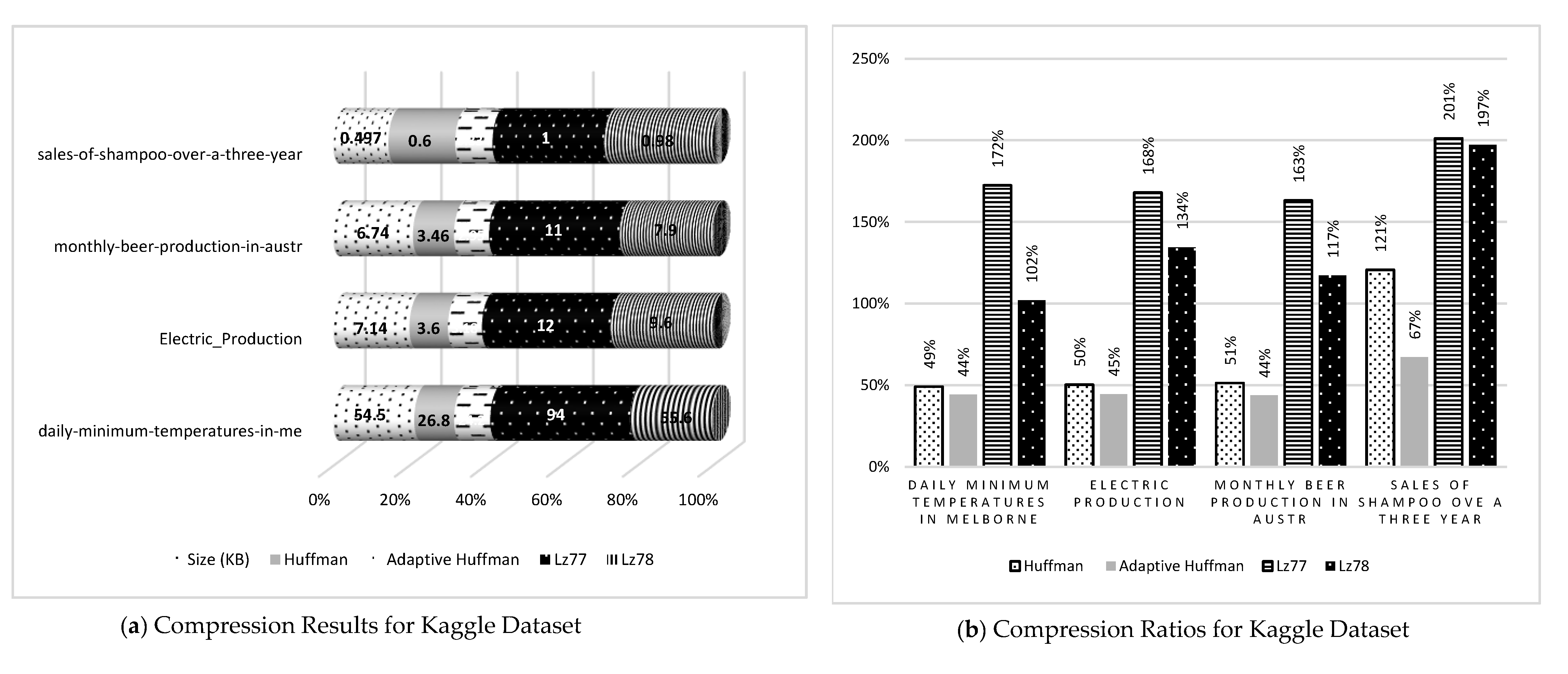
| Kaggle | 1 | Daily-minimum-temperatures-in-me | 54.500 | 26.800 | 49 | 24.200 | 44 | 94.000 | 172 | 55.600 | 102 |
| Kaggle | 1 | Electric_Production | 7.1400 | 3.600 | 50 | 3.180 | 45 | 12.000 | 168 | 9.600 | 134 |
| UCI | 1 | Monthly sunspots | 43.900 | 21.700 | 49 | 19.700 | 45 | 73.000 | 166 | 42.950 | 98 |
| UCI | 1 | Ozone level Detection 8 Hours | 799.000 | 346.000 | 43 | 346.000 | 43 | 1336.000 | 167 | 783.820 | 98 |
| UCI | 1 | Occupancy dataset | 196.000 | 95.500 | 49 | 95.200 | 49 | 331.000 | 169 | 191.623 | 98 |
| UCI | 1 | Ionosphere data | 74.600 | 33.800 | 45 | 33.700 | 45 | 125.000 | 168 | 89.480 | 120 |
| AMPDS | 1 | Climate hourly weather | 1413.120 | 697.000 | 49 | 680.000 | 48 | 2372.000 | 168 | 1004.170 | 71 |
| AMPDS | 1 | Climate historical normals | 2.580 | 1.940 | 75 | 1.610 | 62 | 4.000 | 155 | 4.200 | 163 |
| AMPDS | 1 | Electricity monthly | 0.735 | 0.781 | 106 | 0.489 | 67 | 1.000 | 136 | 1.550 | 211 |
| AMPDS | 1 | Natural gas monthly | 0.416 | 0.576 | 138 | 0.301 | 72 | 0.986 | 237 | 0.861 | 207 |
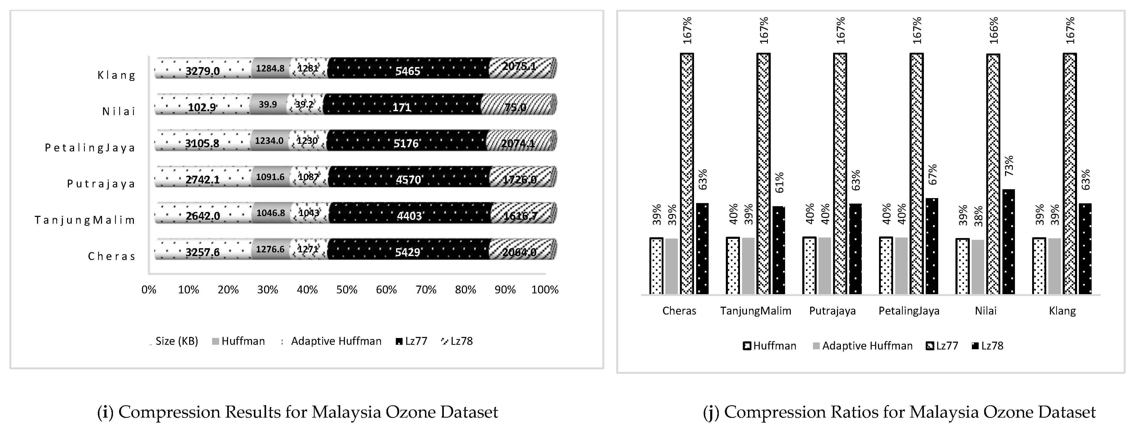
| Ozone | 1 | Cheras | 3257.585 | 1276.561 | 39 | 1271.000 | 39 | 5429.000 | 167 | 2063.960 | 63 |
| Ozone | 1 | TanjungMalim | 2641.970 | 1046.768 | 40 | 1043.000 | 39 | 4403.000 | 167 | 1616.730 | 61 |
| Ozone | 1 | Putrajaya | 2742.100 | 1091.609 | 40 | 1087.000 | 40 | 4570.000 | 167 | 1726.020 | 63 |
| Ozone | 1 | PetalingJaya | 3105.790 | 1234.014 | 40 | 1230.000 | 40 | 5176.000 | 167 | 2074.050 | 67 |
| Ozone | 1 | Nilai | 102.932 | 39.881 | 39 | 39.200 | 38 | 171.000 | 166 | 75.000 | 73 |
| Ozone | 1 | Klang | 3279.01 | 1284.780 | 39 | 1281.000 | 39 | 5465.000 | 167 | 2075.070 | 63 |
| Kaggle | 2 | Monthly beer production in Australia | 6.740 | 3.460 | 51 | 2.950 | 44 | 11.000 | 163 | 7.900 | 117 |
| Kaggle | 2 | Sales of shampoo over a three year period | 0.497 | 0.600 | 121 | 0.334 | 67 | 1.000 | 201 | 0.980 | 197 |
| UCI | 2 | Daily total female births | 6.070 | 2.990 | 49 | 2.590 | 43 | 10.000 | 165 | 5.500 | 91 |
| AMPDS | 2 | Electricity billing | 1.740 | 1.270 | 73 | 0.965 | 55 | 3.000 | 172 | 3.250 | 187 |
| AMPDS | 2 | Water billing | 0.180 | 0.344 | 191 | 0.135 | 75 | 0.474 | 263 | 0.421 | 234 |
| Corpus | 3 | bib | 108.653 | 71.700 | 66 | 71.200 | 66 | 193.000 | 178 | 144.443 | 133 |
| Corpus | 3 | book1 | 750.753 | 428.000 | 57 | 428.000 | 57 | 291.000 | 39 | 242.690 | 32 |
| Corpus | 3 | book2 | 596.539 | 360.000 | 60 | 359.000 | 60 | 1023.000 | 171 | 752.284 | 126 |
| Corpus | 3 | news | 368.271 | 241.000 | 65 | 240.000 | 65 | 635.000 | 172 | 523.000 | 142 |
| Corpus | 3 | paper1 | 51.915 | 33.200 | 64 | 32.700 | 63 | 90.000 | 173 | 78.540 | 151 |
| Corpus | 3 | paper2 | 80.272 | 47.200 | 59 | 46.600 | 58 | 138.000 | 172 | 114.830 | 143 |
| Corpus | 3 | progc | 38.683 | 26.000 | 67 | 25.400 | 66 | 69.000 | 178 | 59.540 | 154 |
| Corpus | 3 | progl | 69.967 | 42.600 | 61 | 42.100 | 60 | 121.000 | 173 | 89.410 | 128 |
| Corpus | 3 | progp | 48.222 | 30.200 | 63 | 29.600 | 61 | 85.000 | 176 | 61.680 | 128 |
| Corpus | 3 | trans | 91.499 | 64.400 | 70 | 62.100 | 68 | 156.000 | 170 | 120.394 | 132 |
Publisher’s Note: MDPI stays neutral with regard to jurisdictional claims in published maps and institutional affiliations. |
© 2021 by the authors. Licensee MDPI, Basel, Switzerland. This article is an open access article distributed under the terms and conditions of the Creative Commons Attribution (CC BY) license (https://creativecommons.org/licenses/by/4.0/).
Share and Cite
Nasif, A.; Othman, Z.A.; Sani, N.S. The Deep Learning Solutions on Lossless Compression Methods for Alleviating Data Load on IoT Nodes in Smart Cities. Sensors 2021, 21, 4223. https://doi.org/10.3390/s21124223
Nasif A, Othman ZA, Sani NS. The Deep Learning Solutions on Lossless Compression Methods for Alleviating Data Load on IoT Nodes in Smart Cities. Sensors. 2021; 21(12):4223. https://doi.org/10.3390/s21124223
Chicago/Turabian StyleNasif, Ammar, Zulaiha Ali Othman, and Nor Samsiah Sani. 2021. "The Deep Learning Solutions on Lossless Compression Methods for Alleviating Data Load on IoT Nodes in Smart Cities" Sensors 21, no. 12: 4223. https://doi.org/10.3390/s21124223
APA StyleNasif, A., Othman, Z. A., & Sani, N. S. (2021). The Deep Learning Solutions on Lossless Compression Methods for Alleviating Data Load on IoT Nodes in Smart Cities. Sensors, 21(12), 4223. https://doi.org/10.3390/s21124223