Abstract
Vehicle parameters are essential for dynamic analysis and control systems. One problem of the current estimation algorithm for vehicles’ parameters is that: real-time estimation methods only identify parts of vehicle parameters, whereas other parameters such as suspension damping coefficients and suspension and tire stiffnesses are assumed to be known in advance by means of an inertial parameter measurement device (IPMD). In this study, a fusion algorithm is proposed for identifying comprehensive vehicle parameters without the help of an IPMD, and vehicle parameters are divided into time-independent parameters (TIPs) and time-dependent parameters (TDPs) based on whether they change over time. TIPs are identified by a hybrid-mass state-variable (HMSV). A dual unscented Kalman filter (DUKF) is applied to update both TDPs and online states. The experiment is conducted on a real two-axle vehicle and the test data are used to estimate both TIPs and TDPs to validate the accuracy of the proposed algorithm. Numerical simulations are performed to further investigate the algorithm’s performance in terms of sprung mass variation, model error because of linearization and various road conditions. The results from both the experiment and simulation show that the proposed algorithm can estimate TIPs as well as update TDPs and online states with high accuracy and quick convergence, and no requirement of road information.
1. Introduction
Parameters are very important for dynamic analysis and control systems [1], as the accuracy of parameters directly determines the precision of the analysis results [2,3] and the performance of control systems [4,5]. Parameters can be divided into time-independent parameters (TIPs) and time-dependent parameters (TDPs) based on whether they change over time. TIPs are fixed values specified by a vehicle manufacturer, including inertial parameters of empty vehicles, suspension damping coefficients and suspension and tire stiffnesses. By contrast, TDPs can vary during a trip, including real-time sprung mass, center of gravity (CG) and moment of inertia (MI).
An inertial parameter measurement device (IPMD) is a highly specialized test device for the measurement of vehicle TIPs, and thus is expensive [6]. Generally, TIPs can be supplied by the vehicle manufacturer. But for a situation where TIPs are not supplied, an estimation method of TIPs without limitation of the IPMD would be practical and easy to use. Zheng et al. [7] suggest an estimation process of parameters based on the free-decay responses of the vehicle; the test can be performed on anywhere existing a short stage. If the modal parameters are obtained, then the gross mass, suspension damping coefficients and suspension and tire stiffnesses can be determined by a fitting process. The modal parameter identification methods can be divided into frequency-domain methods and time-domain methods. As the modal frequencies of the vehicle body are typically in 1–3 Hz, which is a small range, frequency domain methods are limited, whereas time domain methods are more appropriate to identify the modal parameters [8].
Relatively, TDPs’ estimation is more challenging as an online process is necessary. For example, although the mass and CG can be calculated using a static weighing scale, the online information of the vehicle mass is hard to know due to pick-ups or drop-offs during a trip and dynamic behaviors in motion. Rozyn and Zhang [9] suggested an updated TDP method with the sprung mass response by extracting equivalent free-decay responses, which essentially is still based on the identification of modal parameters. The limitation of this method is that extraction of free-decay responses will affect real-time performance.
Real-time estimation methods for some of the vehicle parameters have been suggested by numerous studies. Recursive least square (RLS) is a popular one for vehicle mass, which utilizes maximum likelihood theory [10,11,12,13]. A Kalman filter (KF) is also commonly used [14,15,16,17,18] as a special case of the recursive Bayesian estimation algorithm with assumptions of linear state-space representation and Gaussian probability distribution. However, both RLS and the KF are limited for linear systems, and hence, KF variants, such as extended KF [19,20,21,22,23] or unscented KF [24,25,26], are more suitable for nonlinear estimation. The extended KF usually provides “first-order” approximations to the optimal terms. While “second-order” versions of the extended KF exist, their increased implementation and computational complexity tend to prohibit their use. The unscented transform (UT) is a method for calculating the statistics of a random variable that undergoes a nonlinear transformation. In addition, a two-layer algorithm is also suggested: one layer is for vehicle parameters, while the other one is for states [24,27]. Therefore, a dual unscented KF method would be very useful to deal with both parameters and states for nonlinear systems.
The vehicle parameter estimation methodologies can also be classified based on the vehicle models used: longitudinal, yaw, roll and bounce. The most prevalent methods in preview studies are based on the longitudinal one [10,11,12,13,28], which appears simple though is practically limited by access to input forces, such as changing vehicle gravity, aerodynamic drag and road friction. In addition, only vehicle mass but neither CG nor MI can be estimated by the longitudinal model method. The yaw and roll models are also popular [19,24,29,30] but their accuracy is significantly dependent on the accuracy of the tire model, which is highly variable according to tire brand, wear and inflation pressures. Theoretically, both the vehicle parameters and suspension states can be accurately estimated through a vertical model [9], but few studies for vehicle parameter estimation are found using this kind of model. Boada et al. [29] estimated mass through a vertical model, but they ignored the variation of CG and MI when load mass changed. Zhou et al. [30] suggested a very interesting mass estimation method based on vertical suspension deflection recognition with cameras, but nevertheless averaged a 42.5% relative error, likely caused by non-contact measurement.
Taking into consideration all the previous ideas, the primary objective of this study is to propose a comprehensive algorithm estimating TIPs as well as updating TDPs and online states with high accuracy and quick convergence. The contributions that clearly distinguish our endeavor from the aforementioned literature are that vehicle parameters are properly divided into TIPs and TDPs according to the requirement for updates, and consequently, different methods are formulated. TIPs can be determined offline based on the identification of modal parameters, while TDPs can be estimated online based on a real-time dual unscented Kalman filter (DUKF).
The outline of the paper is as follows. Section 2 formulates the vehicle model in vertical, pitch and roll dynamics. Section 3 describes the hybrid-mass state-variable (HMSV) method for TIPs’ estimation based on the identification of modal parameters. The structure of the DUKF for the online identification of TDPs and states is presented in Section 4. In Section 5, the proposed algorithm is verified by experimental data. Both a simulation and parameter study are shown in Section 6 to prove the algorithm’s performance in terms of sprung mass variation, model error because of linearization, and various road conditions. Our conclusion is summarized in Section 7.
2. Vehicle Model in Vertical and Pitch Dynamics
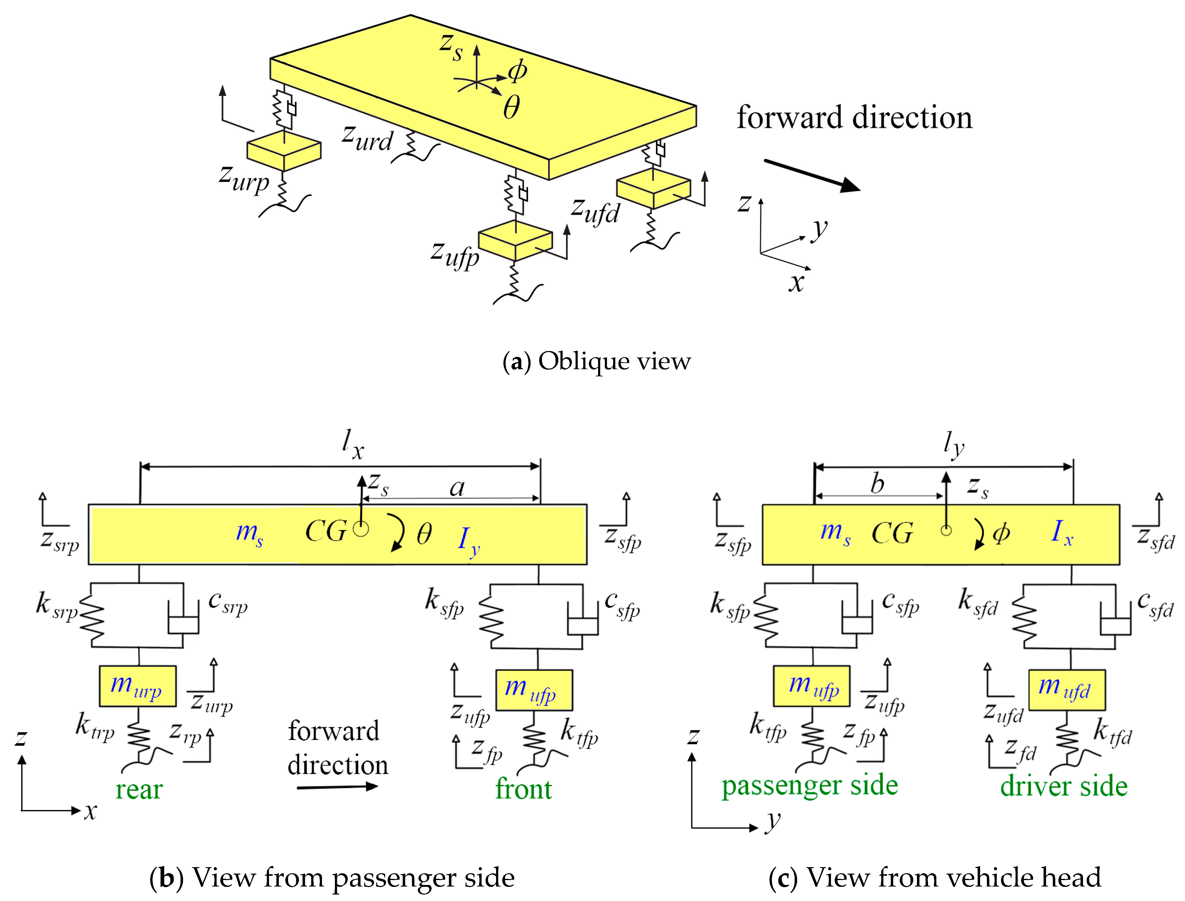
A full vehicle model comprising two axles is illustrated in Figure 1. The model consists of seven DOF (degrees of freedom), corresponding to the vertical motion of sprung mass , pitch motion of sprung mass , roll motion of sprung mass and vertical motions of four unsprung masses: , , and . The subscript stands for sprung mass, while is for unsprung mass, is for front axle, is for real axle, is for driver side and is for passenger side. () stands for the road profile input of each wheel. A detailed description of the vehicle parameters is given in Table A1 and Table A2 in Appendix A.

Figure 1.
Multi-body dynamics model of full vehicle.
The seven DOF vehicle model can be described by the following dynamic equation
where , and are acceleration, velocity and displacement vectors, respectively; , and are mass, damping and stiffness matrices, respectively; and vectors and stand for the external excitation and suspension nonlinear parts of the vehicle system, respectively. These matrices and vectors are given by:
where the superscript “T” denotes the transposition of a vector or matrix, “diag” stands for diagonal matrix and the matrices , , and are expressed as follows, respectively
3. HMSV for Time-Independent Parameters
In this section, the time-independent parameters (TIPs), listed in Table A1 in Appendix A, are determined by the hybrid-mass state-variable (HMSV) method.
3.1. State-Variable Method
The basic concept of HMSV is identifying parameters through modal parameters, and thus the state-variable (SV) method is embedded to determine the modal parameters, firstly.
Introducing state vector , Equation (1) can be converted to the state-space form:
where is the road input, is the suspension nonlinear force, and matrices and are
During the free decay response, the road input is . In addition, the vehicle suspension usually expresses a strong linear character around the working point, while the nonlinear part generally can be ignored in the vehicle models [31], therefore, assuming . Consequently, the state-space equation can be described in the discrete time domain:
where
is the sampling interval. A finite difference equation is constructed with the transition matrix as:
where represents the measure error matrix, and the state matrices and are defined as
N is the column number of . Based on the least squares method, the transition matrix can be determined by
Solving the eigenvalue problem of the transition matrix gives the eigenvalues and eigenvectors . Based on Equation (17), and the eigenvalues and eigenvectors of matrix can be calculated as
The matrix can be calculated by
where and are, respectively, the conjugate matrices of and :
3.2. Determining Parameters with HMSV Method
The state matrix of the original vehicle system can be solved by Equation (24) but it is still not possible to determinate the mass matrix , the damping coefficient matrix or the stiffness matrix of the vehicle by directly solving Equation (12) alone, as the number of equations is fewer than the number of unknowns. Therefore, a hybrid-mass state-variable (HMSV) method is suggested by putting additional mass into the original vehicle system [7], forming a new mass matrix . Then, the new state matrix can be represented as
Both in Equation (12) and in Equation (27) can be determined by the SV method. Set the submatrices and of and , respectively, are
Combining Equation (28) and Equation (29), there is
As the additional mass and position can be measured, is easily calculated. Therefore, the mass matrix can be derived by Equation (30). Substituting into Equation (12), the damping coefficient matrix and the stiffness matrix of the vehicle can be determined. Subsequently, all fixed parameters of Table A1 in Appendix A can be obtained, including the inertial parameters of the empty vehicle, suspension damping coefficients, suspension stiffnesses and tire stiffnesses.
4. DUKF for Time-Dependent Parameters and States
In this section, the estimation process for TDPs and states using a DUKF method are formulated in detail. For a changing loading condition, all TDPs—, , , , and (listed in Table A2 in Appendix A)—are time-dependent and need to be estimated in real-time. Among them, , and are firstly estimated by the DUKF method, and then online MIs and can be calculated by the relationship between these vehicle inertial parameters, so as to be less complex than all TDPs estimated together.
4.1. Relationship between Time-Dependent Parameters
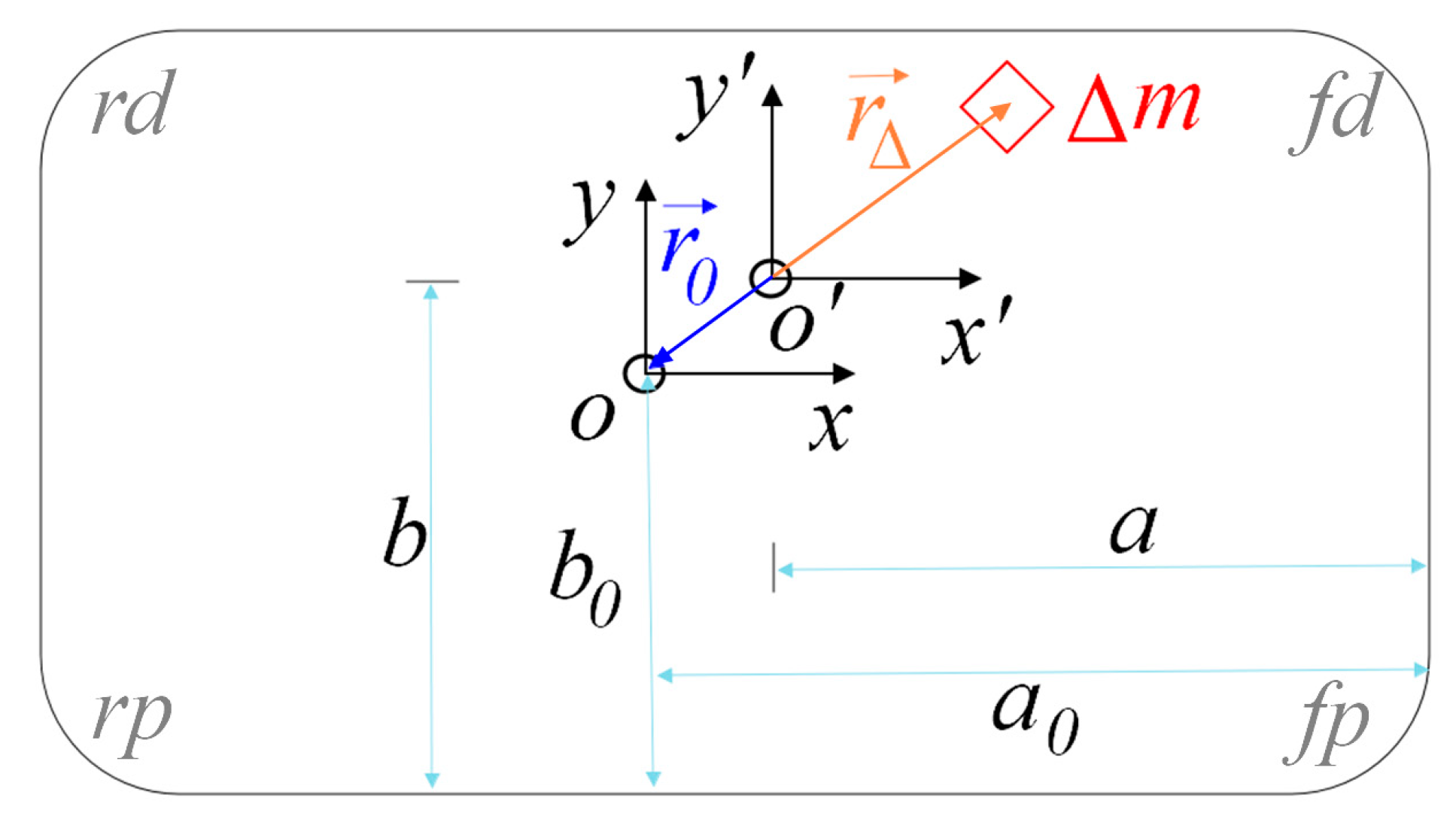
The additional mass is assumed as a rigid body, and it results in a new total sprung mass , as well as the new MIs ( and ) and the new CG displacements ( and ). The coordinate frame is at the original CG of the empty vehicle’s sprung mass, while the coordinate frame is at the new CG, as illustrated in Figure 2.

Figure 2.
Relationship between vehicle inertial parameters.
As shown in Figure 2, in the coordinate frame, , and are vectors from to o and added mass, respectively. As is the new mass center combining and , there will be , and thus , where and are unit vectors in the - and - directions, respectively. The added mass position can be expressed as
Using the parallel-axis theorem, the new MIs can be calculated as
Substituting Equation (31) and into Equation (32), the new MIs can be expressed by estimated , a and b as
4.2. Structure of Dual Unscented Kalman Filter
The structure of the DUKF is detailed herein based on the system model formulated in Section 2 and the SIPs determined in Section 3. Whilst a dual Kalman filter and dual extended Kalman filter were proposed by Wan and Nelson [32,33], they were applied to estimate vehicle states and part of the parameters by [19,24,29,34]. The DUKF in this paper uses the unscented KF (UKF) to ensure accuracy for both the linear and nonlinear systems. The DUKF is formed by two filters: the states UKF and the SIPs UKF.
The system equation for the states UKF is:
and the system equation for TDPs UKF is:
and are the process noise vector of states and TDPs, assumed to be zero mean Gaussian white noise with covariance and , respectively. , and is set to a large enough value, which is equal to 1000 in the later experiment and simulation; , where is about 1% of the corresponding initial value of TDPs [29]. The state vector for the states UKF is set as:
and () stand for the dynamic deflections of suspensions and tires, respectively. The sprung vertical displacement () at the top of each suspension can be expressed as:
In this way, the road profile inputs () are implicitly expressed as states in (), which can be estimated rather than required as an input for DUKF. Moreover, after a simplification by the relationship between the TDPs, the parameter vector for TDPs UKF is set as:
is the observation noise vector, assumed to be zero mean Gaussian white noise with covariance . There are , and , , () [34]. The output vector is set as:
where
UT is a method for calculating the statistics of a random variable that undergoes a nonlinear transformation, which is detailed in Appendix B. The DUKF consists of the prediction parts and the update parts, and the formulas of the DUKF for such a nonlinear system are stated in Appendix C step-by-step.
5. Framework of Proposed Algorithm and Experimental Verification
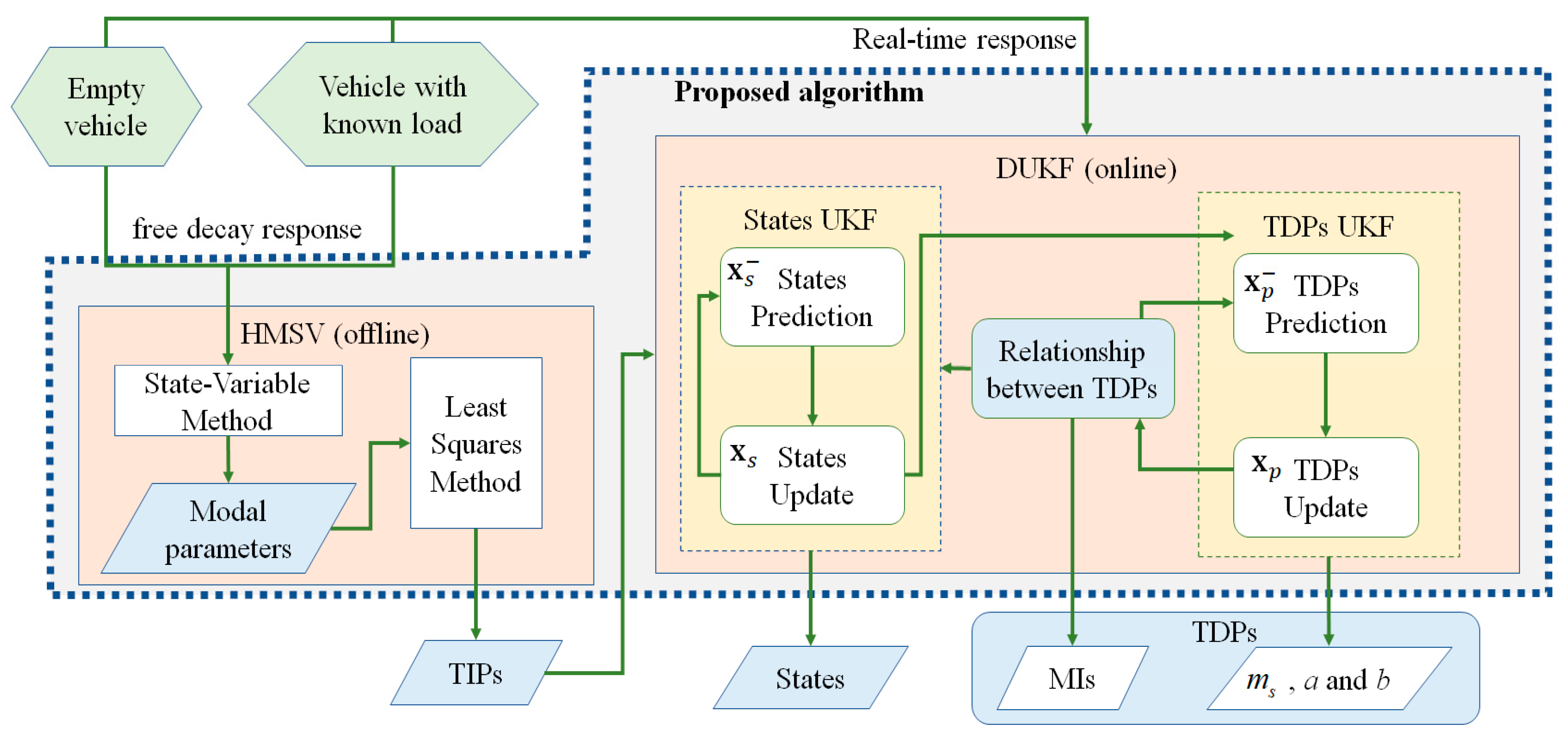
A comprehensive algorithm is proposed to estimate TIPs as well as update TDPs and online states. A flowchart of the proposed algorithm is shown in Figure 3. TIPs are estimated by HMSV based on the free decay response of an empty vehicle and a vehicle with a known load. Substituting the estimated TIPs into the DUKF, both the TDPs and states can be derived online according to the real-time dynamic response of vehicle in practical driving. An experiment is conducted to estimate both TIPs and TDPs and the test data are used to validate the accuracy of the proposed algorithm.
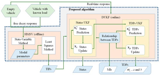
Figure 3.
Flowchart of proposed algorithm.
A stage-drop experiment by a real vehicle was performed, and the proposed algorithm, illustrated in Figure 3, was applied to estimate the vehicle parameters. Considering the dropping in the test as a kind of driving condition, the real-time response can be used to identify TDPs for vehicles with or without loads. The additional mass could be easily measured and was used to verify the accuracy of the proposed algorithm.
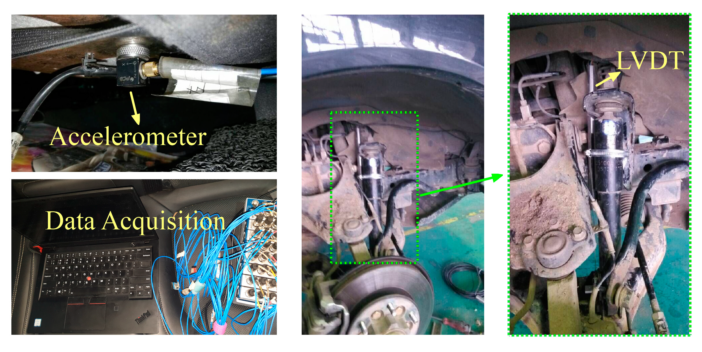
An experiment was performed on a two-axle vehicle equipped with a National Instruments Data Acquisition, enabling the synchronization and the evaluation of the logged data. There are four accelerometers and four linear variable differential transformer (LVDT) sensors used to provide data in the tests. The accelerometers are PCB PIEZOTRONICS’s 356A17 model, providing accurate measurements of three-axis accelerations with a resolution of 0.1 mg. In this work, only the vertical acceleration is taken into consideration. Four accelerometers are mounted on the chassis near four springs. Four LVDT sensors are mounted at each suspension to collect the dynamic deflections. The resolution of LVDT is about 0.1 um. One each of the mounted accelerometers and LVDTs are shown in Figure 4.

Figure 4.
Tested vehicle and equipment.
The free-decay tests are dividing into two groups, with or without loading. Each group of tests includes a bounce test, pitch test and roll test of the vehicle. In the bounce test, four wheels of the vehicle are dropped simultaneously off stages with the same height. In the pitch test, the front or rear wheels are dropped off stages to carry out the pitch mode. Similarly, in the roll test, the left or right wheels are dropped off stages to carry out the roll mode.
The wheel distance and axle distance are measured directly and the CG of the empty vehicle can be determined by static compression measurement as:
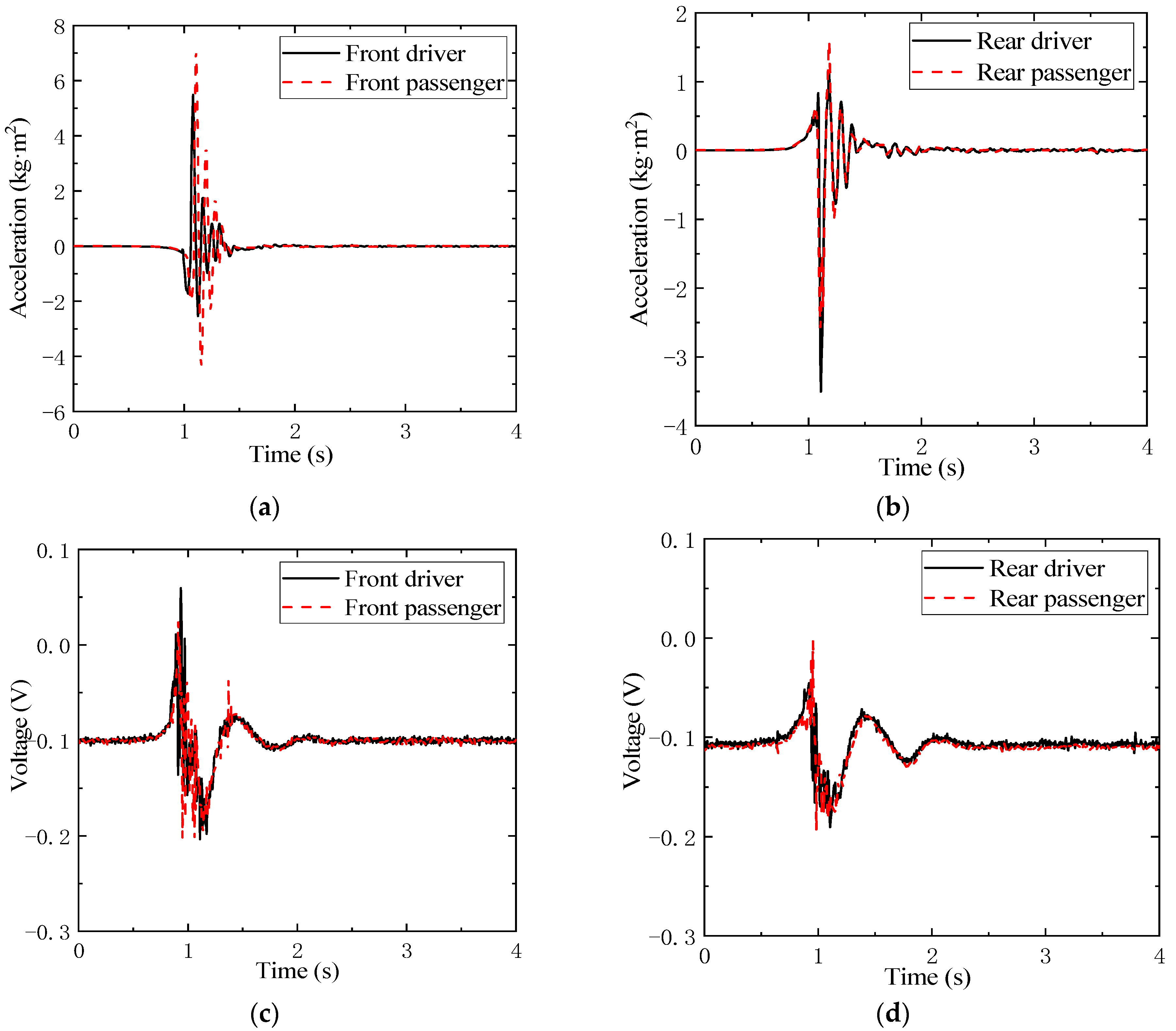
These determinable distances are listed in Table 1. Furthermore, the read data of accelerometers and LVDTs in a bounce test for an empty vehicle are illustrated in the Figure 5. It can be seen from Figure 5a,b that the acceleration values at the same axle are similar, while for a different axle they are diverse, which indicates similar stiffness and damping for suspensions at the same axle, but different suspension parameters for the front and rear axles. The data collected by LVDT are voltages, which can be transferred to compressions of each suspension.

Table 1.
Determinable distances and CG of empty vehicle.
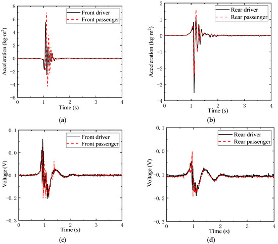
Figure 5.
Measured data of accelerometer (a,b) and LVDT (c,d) in bounce test for empty vehicle.
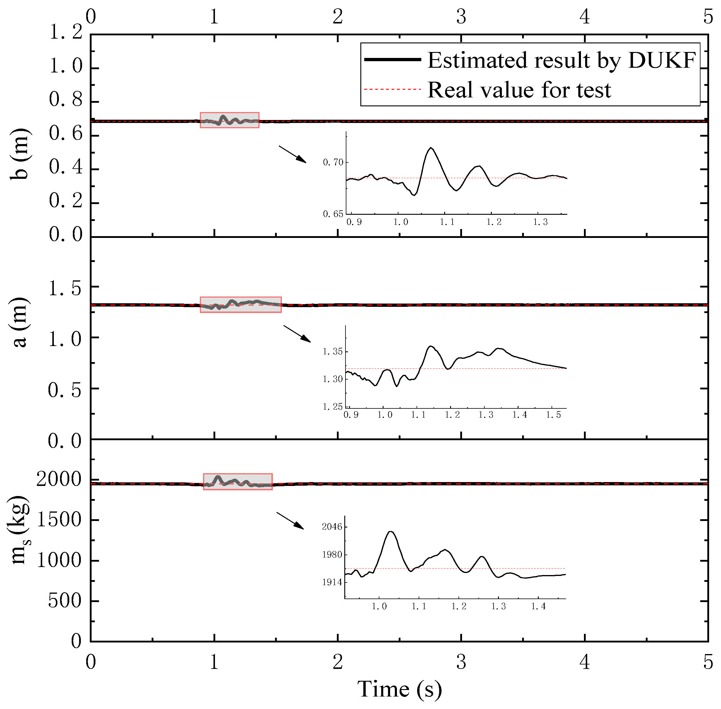
Based on above test data, TIPs can be estimated by the HMSV part, as are listed in Table 2. With these estimated TIPs, TDPs can be further estimated by the DUKF part. The estimated , and of the loading case are illustrated in Figure 6. The vehicle is in a steady state before 0.9 s and after 2 s, when a quite accurate mass and GC are obtained. It is worth noting that the dynamic deflections are nearly zero under a steady state, and Equation (40) gives the relationship between measured compressions and TDPs (mass and GC). In this way, TDPs can be estimated mainly according to the measured compression. This may be the reason why estimated TDPs keep nearly constant values for the steady state, considering that the data shown in Figure 5 are also smooth for the steady state. It can be seen from Figure 6 that the estimated values in the steady state are about 1948 kg, 1.32 mm and 0.68 mm, respectively. Furthermore, the additional mass for the loading case is 390 kg, put at the CG of the empty vehicle. The CG of the loading case equals that of the empty case, and thus the values of , , and would equal to , , and , respectively. Putting the estimated , and into Equation (36), the estimated and can be determined as 600 kg·m2 and 2381 kg·m2, respectively. The estimated . All these indicate that the estimated parameters match the test results well. From 0.9 s to 1.5 s, the vehicle dropped and bounced, and at this time, both the accelerometer and LVDT data vibrated significantly, corresponding to Figure 5, which leads to a slight vibration of the estimated TDPs in Figure 6. The proposed algorithm can suppress the dynamic vibration of measured data because the state vector in Equation (36) includes the dynamic behavior of the vehicle. It can be seen from Figure 6 that the estimation errors for TDPs are small. A worse road condition may boost the estimation errors; the effect of road conditions on estimation accuracy will be further studied in the next section by a simulation. The states cannot be measured directly in the test; their estimation will be further verified with simulation results.

Table 2.
Estimation results of TIPs with experimental data.
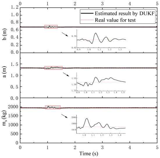
Figure 6.
Estimated TDPs by experimental data.
6. Performance Study of the Proposed Algorithm
In this section, further studies of the proposed algorithm are analyzed in terms of their ability to recognize the change of TDPs during a trip, the effect of nonlinear suspension properties and the performance on various road conditions, respectively. The simulations are implemented based on the vehicle model in Section 2. As TIPs will not change, these only need to be identified once and set as same for all cases. After each simulation, the estimation process is performed based on the set TIPs and the output vector in Equation (39). The accelerations and compressions of the output vector are calculated by adding Gaussian noise into the simulated sprung mass accelerations and suspension compressions, and the velocities of the output vector are obtained from the acceleration integral. TDPs and states change over time and are key to evaluate the algorithm’s performance.
6.1. Sprung Mass Variation
A simulation is performed for the shedding load at 4 s during the trip, with a driving speed 40 km/h on a rough road defined as road class B according to ISO 8608. Before shedding of the load happens, the load mass is 300 kg and corresponding , and . After shedding part of the load, the load mass is 150 kg and, correspondingly, , and .
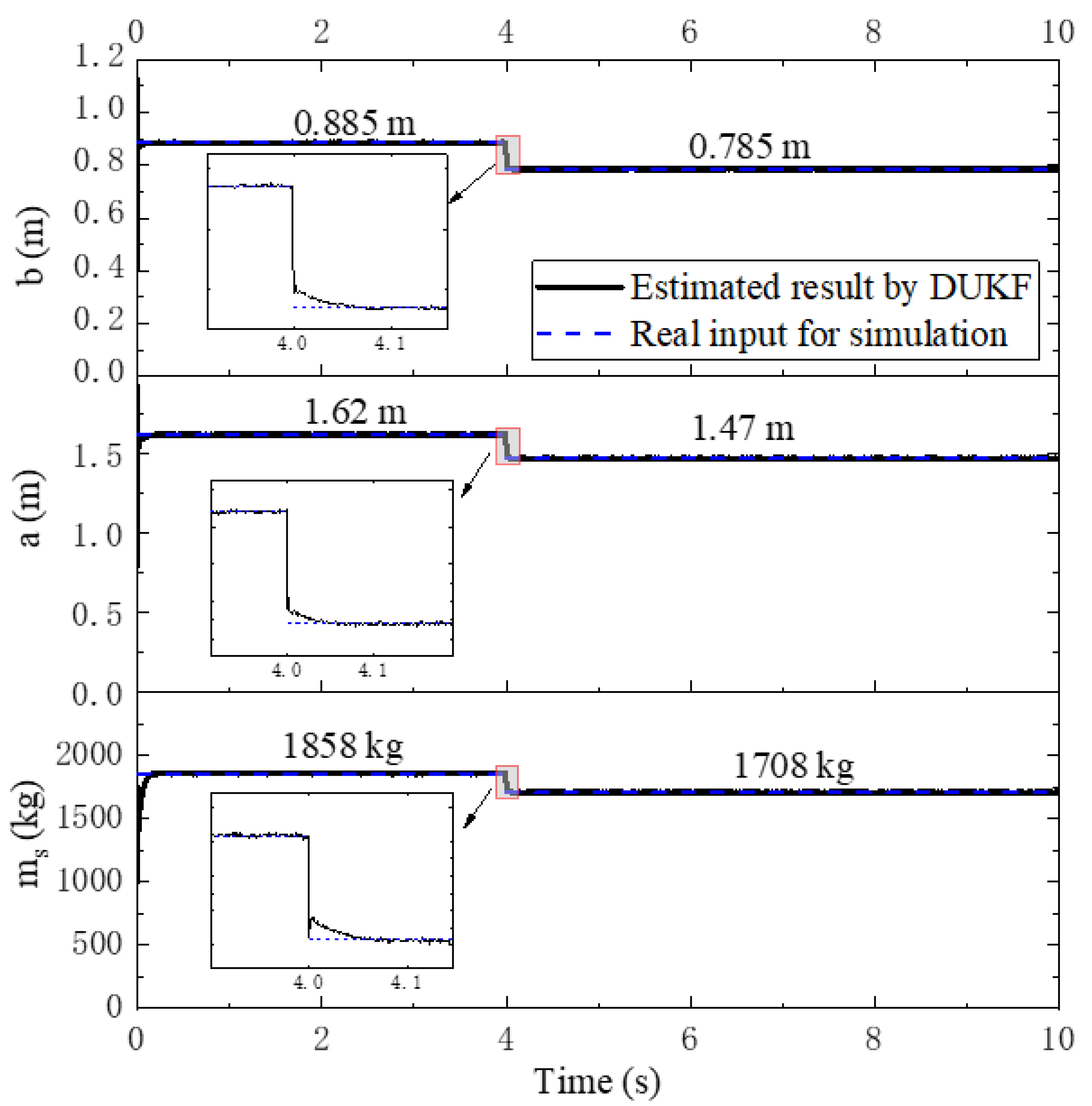
Comparisons of the , and values between the estimation and simulation are illustrated in Figure 7. Firstly, it can be seen that the estimated TDPs are nearly the same as the real input for the simulation if there is no change of loading, which means that the proposed algorithm is quite accurate for a class B road under 40 km/h. As the model used in the DUKF method accounts for the dynamic behavior of vehicle, the supposed algorithm can suppress the vibration. Secondly, at 4 s, shedding of the load happens and all TDPs change. It can be seen from Figure 7 that the proposed algorithm can detect the change of TDPs immediately, and approach the real input for simulation in about 0.05 s, which is quick enough for practical application.
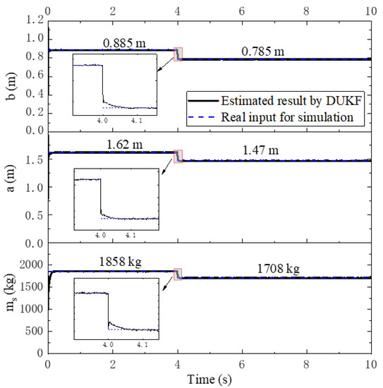
Figure 7.
TDPs for simulation and estimation in the shedding load scenario.
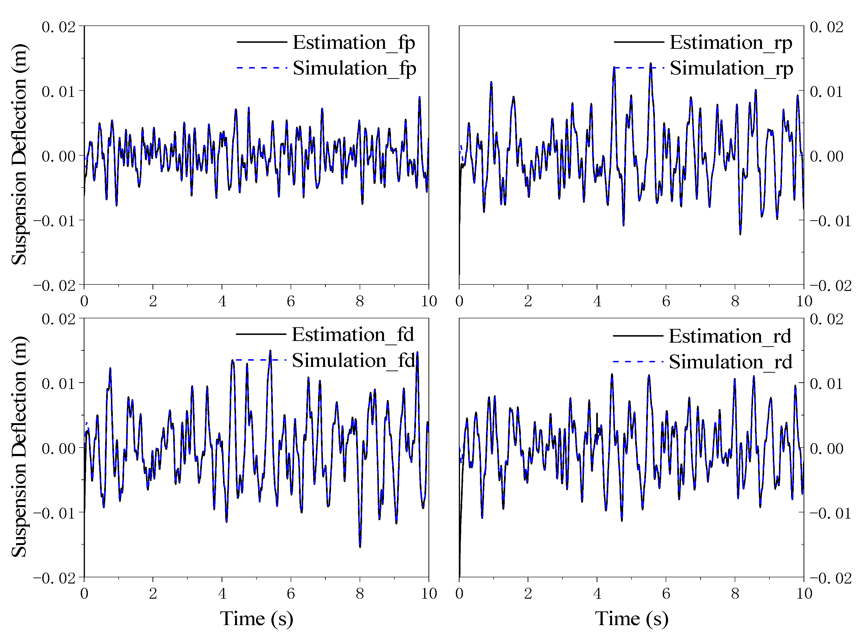
The dynamic deflections for the four suspensions can be estimated by DUKF, and their values in the mass change scenario are illustrated in Figure 8. It can be seen that the estimated values are nearly the same as the real inputs in the simulation, and even shedding a load at 4 s does not affect the estimated value by much. There is an approaching process happening near 0 s, which is because of the difference between the given initial values for DUKF and the real initial values in the simulation.
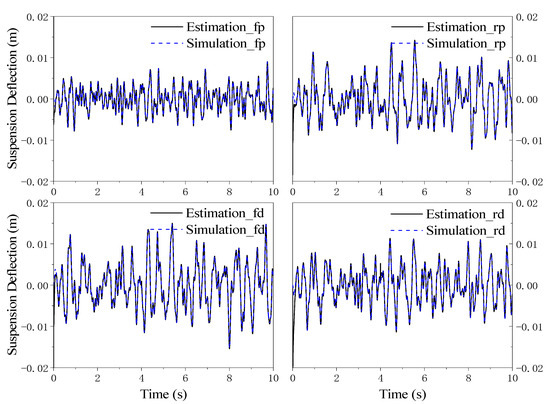
Figure 8.
Suspension deflection for simulation and estimation in the shedding load scenario.
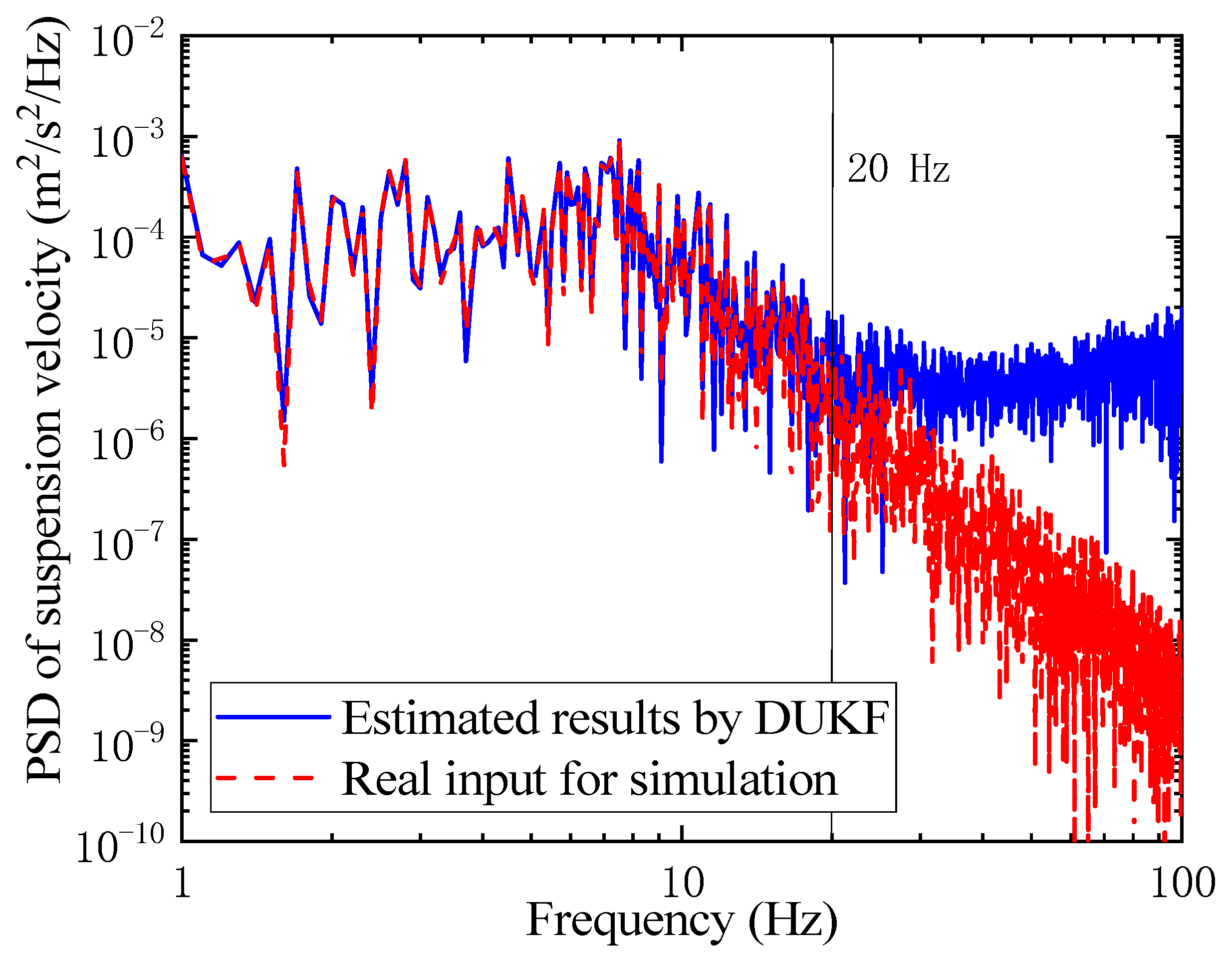
The suspension velocity can be estimated by the states UKF of the DUKF part in Figure 3. The power spectral density (PSD) values of the suspension velocity for the simulation and estimation are compared in Figure 9. It is clear that the estimated suspension velocity can approximate the real input for the simulation below 20 Hz, but in the higher frequency area, the estimated value is larger than the real input for the simulation.
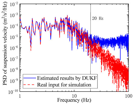
Figure 9.
PSD of suspension velocity for simulation and estimation.
Tire deflection can also be estimated by the DUKF part without road information. The PSDs of tire deflection for the simulation and estimation are shown in Figure 10, and it can be seen that the estimated tire deflection can approximate the real input for the simulation between 3 Hz and 20 Hz. The region of greatest human sensitivity to vertical vibration lies between 4 and 8 Hz [35], while the natural frequency of wheel-hop is about 12 Hz [36], both of which are in the relatively accurate region in Figure 10. Hence, the proposed algorithm can determine accurate tire deflection information in these frequency regions of concern.
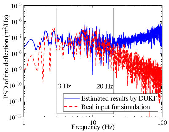
Figure 10.
PSD of tire deflection for simulation and estimation.
6.2. Effect of Vehicle Model Linearization
The vehicle model given in Section 2 has linear stiffness and damping, but in reality, they are usually nonlinear [37]. Therefore, it is necessary to study the effect of linearization on the estimation results. The nonlinear part of the suspension reaction forces can be expressed as [38]:
where is the nonlinear part of suspension stiffness and and are coefficients of suspension nonlinear damping.
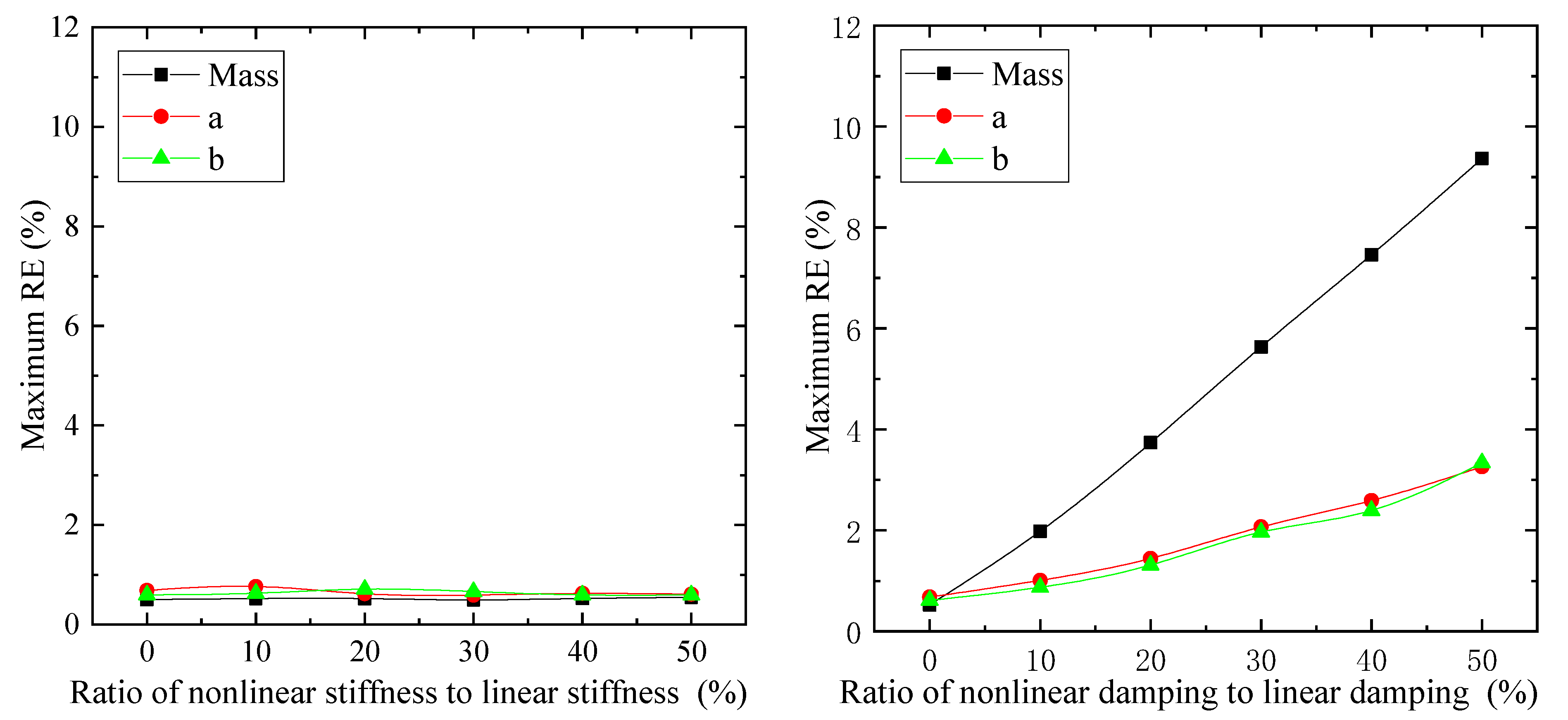
In the simulations, the nonlinear parts of the suspension—, and —are considered variables and the ratios of them to their corresponding linear parts are set from 0 percent to 50 percent, while for the estimation, only linear part values are taken into consideration. The relative error (RE) between the estimation and simulation values can be expressed as
The RE between the estimation and simulation represents the accuracy of the proposed estimation algorithm, and the maximum REs of the TDPs are illustrated in Figure 11. It can be seen that various ratios of nonlinear stiffness to linear stiffness lead to a similar maximum RE (below 1%), whereas larger nonlinear damping causes higher RE values for TDPs. This means that disregard for nonlinear damping rather than nonlinear stiffness in the estimation process would affect the accuracy of TDPs. The reason could be that suspension deflections can be determined directly by the measured compressions, but the suspension velocity cannot. Accordingly, the incorrect stiffness value can be partly improved by the accurate suspension deflections with the help of the DUKF, whereas both the suspension velocity and the damping values are not accurate, which would lead to a large error eventually.
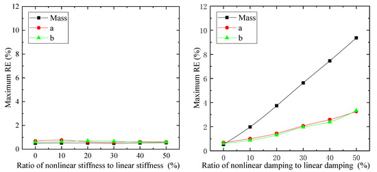
Figure 11.
Maximum RE of TDPs for various ratios of nonlinear part to linear part for suspension properties.
6.3. Performance under Various Road Conditions
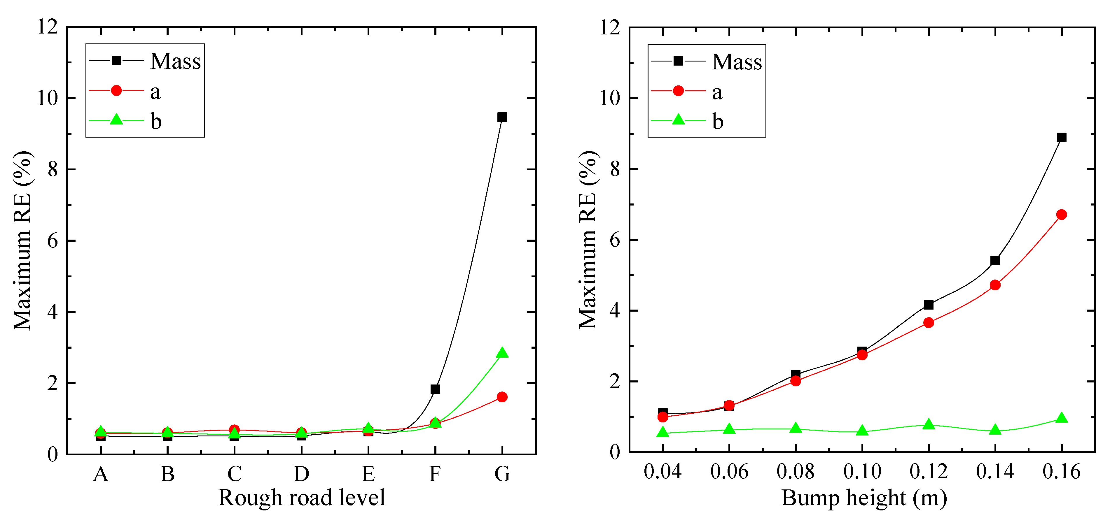
In order to study the performance of the proposed estimation method under various road conditions, the simulations are implemented on various road roughness levels (according to ISO 8608) and speed bump heights. After that, the estimation process is performed based on the simulated results. A driving speed of 40 km/h and sprung mass of 2000 kg are considered for all cases. The RE values are calculated based on the simulation and estimation results, and the maximum REs are illustrated in Figure 12. It can be seen that the proposed algorithm can maintain accurate estimation results with REs of below 5% until road roughness level F. Even though the maximum REs of reach about 10% for level G, in practice, it rarely happens that a vehicle is driving on level G under 40 km/h [39]. For the speed bump cases, the maximum REs of and increase with speed bump height. A commonly used height for speed bump is 0.07 m, on which the RE is below 2%. does not change much; this is because vehicle is driven with two coaxial wheels travelling across the speed bump together. In total, the proposed algorithm can estimate TDPs with REs of below 2% for road roughness level F and speed bump height 0.07 m, under 40 km/h.
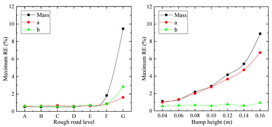
Figure 12.
Maximum RE of TDPs for various ratios of nonlinear part to linear part for suspension properties.
6.4. Feasibility of the Algorithm for Updating TDPs
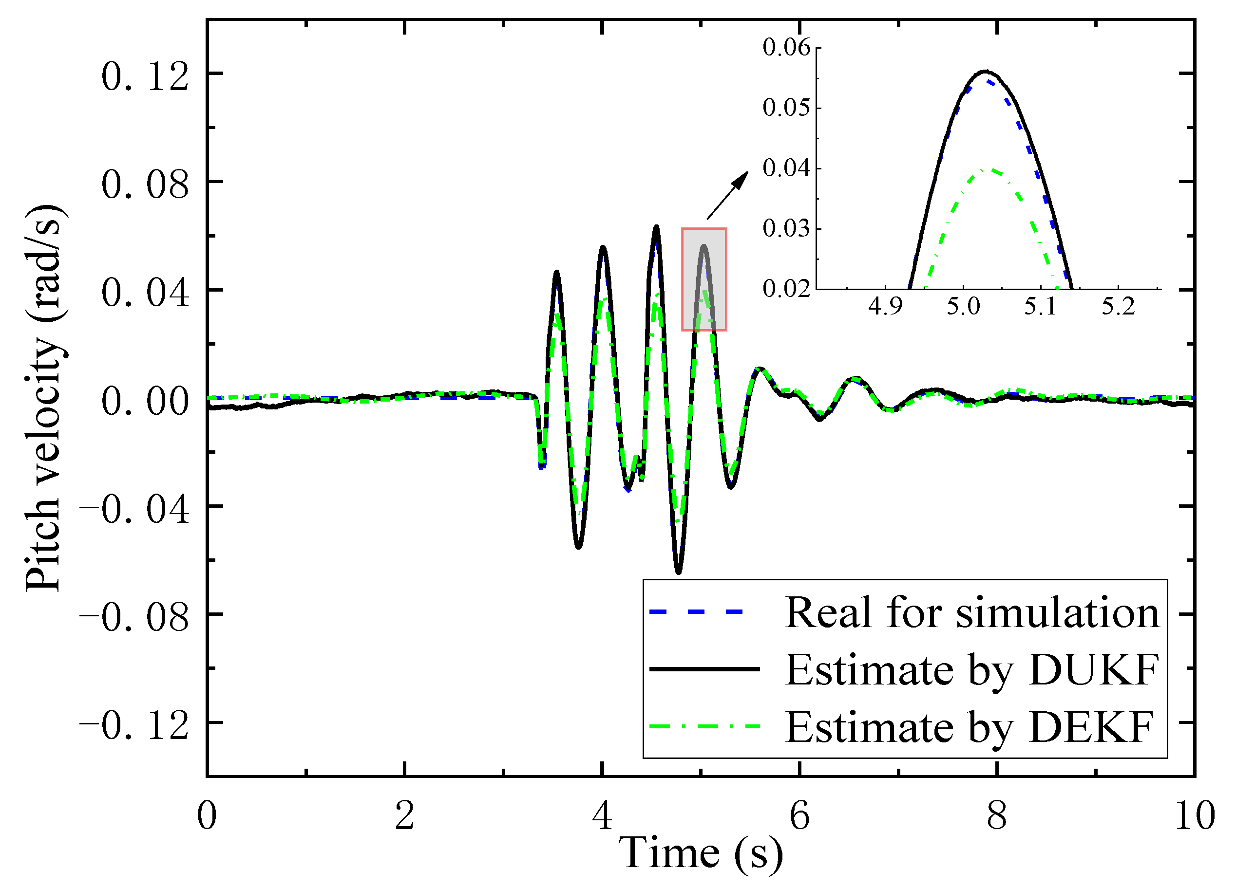
The feasibility of the proposed algorithm from the implementation and computational point in practice is a very important question, and it is necessary to be studied. Therefore, we have illustrated a pitch velocity with real data in a simulation and estimated the results using the DUKF in Figure 13, where the results using the dual extended KF (DEKF) are compared to them. A detailed estimating process of the DEKF can be found in [40]. The simulation is conducted on a bumpy road (0.4 m height and 0.35 m width) under 10 km/h with a ratio of nonlinear stiffness force of 50% to the linear part. It can be seen from Figure 13 that the estimation errors by the DUKF are much smaller than that by the DEKF during the estimation process. The phenomenon can be explained by the DEKF using the linearization of Jacobian matrices with high-order truncation error to approximate the non-linear estimation system. Similar results for the comparison of accuracy between the DUKF and DEKF can also be found in [40].
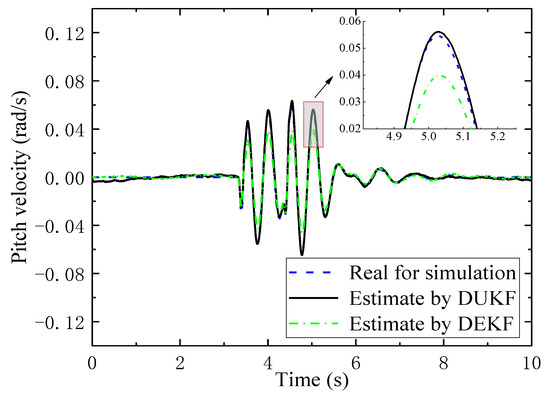
Figure 13.
Comparison of the DUKF and DEKF estimating results.
For the 10 s simulation, the estimation of the DUKF uses 10.083 s to finish the estimation. It means the DUKF has a high possibility of updating TDPs online in practice. However, for the same simulation, the DEKF costs 2499.167 s. The most time-consuming process is the derivation of Jacobian matrices (2490.985 s) as there are fifteen variants in our state vector (Equation (36)), three variants in our parameter vector (Equation (38)) and twelve variants in our output vector (Equation (39)).
7. Conclusions
Identification of vehicle parameters is essential for dynamic analysis and control systems. This study is aimed to propose a fusion algorithm for identifying comprehensive vehicle parameters without the help of an inertial parameter measurement device (IPMD). This paper divides the parameters of the vehicle into time-independent parameters (TIPs) and time-dependent parameters (TDPs) based on whether or not they change over time. The novelty of this paper is providing a comprehensive algorithm to estimate TIPs as well as update TDPs and online states for vehicle. TIPs were identified firstly by means of a hybrid-mass state-variable (HMSV) method. With the estimated values of TIPs, a dual unscented Kalman filter (DUKF), consisting of two parallel layers running simultaneously, was constructed to estimate both TDPs and online states. Experiments were conducted to estimate both TIPs and TDPs and so as to validate the accuracy of proposed algorithm. Numerical simulations were performed to further investigate the DUKF’s performance in terms of sprung mass variation, model error during linearizing and various road conditions. The results from both the experiment and the simulation showed that the proposed algorithm could estimate TIPs as well as update TDPs and online states with high accuracy and no requirement of the road information.
With the proposed method, vehicle parameters can be identified separately and accurately. TIPs can be identified offline and stored for further use, while only TDPs are updated online, which improves the efficiency of estimation. In addition, it worth noting that by including the relationship between dynamic states and compression, the accuracy of the proposed method is quite high except for under significant dynamics caused by very bad road conditions, such as Class G roads or high bumps. We are now interested in extending the method for other mechanical systems in the future.
Author Contributions
Conceptualization, Z.Z.; methodology, Z.Z.; validation, Z.Z.; formal analysis, Z.Z. and J.D.; investigation, J.D.; data curation, J.D. and H.Q.; writing—original draft preparation, Z.Z.; writing—review and editing, J.Z.; supervision, B.Z.; funding acquisition, J.Z. and B.Z. All authors have read and agreed to the published version of the manuscript.
Funding
This research was partly supported by the National Natural Science Foundation of China [grant numbers 51875181, 12002123], the Natural Science Foundation of Hunan Province [grant number 2020JJ5079] and the Open Fund of the State Key Laboratory of Advanced Design and Manufacturing for the Vehicle Body [grant number 32065011].
Conflicts of Interest
The authors declare no conflict of interest.
Nomenclature
| Notation | Description |
| Vertical Displacement | |
| Pitch Motion | |
| Roll Motion | |
| Acceleration Vector | |
| Velocity Vector | |
| Displacement Vector | |
| Mass Matrix | |
| Damping Matrix | |
| Stiffness Matrix | |
| Force Matrix | |
| State Vector | |
| Coefficient Matrix | |
| State Matrices | |
| Sampling Interval | |
| Measure Error Matrix | |
| Eigenvalue | |
| Eigenvector | |
| Subscript | |
| Sprung Mass | |
| Unsprung Mass | |
| Front Axle | |
| Real Axle | |
| Driver Side | |
| Passenger Side | |
| External Excitation | |
| Nonlinear Part | |
| New Mass | |
| Superscript | |
| Submatrices | |
| Conjugate Matrices |
Appendix A. Vehicle Parameters

Table A1.
Fixed parameters for vehicle.
Table A1.
Fixed parameters for vehicle.
| Parameter | Description | Unit |
|---|---|---|
| Empty sprung mass | kg | |
| Roll MI of empty sprung mass | ||
| Pitch MI of empty sprung mass | ||
| () | Unsprung mass | kg |
| () | Stiffness of suspension spring | N/m |
| () | Stiffness of tire | N/m |
| () | Damping of suspension | |
| Axle distance | m | |
| Wheel distance at same axle | m | |
| Distance from CG to front axle for empty vehicle | m | |
| Distance from CG to passenger side wheel line for empty vehicle | m |

Table A2.
Time-dependent parameters for vehicle.
Table A2.
Time-dependent parameters for vehicle.
| Parameter | Description | Unit |
|---|---|---|
| Total sprung mass | kg | |
| Additional sprung mass | kg | |
| Roll MI of real-time sprung mass | ||
| Pitch MI of real-time sprung mass | ||
| Distance from real-time CG to front axle | m | |
| Distance from real-time CG to passenger side wheel line | m |
Appendix B. Unscented Transform
The unscented transform (UT) is used to deal with the nonlinear part. Using state UT as an example, the 2N + 1 sigma points are chosen as:
N is the dimension of the state vector ; is a scaling parameter, user-defined [41]; the constant is usually set as , determining the spread of the sigma around the mean of these sigma points ; can make sure that the covariance matrix is definitely positive. The weights of the sigma points are calculated as:
considers the high-order moment of the prior distribution, and it is optimally set as 2 for Gaussian distribution.
Appendix C. Formulas of the DUKF
The DUKF consists of the prediction parts and the update parts, and the formulas of the DUKF for such a nonlinear system are stated here step-by-step:
Step 1. State prediction
Step 2. State measure update
Step 3. State update
Step 4. SIP prediction
Step 5. SIP measure update
Step 6. SIP update
where and are the dimensions of the state vector and parameter vector, respectively. are measurement data.
References
- Shokravi, H.; Shokravi, H.; Bakhary, N.; Heidarrezaei, M.; Rahimian Koloor, S.S.; Petrů, M. A review on vehicle classification and potential use of smart vehicle-assisted techniques. Sensors 2020, 20, 3274. [Google Scholar] [CrossRef]
- Zhang, Z.; Dhanasekar, M.; Ling, L.; Thambiratnam, D.P. Effectiveness of a raised road: Rail crossing for the safety of road vehicle occupants. Eng. Fail. Anal. 2019, 97, 258–273. [Google Scholar] [CrossRef]
- Hsu, L.-Y.; Chen, T.-L. Vehicle dynamic prediction systems with on-line identification of vehicle parameters and road conditions. Sensors 2012, 12, 15778–15800. [Google Scholar] [CrossRef]
- Zhu, Q.; Li, L.; Chen, C.-J.; Liu, C.-Z.; Hu, G.-D. A low-cost lateral active suspension system of the high-speed train for ride quality based on the resonant control method. IEEE Trans. Ind. Electron. 2017, 65, 4187–4196. [Google Scholar] [CrossRef]
- Gao, L.; Xiong, L.; Lin, X.; Xia, X.; Liu, W.; Lu, Y.; Yu, Z. Multi-sensor fusion road friction coefficient estimation during steering with lyapunov method. Sensors 2019, 19, 3816. [Google Scholar] [CrossRef]
- Zagorski, S.; Heydinger, G.; Coyle, J.; Jebode, M. Measured vehicle inertial parameters–NHTSA’s data through June 2020. SAE Technical Paper No. 2021-01-0970. 2021. Available online: https://saemobilus.sae.org/content/2021-01-0970/ (accessed on 12 June 2021).
- Zheng, M.; Zhang, B.; Zhang, J.; Zhang, N. Physical parameter identification method based on modal analysis for two-axis on-road vehicles: Theory and simulation. Chin. J. Mech. Eng. 2016, 29, 756–764. [Google Scholar] [CrossRef]
- Zheng, M.; Peng, P.; Zhang, B.; Zhang, N.; Wang, L.; Chen, Y. A new physical parameter identification method for two-axis on-road vehicles: Simulation and experiment. Shock. Vib. 2015, 2015, 1–9. [Google Scholar] [CrossRef]
- Rozyn, M.; Zhang, N. A method for estimation of vehicle inertial parameters. Veh. Syst. Dyn. 2010, 48, 547–565. [Google Scholar] [CrossRef]
- Bae, H.S.; Ryu, J.; Gerdes, J.C. Road grade and vehicle parameter estimation for longitudinal control using GPS. In Proceedings of the IEEE Conference on Intelligent Transportation Systems, Oakland, CA, USA, 25–29 August 2001; pp. 25–29. [Google Scholar]
- Vahidi, A.; Stefanopoulou, A.; Peng, H. Recursive least squares with forgetting for online estimation of vehicle mass and road grade: Theory and experiments. Veh. Syst. Dyn. 2005, 43, 31–55. [Google Scholar] [CrossRef]
- Lin, N.; Zong, C.; Shi, S. The method of mass estimation considering system error in vehicle longitudinal dynamics. Energies 2018, 12, 52. [Google Scholar] [CrossRef]
- Kidambi, N.; Pietron, G.M.; Boesch, M.; Fujii, Y.; Wang, K.-W. Accuracy and robustness of parallel vehicle mass and road grade estimation. SAE Int. J. Veh. Dyn. Stability, NVH 2017, 1, 317–325. [Google Scholar] [CrossRef]
- Zhang, J.; Ding, F.; Zhang, N.; Chen, S.; Zhang, B. A New SSUKF observer for sliding mode force tracking H∞ control of electrohydraulic active suspension. Asian J. Control. 2020, 22, 761–778. [Google Scholar] [CrossRef]
- Zhao, B.; Nagayama, T.; Xue, K. Road profile estimation, and its numerical and experimental validation, by smartphone measurement of the dynamic responses of an ordinary vehicle. J. Sound Vib. 2019, 457, 92–117. [Google Scholar] [CrossRef]
- Joa, E.; Yi, K.; Hyun, Y. Estimation of the tire slip angle under various road conditions without tire–road information for vehicle stability control. Control. Eng. Pr. 2019, 86, 129–143. [Google Scholar] [CrossRef]
- Reina, G.; Messina, A. Vehicle dynamics estimation via augmented Extended Kalman Filtering. Measurements 2019, 133, 383–395. [Google Scholar] [CrossRef]
- Salt Ducajú, J.M.; Salt Llobregat, J.J.; Cuenca, Á.; Tomizuka, M. Autonomous ground vehicle lane-keeping lpv model-based control: Dual-rate state estimation and comparison of different real-time control strategies. Sensors 2021, 21, 1531. [Google Scholar] [CrossRef]
- Wenzel, T.A.; Burnham, K.J.; Blundell, M.V.; Williams, R.A. Dual extended Kalman filter for vehicle state and parameter estimation. Veh. Syst. Dyn. 2006, 44, 153–171. [Google Scholar] [CrossRef]
- Huang, X.; Wang, J. Real-time estimation of center of gravity position for lightweight vehicles using combined AKF–EKF method. IEEE Trans. Veh. Technol. 2014, 63, 4221–4231. [Google Scholar] [CrossRef]
- Lin, C.; Gong, X.; Xiong, R.; Cheng, X. A novel H∞ and EKF joint estimation method for determining the center of gravity position of electric vehicles. Appl. Energy 2017, 194, 609–616. [Google Scholar] [CrossRef]
- Cai, L.; Wang, H.; Jia, T.; Peng, P.; Pi, D.; Wang, E. Two-layer structure algorithm for estimation of commercial vehicle mass. Proc. Inst. Mech. Eng. Part D J. Automob. Eng. 2019, 234, 378–389. [Google Scholar] [CrossRef]
- Sun, Y.; Li, L.; Yan, B.; Yang, C.; Tang, G. A hybrid algorithm combining EKF and RLS in synchronous estimation of road grade and vehicle׳ mass for a hybrid electric bus. Mech. Syst. Signal Process. 2016, 68–69, 416–430. [Google Scholar] [CrossRef]
- Hong, S.; Lee, C.; Borrelli, F.; Hedrick, J.K. A Novel approach for vehicle inertial parameter identification using a dual kalman filter. IEEE Trans. Intell. Transp. Syst. 2014, 16, 151–161. [Google Scholar] [CrossRef]
- Astroza, R.; Alessandri, A.; Conte, J.P. A dual adaptive filtering approach for nonlinear finite element model updating accounting for modeling uncertainty. Mech. Syst. Signal Process. 2019, 115, 782–800. [Google Scholar] [CrossRef]
- Wu, Q.; Jia, Q.; Shan, J.; Meng, X. Angular velocity estimation based on adaptive simplified spherical simplex unscented Kalman filter in GFSINS. Proc. Inst. Mech. Eng. Part G J. Aerosp. Eng. 2014, 228, 1375–1388. [Google Scholar] [CrossRef]
- Eftekhar Azam, S.; Chatzi, E.; Papadimitriou, C. A dual Kalman filter approach for state estimation via output-only acceleration measurements. Mech. Syst. Signal Process. 2015, 60–61, 866–886. [Google Scholar] [CrossRef]
- Li, B.; Zhang, J.; Du, H.; Li, W. Two-layer structure based adaptive estimation for vehicle mass and road slope under longitudinal motion. Measurement 2017, 95, 439–455. [Google Scholar] [CrossRef]
- Boada, B.L.; Boada, M.J.L.; Zhang, H. Sensor fusion based on a dual kalman filter for estimation of road irregularities and vehicle mass under static and dynamic conditions. IEEE/ASME Trans. Mechatron. 2019, 24, 1075–1086. [Google Scholar] [CrossRef]
- Zhou, D.; Tan, G.; Ding, Y.; Yu, S.; Ma, X.; Wang, S.; Wang, Z. A Non-Contact Overload Identification Method Based on Vehicle Dynamics. SAE Technical Paper Series. 2019. Available online: https://saemobilus.sae.org/content/2019-01-0490/ (accessed on 12 June 2021). [CrossRef]
- Dong, G.; Chen, J.; Zhang, N. Investigation into on-road vehicle parameter identification based on subspace methods. J. Sound Vib. 2014, 333, 6760–6779. [Google Scholar] [CrossRef]
- Wan, E.A.; Merwe, R.; Nelson, A.T. Dual estimation and the unscented transformation. In Proceedings of the Neural Information Processing Systems, Denver, CO, USA, 29 November–4 December 1999; pp. 666–672. [Google Scholar]
- Wan, E.A.; Nelson, A.T. Dual Extended Kalman Filter Methods. In Kalman Filtering and Neural Networks; Wiley& Sons: Hoboken, NJ, USA, 2001; pp. 123–173. [Google Scholar]
- Vargas-Melendez, L.; Boada, B.L.; Boada, M.J.L.; Gauchia, A.; Diaz, V. Sensor Fusion Based on an Integrated Neural Network and Probability Density Function (PDF) Dual Kalman Filter for On-Line Estimation of Vehicle Parameters and States. Sensors 2017, 17, 987. [Google Scholar] [CrossRef]
- Tseng, H.E.; Hrovat, D. State of the art survey: Active and semi-active suspension control. Veh. Syst. Dyn. 2015, 53, 1034–1062. [Google Scholar] [CrossRef]
- Gohrle, C.; Schindler, A.; Wagner, A.; Sawodny, O. Road profile estimation and preview control for low-bandwidth active suspension systems. IEEE/ASME Trans. Mechatron. 2014, 20, 2299–2310. [Google Scholar] [CrossRef]
- Zhang, Z.; Dhanasekar, M.; Thambiratnam, D.P.; Ling, L. Dynamics of Tire Crossing on a Gapped Road Surface. J. Eng. Mech. 2018, 144, 04018013. [Google Scholar] [CrossRef]
- Deshpande, V.S.; Mohan, B.; Shendge, P.D.; Phadke, S.B. Disturbance observer based sliding mode control of active suspension systems. J. Sound Vib. 2014, 333, 2281–2296. [Google Scholar] [CrossRef]
- Gorges, C.; Öztürk, K.; Liebich, R. Impact detection using a machine learning approach and experimental road roughness classification. Mech. Syst. Signal Process. 2019, 117, 738–756. [Google Scholar] [CrossRef]
- Jin, X.; Yang, J.; Li, Y.; Zhu, B.; Wang, J.; Yin, G. Online estimation of inertial parameter for lightweight electric vehicle using dual unscented Kalman filter approach. IET Intell. Transp. Syst. 2020, 14, 412–422. [Google Scholar] [CrossRef]
- Dunik, J.; Simandl, M.; Straka, O. Unscented Kalman filter: Aspects and adaptive setting of scaling parameter. IEEE Trans. Autom. Control. 2012, 57, 2411–2416. [Google Scholar] [CrossRef]
Publisher’s Note: MDPI stays neutral with regard to jurisdictional claims in published maps and institutional affiliations. |
© 2021 by the authors. Licensee MDPI, Basel, Switzerland. This article is an open access article distributed under the terms and conditions of the Creative Commons Attribution (CC BY) license (https://creativecommons.org/licenses/by/4.0/).

