Validating and Comparing Highly Resolved Commercial “Off the Shelf” PM Monitoring Sensors with Satellite Based Hybrid Models, for Improved Environmental Exposure Assessment

Abstract
1. Introduction
2. Materials and Methods
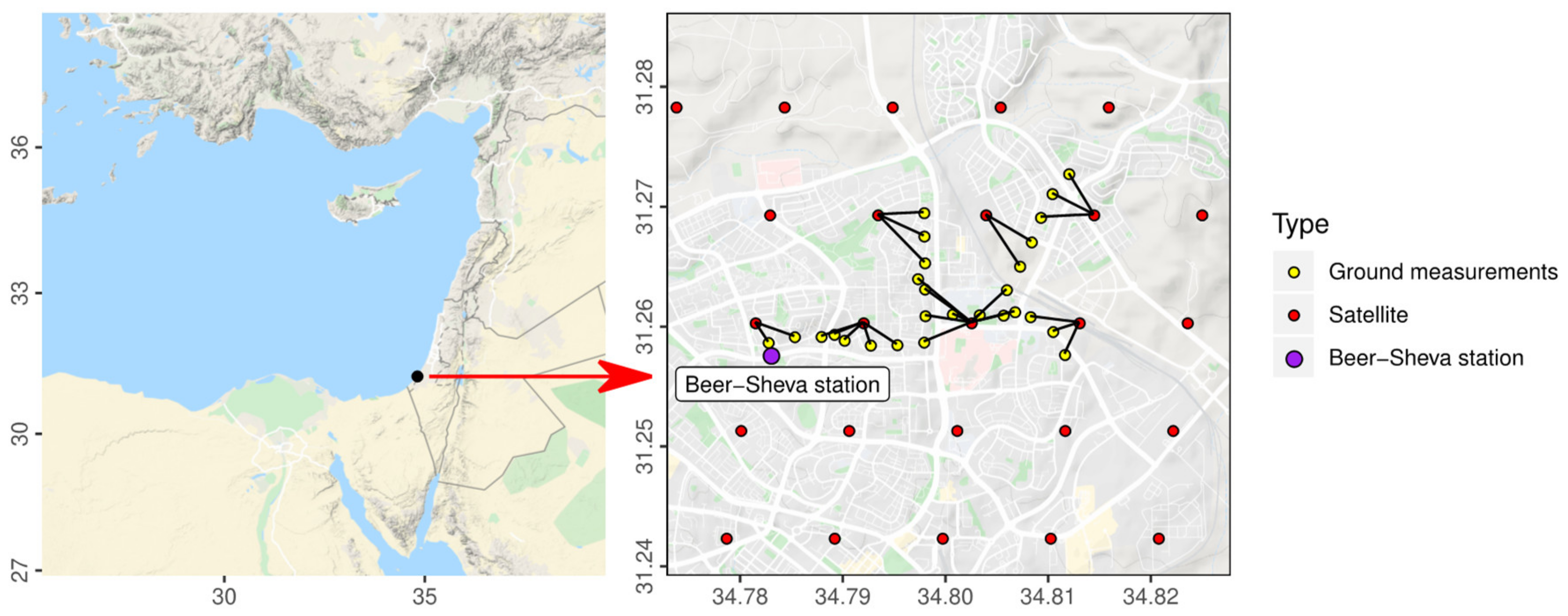
2.1. Study Area
2.2. Environmental Data
2.3. Hardware
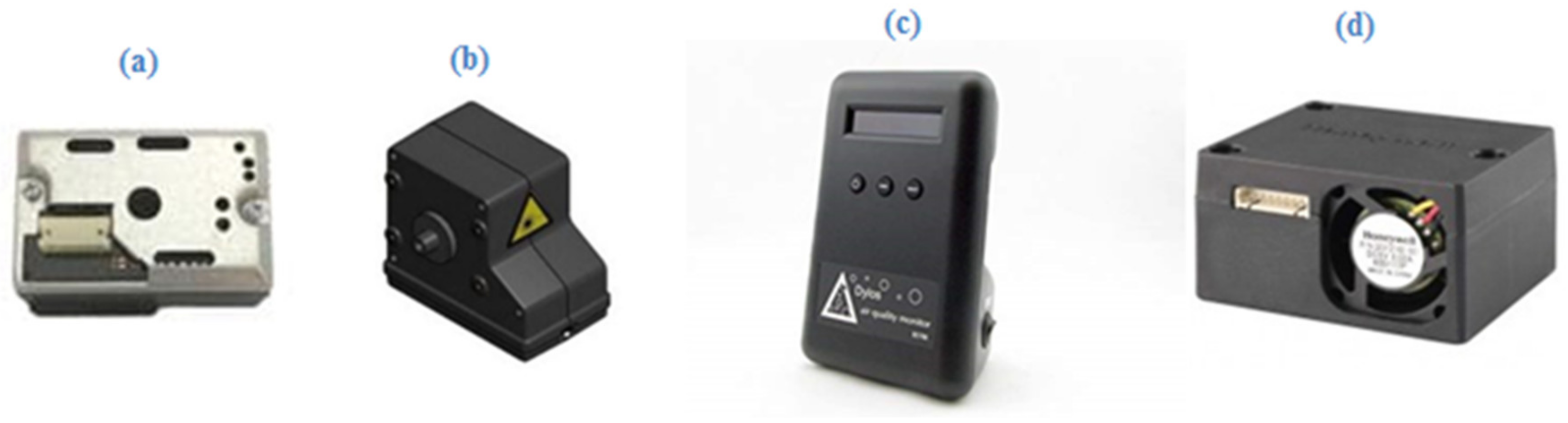
2.3.1. COTS Sensors
2.3.2. Kit Development
2.4. PM Measurements
2.4.1. Measurements under Laboratory Conditions
2.4.2. Preliminary Outdoor Testing
2.4.3. Comparison with TEOM Data
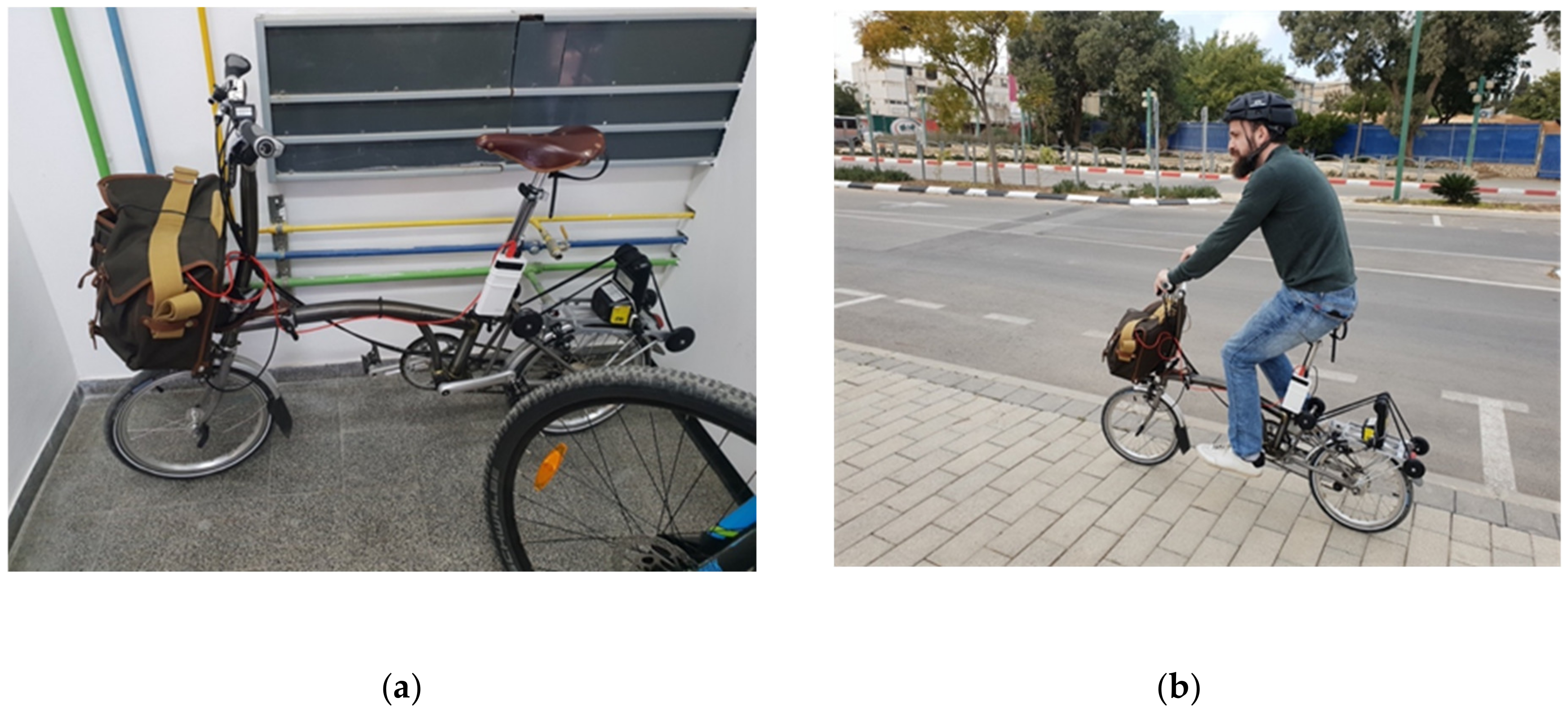
2.4.4. Mobile Measurement Campaign by Bicycle
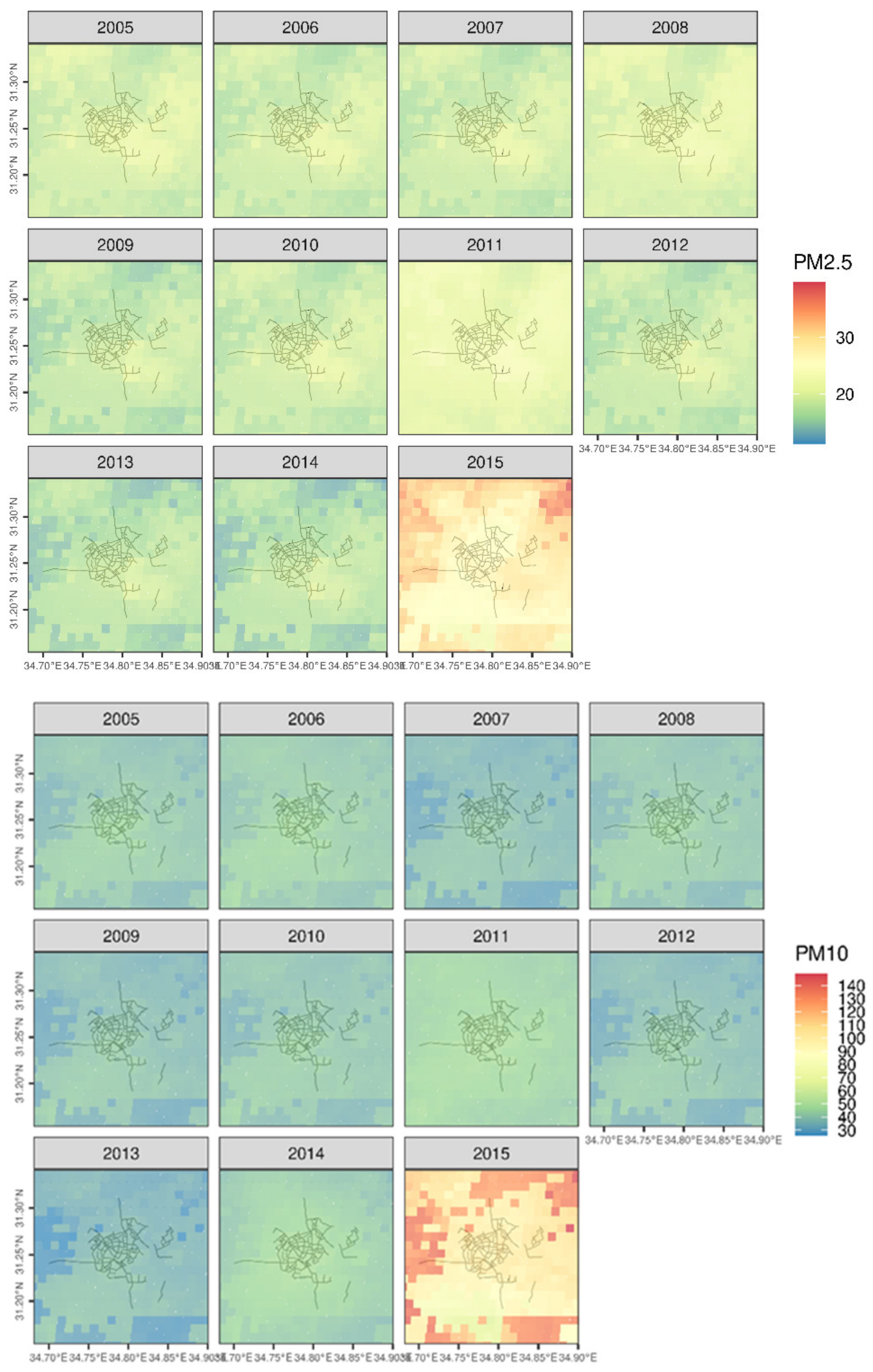
2.4.5. Satellite Based PM Models
2.4.6. Data Structuring and Interpolation
- Linear regression of COTS sensor PM as a function of TEOM PM
- Linear regression of COTS sensor PM as a function of TEOM PM and four meteorological variables (temperature, relative humidity, wind speed and wind direction)
- A random forests model of COTS sensor PM as a function of TEOM PM and the abovementioned four meteorological variables. The random forest framework was used given that its highly equipped to deal with non-linear relationships, since decision tree models in general, and random forest specifically, are able to choose by which features to split the data, with no limitation on the amount of splits. It can create a decision boundary, which is complex and non-linear.
3. Results
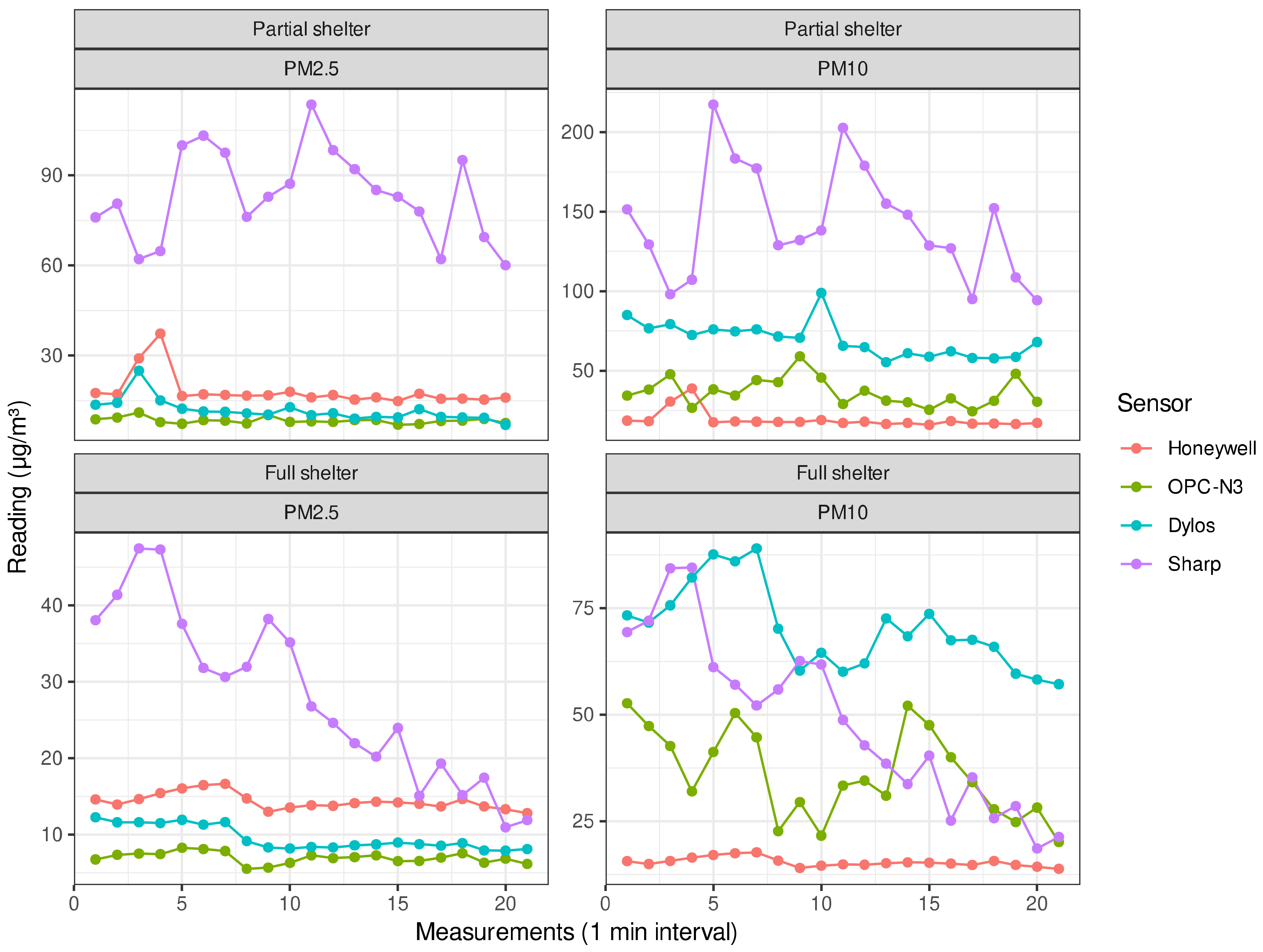
3.1. Lab Tests
3.2. Outdoor Tests
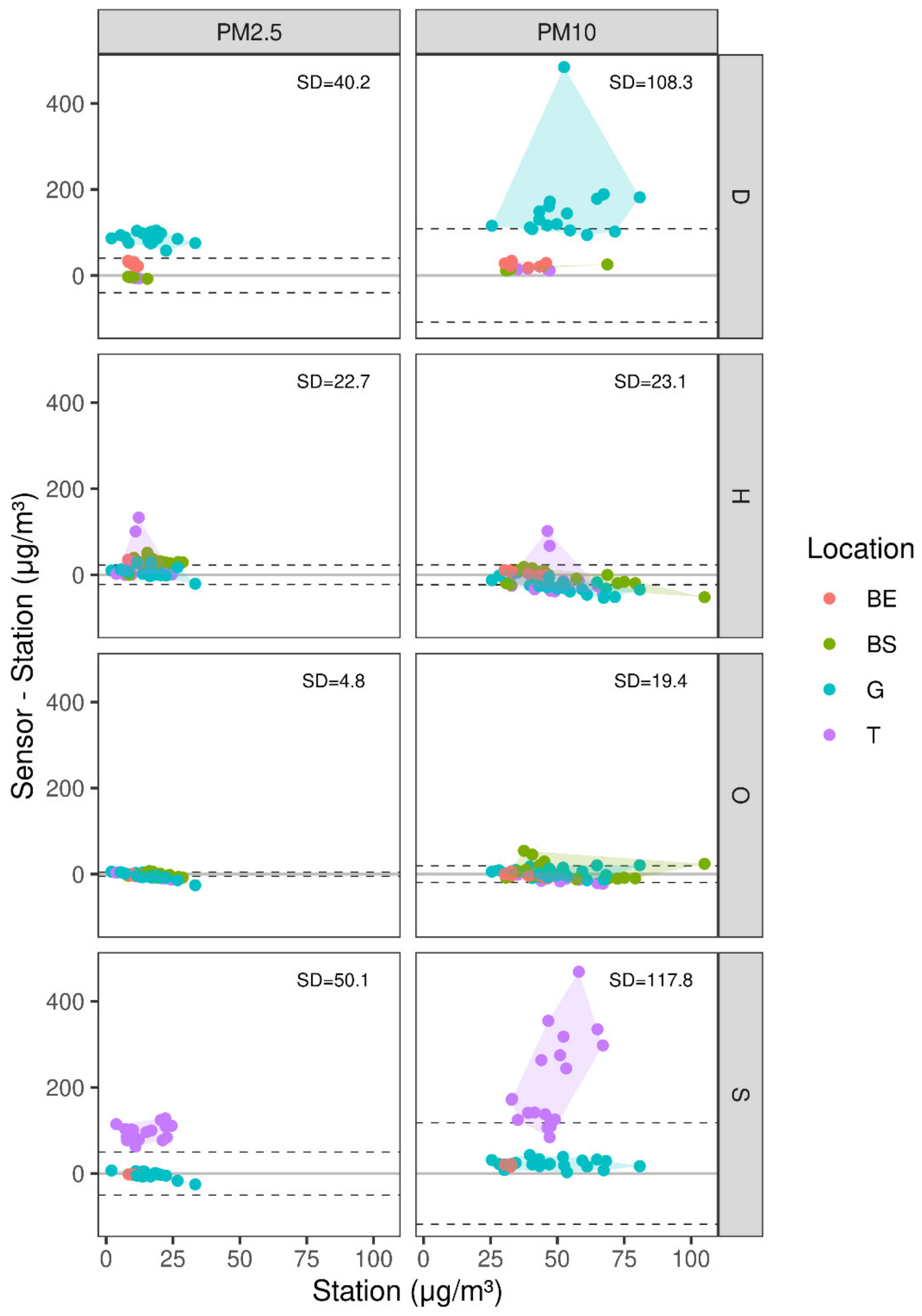
3.3. Comparison with TEOM
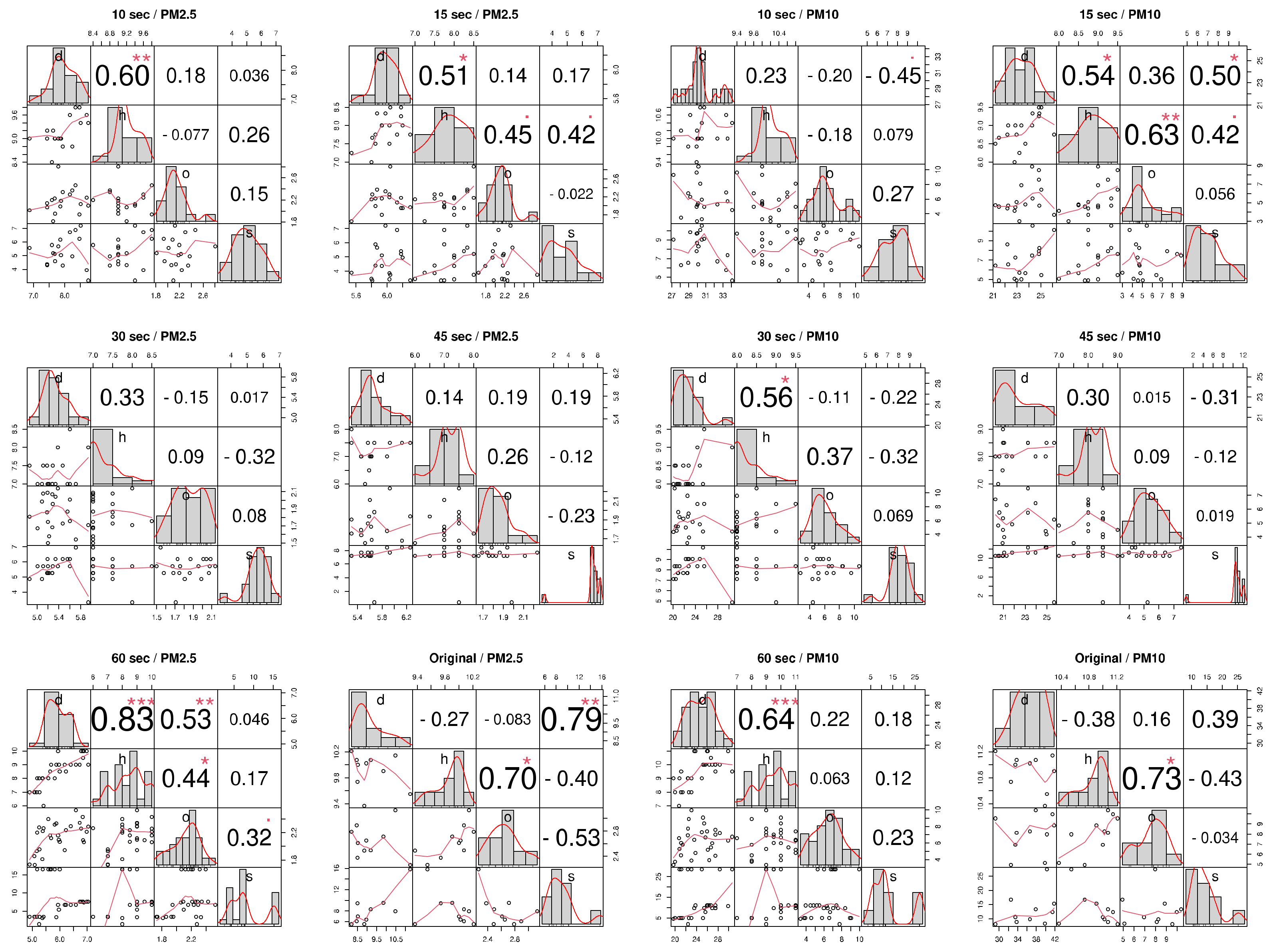
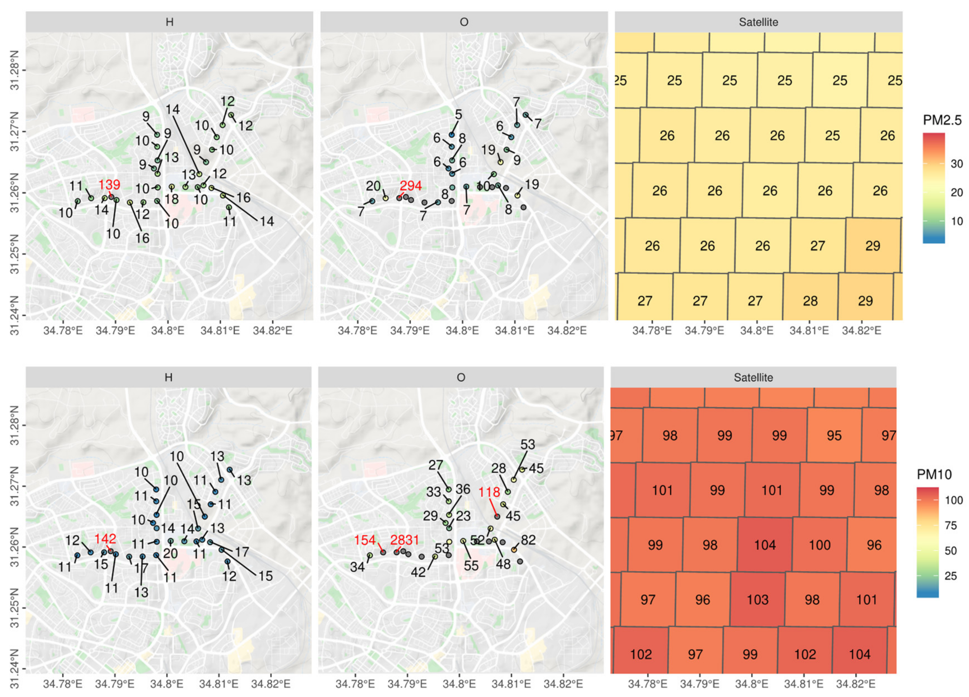
3.4. Mobile Measurement Campaign
4. Discussion
5. Conclusions
Author Contributions
Funding
Conflicts of Interest
Appendix A

| Variable | Model | Slope | Intercept | R2 |
|---|---|---|---|---|
| Honeywell-PM2.5 | Linear model—TEOM | 30.6388 | −0.011 | −0.022722584 |
| Honeywell-PM2.5 | Linear model: TEOM + Meteorological factors | 27.9802 | 0.0552 | −0.001513723 |
| Honeywell-PM2.5 | Random Forests: TEOM + Meteorological factors | 28.46 | 0.0968 | 0.161438272 |
| Honeywell-PM10 | Linear model: TEOM | 32.4745 | −0.0534 | 0.019061521 |
| Honeywell-PM10 | Linear model: TEOM + Meteorological factors | 29.133 | 0.0436 | −0.028409946 |
| Honeywell-PM10 | Random Forests: TEOM + Meteorological factors | 32.4729 | 0.0417 | −0.008819204 |
| OPC-N3-PM2.5 | Linear model: TEOM | 6.7076 | 0.3038 | 0.483495144 |
| OPC-N3-PM2.5 | Linear model: TEOM + Meteorological factors | 2.6469 | 0.7821 | 0.57609834 |
| OPC-N3-PM2.5 | Random Forests: TEOM + Meteorological factors | 6.1345 | 0.3937 | 0.554083995 |
| OPC-N3-PM10 | Linear model: TEOM | 24.7203 | 0.4026 | 0.581336121 |
| OPC-N3-PM10 | Linear model: TEOM + Meteorological factors | 25.6637 | 0.3808 | 0.589789448 |
| OPC-N3-PM10 | Random Forests: TEOM + Meteorological factors | 34.1448 | 0.194 | 0.362786724 |
| Sharp-PM2.5 | Linear model: TEOM | 54.9663 | 0.0014 | −0.048504135 |
| Sharp-PM2.5 | Linear model: TEOM + Meteorological factors | 64.0294 | 0.3702 | 0.124500294 |
| Sharp-PM2.5 | Random Forests: TEOM + Meteorological factors | 50.3221 | 0.276 | 0.325243306 |
| Sharp-PM10 | Linear model: TEOM | 126.2785 | 0.055 | 0.191369713 |
| Sharp-PM10 | Linear model: TEOM + Meteorological factors | 159.4208 | 0.189 | 0.104123008 |
| Sharp-PM10 | Random Forests: TEOM + Meteorological factors | 131.6534 | 0.1987 | 0.422302067 |
| Dylos-PM2.5 | Linear model: TEOM | 52.8526 | 0.2487 | 0.140869256 |
| Dylos-PM2.5 | Linear model: TEOM + Meteorological factors | 12.6777 | 0.9736 | 0.858485926 |
| Dylos-PM2.5 | Random Forests: TEOM + Meteorological factors | 43.0559 | 0.2858 | 0.384341244 |
| Dylos-PM10 | Linear model: TEOM | 97.8045 | 0.4519 | 0.390104326 |
| Dylos-PM10 | Linear model: TEOM + Meteorological factors | 5.205 | 1.2015 | 0.828236601 |
| Dylos-PM10 | Random Forests: TEOM + Meteorological factors | 103.1206 | 0.2891 | 0.661054684 |
References
- Itai, K.; Steven, J.M.; William, L.R.; Brent, A.C.; Joel, S. Using new satellite based exposure methods to study the assosication between pregnancy pm2.5 exposure, premature birth and birth weight in Massachusetts. Environ. Health 2012, 11, 40. [Google Scholar]
- Luisa, M. Contribution of Natural Sources to Air Pollution Levels in the EU—A Technical Basis for the Development of Guidance for the Member States; EUR—Scientific and Technical Research Reports: Ispra, Italy, 2007. [Google Scholar]
- Francisco, P.; Ioana, I. Anthropogenic Air Pollution Sources. Air Qual. 2010. [Google Scholar] [CrossRef]
- Helena, K.; Itzhak, K.; Petros, K.; Michael, D. Friger. Contribution of dust storms to PM10 levels in urban arid environments. J. Air Waste Manag. Assos. 2014, 64, 89–94. [Google Scholar]
- Eliezer, G.; Isabella, O.; Amnon, S.; Pinhas, A. Increasing trend of African dust, over 49 year, in the eastern Mediterranean. JGR Atmos. 2010, 115, D7. [Google Scholar] [CrossRef]
- Krasnov, H.; Katra, I.; Friger, M. Increase in dust storm related PM10 concentrations: A time series analysis of 2001–2015. Environ. Pollut. 2016, 213, 36–42. [Google Scholar] [CrossRef]
- US Burden of Disease Collaborators. The State of US Health, 1990–2010: Burden of Diseases, Injuries, and Risk Factors. JAMA 2013, 310, 591–606. [Google Scholar] [CrossRef]
- World Health Organization. The World Health Report-Reducing Risks, Promoting Healithy Life; WHO: Geneva, Switzerland, 2002. [Google Scholar]
- D’Ippoliti, D.; Forastiere, F.; Ancona, C.; Agabiti, N.; Fusco, D.; Michelozzi, P.; Perucci, C.A. Air pollution and myocardial infarction in Rome: A case-crossover analysis. Epidemiology 2003, 14, 528–535. [Google Scholar] [CrossRef]
- Hodas, N.; Turpin, B.; Lunden, M. Refined ambient PM2.5 exposure surrogates and the risk of myocardial infarction. J. Expo. Sci. Environ. Epidemiol. 2013, 23, 578–580. [Google Scholar] [CrossRef]
- Jaime, M.; Itai, K.; Robert, G.; Brent, A.C.; Murray, A.; Mittleman, J.S. Long-term Exposure to PM2.5 and incidence of Acute Myocardial Infarction. Environ. Health Perspect. 2013, 121, 2. [Google Scholar] [CrossRef]
- Rich, D.Q. The Triggering of Myocardial Infarction by Fine Partifles is Enhanced When Particles Are Enriched in Secondary Species. Environ. Sci. Technol. 2013, 47, 9414–9423. [Google Scholar] [CrossRef]
- O’Neil, M.S.; Veves, A.; Zanobetti, A.; Sarnat, J.A.; Gold, D.R.; Economides, P.A.; Horton, E.S.; Schwartz, J. Diabetes Enhances Vulnerability to Particulate Air Pollution-Associated Impairment in Vascular Reactivity and Endothelial Function. Circulation 2015, 111, 22. [Google Scholar] [CrossRef]
- Zeka, A.; Schwartz, J.; Melly, S.J. Traffic-Related and Socioeconomic Indications in Association With Low Birth Weight and Preterm Births in Eastern Massachusetts Between 1996–2002. Epidemiology 2006, 17, 105. [Google Scholar] [CrossRef][Green Version]
- Bell, M.L.; Ebisu, K.; Belanger, K. Ambient Air Pollution and Low Birth Weight in Connecticut and Massachusetts. Environ. Health Perspect. 2007, 115, 7. [Google Scholar] [CrossRef]
- Dominici, F.; Peng, R.D.; Bell, M.L. Fine Particulate Air Pollution and Hospital Admission for Cardiovascular and Respiratory Diseases. JAMA 2006, 295, 1127–1134. [Google Scholar] [CrossRef]
- Angela, I.-M.; Kirsi, L.; Timonen, A.P.; Joachim, H.; Gbriele, W.; Timo, L.; Gintautas, B.; Wolfgang, G.; Kreyling, J.D.H.; Gerard, H.; et al. Effects of Particulate air pollution on blood pressure and heart rate in subjects with cardiovascular disease: A multicenter approach. Environ. Health Perspect. 2004. [Google Scholar] [CrossRef]
- Mann, J.K. Air pollution and hospital admissions for ischemic heart disease in persons with congestive heart failure or arrhythmia. Environ. Health Perspect. 2002, 110, 1247. [Google Scholar] [CrossRef]
- Crouse, D.L.; Peters, P.A.; Van Donkelaar, A.; Goldberg, M.S.; Villeneuve, P.J.; Brion, O.; Khan, S.; Atari, D.O.; Jerrett, M.; Pope, C.A.; et al. Risk of Nonaccidental and Cadiovascular Mortality in Relation to Long-term Exposure to Low Concentrations of Fine Particulate Matter: A Canadian National-Level Cohort Study. Environ. Health Perspect. 2012, 120, 5. [Google Scholar] [CrossRef]
- Joel, S. Air Pollution and Hospital Admissions for Cardiovascular Disease in Tuscon. Epidemiology 1997, 8, 371–377. [Google Scholar]
- Khaniabadi, Y.O.; Fanelli, R.; De Marco, A. Hospital admissions in Iran for cardiovascular and respiratory diseases attributed to the Middle Eastern Dust storms. Environ. Sci. Pollut. Res. 2017, 24, 16860–16868. [Google Scholar] [CrossRef]
- Kloog, I.; Ridgway, B.; Koutrakis, P.; Coull, B.A.; Schwartz, J.D. Long and Short Term Exposure to PM2.5 and Mortality. Epidemiology 2013, 24, 555–561. [Google Scholar] [CrossRef]
- Joel, S. Air pollution and Hospital Admissions for Respiratory Disease. Epidemiology 1996, 7, 20–28. [Google Scholar]
- Butt, E.W.; Turnock, S.T. Global and regional trends in particulate air pollution and attributable health burden over the past 50 years. Environ. Res. Lett. 2017, 12, 10. [Google Scholar] [CrossRef]
- Zeger, S.L.; Thomas, D.; Dominici, F.; Samet, J.M.; Schwartz, J.; Dockery, D.; Cohen, A. Exposure measurement error in time-series studies of air pollution: Concepts and consequences. Environ Health Perspect. 2000, 10, 419–426. [Google Scholar] [CrossRef] [PubMed]
- Kloog, I.; Sorek-Hamer, M.; Lyapustin, A.; Coull, B.; Wang, Y.; Just, A.C.; Schwartz, J.; Broday, D.M. Estimating daily PM2.5 and PM10 across the complex geo-climate region of Israel using MAIAC satellite-based AOD data. Atmos. Environ. 2015, 122, 409–416. [Google Scholar] [CrossRef] [PubMed]
- Jovanovic, U.Z.; Jovanovic, I.D.; Petrusic, A.Z.; Petrusic, Z.M.; Mančić, D.D. Low-cost wireless dust monitoring system. In Proceedings of the 11th International Conference on Telecommunications in Modern Satellite, Cable and Broadcasting Services, Nis, Serbia, 16–19 October 2013; pp. 635–638. [Google Scholar] [CrossRef]
- Farukh, S. Satellite monitoring of wireless sensor networks. Procedia Comput. Sci. 2013, 21, 479–484. [Google Scholar]
- Budde, M.; El Masri, R.; Riedel, T.; Beigl, M. Enabling Low-Cost Particulate Matter Measurement for Participatory Sensing Scenarios. In Proceedings of the 12th International Conference on Mobile and Ubiquitous Multimedia, Lulea, Sweden, 2–5 December 2013; pp. 1–10. [Google Scholar]
- Yu, X.; Shi, Y.; Wang, T.; Sun, X. Dust-concentration measurement based on Mie scattering of a laser beam. PLoS ONE 2017, 12, 8. [Google Scholar] [CrossRef] [PubMed]
- Krasnov, H.; Kloog, I.; Friger, M.; Katra, I. The Spatio-Temporal Distribution of Particulate Matter during Natural Dust Episodes at an Urban Scale. PLoS ONE 2016, 11, 8. [Google Scholar] [CrossRef] [PubMed]
- Mokhloss, I.; Khadem, V.S. Dust Monitoring Systems. The Sixth International Conference on Systems and Networks Communications. 2011. Available online: http://citeseerx.ist.psu.edu/viewdoc/download?doi=10.1.1.1001.9709&rep=rep1&type=pdf (accessed on 25 February 2019).
- Ashish, M.; Husain, T.H.R.; Haque, M.I.; Rakibul, A. Air Quality Monitoring: The use of Arduino and Android. J. Mod. Sci. Technol. 2016, 4, 86–96. [Google Scholar]
- Elen, B.; Peters, J.; Van Poppel, M.; Bleux, N.; Theunis, J.; Reggente, M.; Standaert, A. The Aeroflex: A Bicycle for Mobile Air Quality Measurements. Sensors 2012, 13, 221–240. [Google Scholar] [CrossRef]
- Kuznetsov, S.; Paulos, E. Participatory sensing in public spaces: Activating urban surfaces with sensor probes. In Proceedings of the 8th ACM conference on Designing Interactive Systems, Aarhus, Denmark, 16–20 August 2010; pp. 21–30. [Google Scholar] [CrossRef]
- Aicardi, I.; Gandino, F.; Grasso, N.; Lingua, A.M.; Noardo, F. A Low-Cost Solution for the Monitoring of Air Pollution Parameters through Bicycles. Intern. Conf. Comput. Sci. Appl. 2017, 10407, 105–120. [Google Scholar]
- Liu, X.; Xiang, C.; Li, B.; Jiang, A. Collaborative Bicycle Sensing for Air Pollution on Roadway. In Proceedings of the 12th International Conference on Ubiquitous Intelligence and Computing, Beijing, China, 10–14 August 2015; pp. 316–319. [Google Scholar] [CrossRef]
- Dylos AQ-SPEC Handbook. Available online: http://www.dylosproducts.com/dc1700.html (accessed on 27 February 2019).
- Wang, R.; Fei, T.; Wang, L.; Zhou, Z. Design of high precision PM2.5 detector based on laser sensor. In Proceedings of the IEEE 8th Joint International Information Technology and Artificial Intelligence Conference, Chongqing, China, 24–26 May 2019; pp. 1130–1133. [Google Scholar] [CrossRef]
- Hojaiji, H.; Kalantarian, H.; Bui, A.A.T.; King, C.E.; Sarrafzadeh, M. Sarrafzadeh. Temperature and humidity calibration of low cost wireless dust sensor for real time monitoring. IEEE Sens. Appl. Symp. 2017, 1–6. [Google Scholar] [CrossRef]
- Jones, S.; Anthony, T.R.; Sousan, S.; Altmaier, R.; Park, J.H.; Peters, T.M. Evaluation of a Low Cost Aerosol Sensor to Assess Dust Concentration in a Swine Building. Ann. Occup. Hyg. 2016, 60, 597–607. [Google Scholar] [CrossRef] [PubMed]
- Sharp-GP2Y1030AU0F Dust Sensor Data Sheet. Available online: http://global.sharp/products/device/lineup/selection/pdf/opto_dms201809_e.pdf (accessed on 14 August 2019).
- Yang, Y.; Russel, L.; Lou, S. Dust-wind interactions can intensify aerosol pollution over eastern China. Nat. Commun. 2017, 8, 15333. [Google Scholar] [CrossRef] [PubMed]
- Shtein, A.; Karnieli, A.; Katra, I.; Raz, R.; Levy, I.; Lyapustin, A.; Dorman, M.; Broday, D.M.; Kloog, I. Estimating daily and intra-daily PM10 and PM2.5 in Israel using a spatio-temporal hybrid modeling approach. Atmos. Environ. 2018, 191. [Google Scholar] [CrossRef]
- Arvani, B.; Pierce, R.B.; Lyapustin, A.I.; Wang, Y.; Ghermandi, G.; Teggi, S. Seasonal monitoring and estimation of regional aerosol distribution over Po valley, northern Italy, using a high-resolution MAIAC product. Atmos. Environ. 2016, 141, 106–121. [Google Scholar] [CrossRef]
- De Hoogh, K.; Chen, J.; Gulliver, J.; Hoffmann, B.; Hertel, O.; Ketzel, M.; Klompmaker, J. Spatial PM2.5, NO2, O3 and BC models for Western Europe–Evaluation of spatiotemporal stability. Environ. Int. 2018, 120, 81–92. [Google Scholar] [CrossRef]
- Just, A.C.; Wright, R.O.; Schwartz, J.; Coull, B.A.; Baccarelli, A.A.; Tellez-Rojo, M.M.; Kloog, I. Using high-resolution satellite aerosol optical depth to estimate daily PM2.5 geographical distribution in Mexico City. Environ. Sci. Technol. 2015, 49, 8576–8584. [Google Scholar] [CrossRef]
- Stafoggia, M.; Schwartz, J.; Badaloni, C.; Bellander, T.; Alessandrini, E.; Cattani, G.; Sorek-Hamer, M. Estimation of daily PM10 concentrations in Italy (2006–2012) using finely resolved satellite data, land use variables and meteorology. Environ. Int. 2017, 99, 234–244. [Google Scholar] [CrossRef]
- Zhang, H.; Lyapustin, A.; Wang, Y.; Kondragunta, S.; Laszlo, I.; Ciren, P.; Hoff, R.M. A multi-angle aerosol optical depth retrieval algorithm for geostationary satellite data over the United States. Atmos. Chem. Phys. 2011, 11. [Google Scholar] [CrossRef]
- Sorek-Hamer, M.; Stupp, A.; Alpert, P.; Broday, D.M. Characteristics of the east Mediterranean dust variability on small spatial and temporal scales. Atmos. Environ. 2015, 120, 51–60. [Google Scholar] [CrossRef]
- Olivardes, G.; Edwards, S. The Outdoor Dust Information Node (ODIN)–development and performance assessment of a low cost ambient dust sensor. Atmos. Meas. Tech. Discuss. 2015, 8, 7511–7533. [Google Scholar] [CrossRef]
- Bulot, F.M.J.; Johnstom, S.J.; Basford, P.J. Long-term field comparison of multiple low-cost particulate matter sensors in an outdoor urban environment. Sci. Rep. 2019, 9, 7497. [Google Scholar] [CrossRef]
- Budde, M.; Schwarz, A.D.; Müller, T.; Laquai, B.; Streibl, N.; Schindler, G.; Beigl, M. Potential and limitations of the low-cost SDS011 particle sensor for monitoring urban air quality. ProScience 2018, 5, 6–12. [Google Scholar]
- Badura, M.; Batog, P.; Drzeniecka-Osiadacz, A.; Modzel, P. Evaluation of low-cost sensors for ambient PM2.5 monitoring. J. Sens. 2018, 2018, 5096540. [Google Scholar] [CrossRef]
- Budde, M.; Müller, T.; Laquai, B.; Streibl, N.; Schwarz, A.; Schindler, G.; Dittler, A. Suitability of the Low-Cost SDS011 Particle Sensor for Urban PM-Monitoring. Sci. Res. Abstr. 2018, 8, 11. [Google Scholar]
- Malings, C.; Tanzer, R.; Hauryliuk, A.; Saha, P.K.; Robinson, A.L.; Presto, A.A.; Subramanian, R. Fine particle mass monitoring with low-cost sensors: Corrections and long-term performance evaluation. Aerosol Sci. Technol. 2020, 54, 160–174. [Google Scholar] [CrossRef]
- Kelly, K.E.; Whitaker, J.; Petty, A.; Widmer, C.; Dybwad, A.; Sleeth, D.; Butterfield, A. Ambient and laboratory evaluation of a low-cost particulate matter sensor. Environ. Pollut. 2017, 221, 491–500. [Google Scholar] [CrossRef]
- Sayahi, T.; Butterfield, A.; Kelly, K.E. Long-term field evaluation of the Plantower PMS low-cost particulate matter sensors. Environ. Pollut. 2019, 245, 932–940. [Google Scholar] [CrossRef]
- Wang, Y.; Li, J.; Jing, H.; Zhang, Q.; Jiang, J.; Biswas, P. Laboratory evaluation and calibration of three low-cost particle sensors for particulate matter measurement. Aerosol Sci. Technol. 2015, 49, 1063–1077. [Google Scholar] [CrossRef]
- Gupta, P.; Doraiswamy, P.; Levy, R.; Pikelnaya, O.; Maibach, J.; Feenstra, B.; Mills, K.C. Impact of California fires on local and regional air quality: The role of a low-cost sensor network and satellite observations. GeoHealth 2018, 2, 172–181. [Google Scholar] [CrossRef]
- Bi, J.; Stowell, J.; Seto, E.Y.; English, P.B.; Al-Hamdan, M.Z.; Kinney, P.L.; Liu, Y. Contribution of low-cost sensor measurements to the prediction of PM2.5 levels: A case study in Imperial County, California, USA. Environ. Res. 2020, 180, 108810. [Google Scholar] [CrossRef] [PubMed]
- Isaifan, R.J. The dramatic impact of Coronavirus outbreak on air quality: Has it saved as much as it has killed so far? Glob. J. Environ. Sci. Manag. 2020, 6, 275–288. [Google Scholar]


| COTS Sensor (Manufacturer) | Sharp-GP2Y1030AU0F | Alphanese-OPC-N3 | Honeywell-HPMA115S0-XXX | Dylos-DC1700 |
|---|---|---|---|---|
| Method | An infrared emitting diode and a phototransistor are diagonally arranged into this device, to allow it to detect the reflected light of dust in air. | OPCs provide digital outputs of PM1, PM2.5 and PM10 every second, along with histograms of the particle count for each size. Device’s flow correction improves stable readings, even in high dust environments. | utilizes a laser-based light scattering particle sensing method to detect particulates from 0.3 μm to 5 μm | Counts individual particles, gives immediate response to change in environment and provides three different history modes; minute, hour and day, up to 30 days of stored history data. |
| Range | 0–500 μg/m3 | 0–2000 μg/m3 | 0–1000 μg/m3 | Unspecified |
| Price | $12 | $250 | $25 | $450 |
Publisher’s Note: MDPI stays neutral with regard to jurisdictional claims in published maps and institutional affiliations. |
© 2020 by the authors. Licensee MDPI, Basel, Switzerland. This article is an open access article distributed under the terms and conditions of the Creative Commons Attribution (CC BY) license (http://creativecommons.org/licenses/by/4.0/).
Share and Cite
Lesser, D.; Katra, I.; Dorman, M.; Harari, H.; Kloog, I. Validating and Comparing Highly Resolved Commercial “Off the Shelf” PM Monitoring Sensors with Satellite Based Hybrid Models, for Improved Environmental Exposure Assessment. Sensors 2021, 21, 63. https://doi.org/10.3390/s21010063
Lesser D, Katra I, Dorman M, Harari H, Kloog I. Validating and Comparing Highly Resolved Commercial “Off the Shelf” PM Monitoring Sensors with Satellite Based Hybrid Models, for Improved Environmental Exposure Assessment. Sensors. 2021; 21(1):63. https://doi.org/10.3390/s21010063
Chicago/Turabian StyleLesser, Dan, Itzhak Katra, Michael Dorman, Homero Harari, and Itai Kloog. 2021. "Validating and Comparing Highly Resolved Commercial “Off the Shelf” PM Monitoring Sensors with Satellite Based Hybrid Models, for Improved Environmental Exposure Assessment" Sensors 21, no. 1: 63. https://doi.org/10.3390/s21010063
APA StyleLesser, D., Katra, I., Dorman, M., Harari, H., & Kloog, I. (2021). Validating and Comparing Highly Resolved Commercial “Off the Shelf” PM Monitoring Sensors with Satellite Based Hybrid Models, for Improved Environmental Exposure Assessment. Sensors, 21(1), 63. https://doi.org/10.3390/s21010063