A Contactless Laser Doppler Strain Sensor for Fatigue Testing with Resonance-Testing Machine

Abstract
1. Introduction
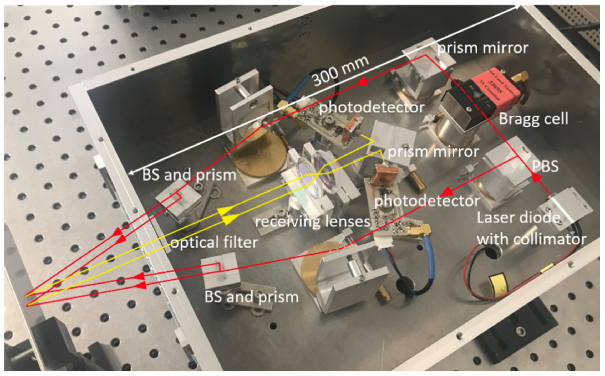
2. Optical Setup
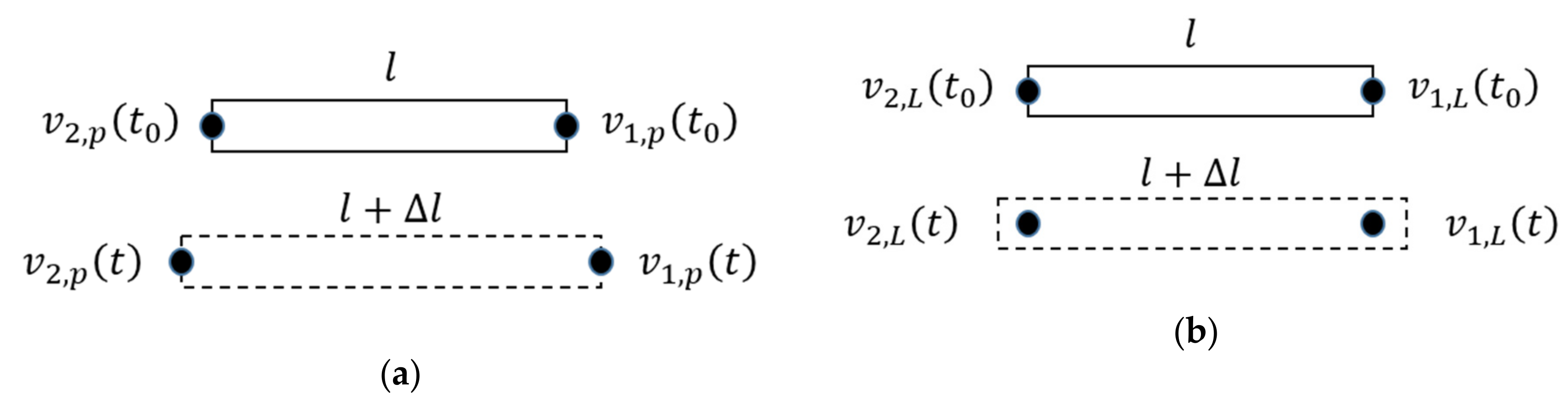
3. Modeling
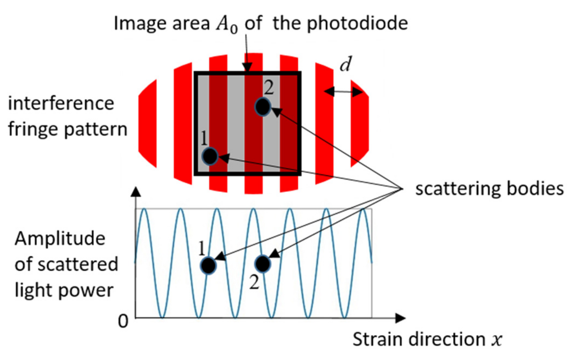
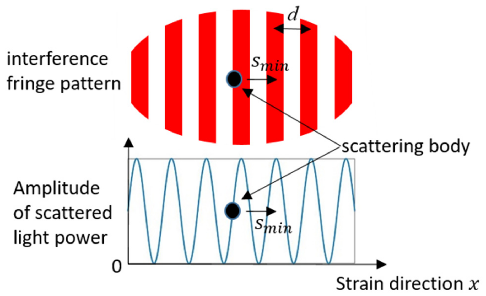
3.1. Signal Power
3.2. Noise Analysis and SNR
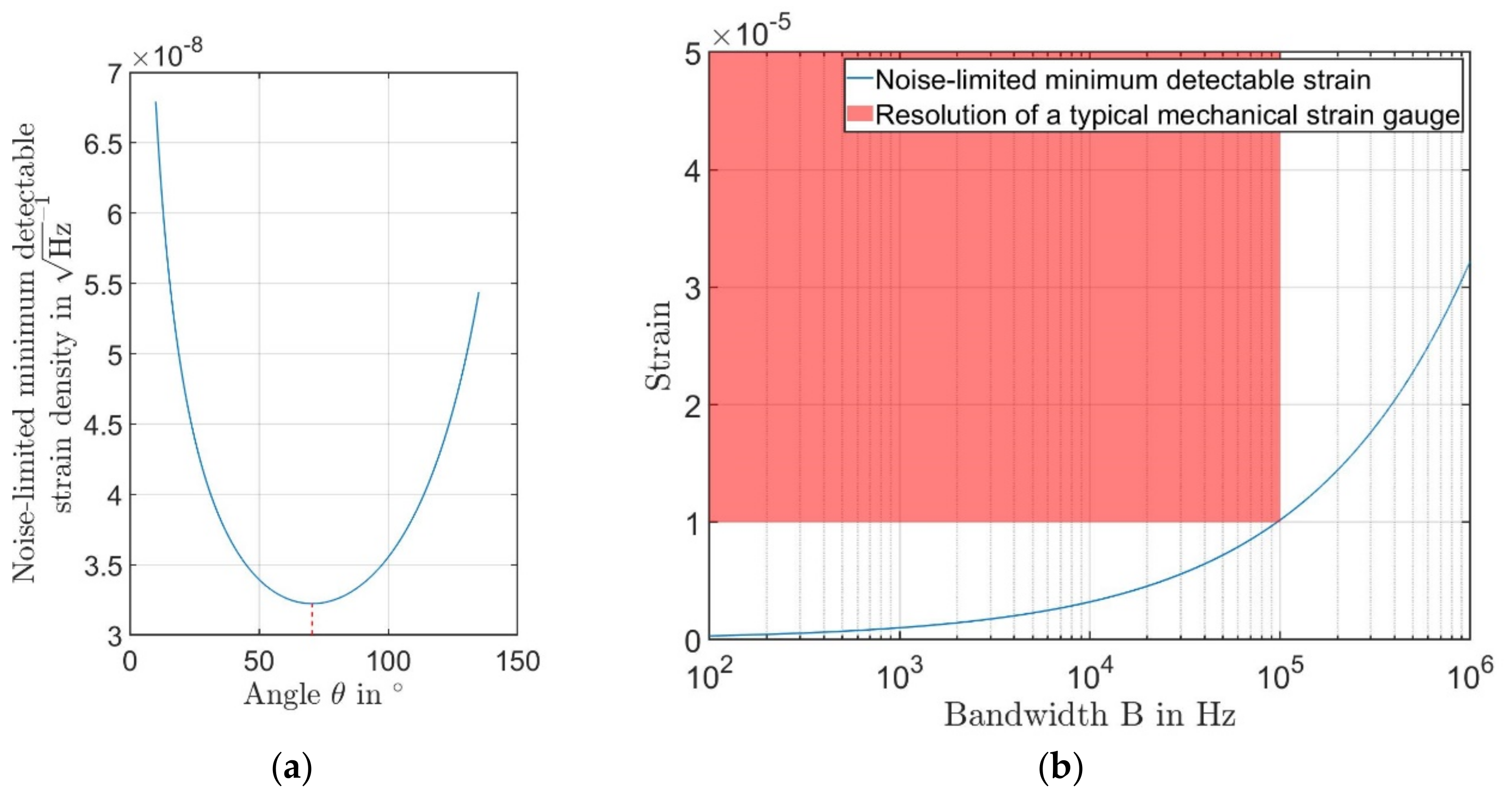
3.3. Noise Limited Resolution
3.4. Simulation for the Optimal Sensor Design
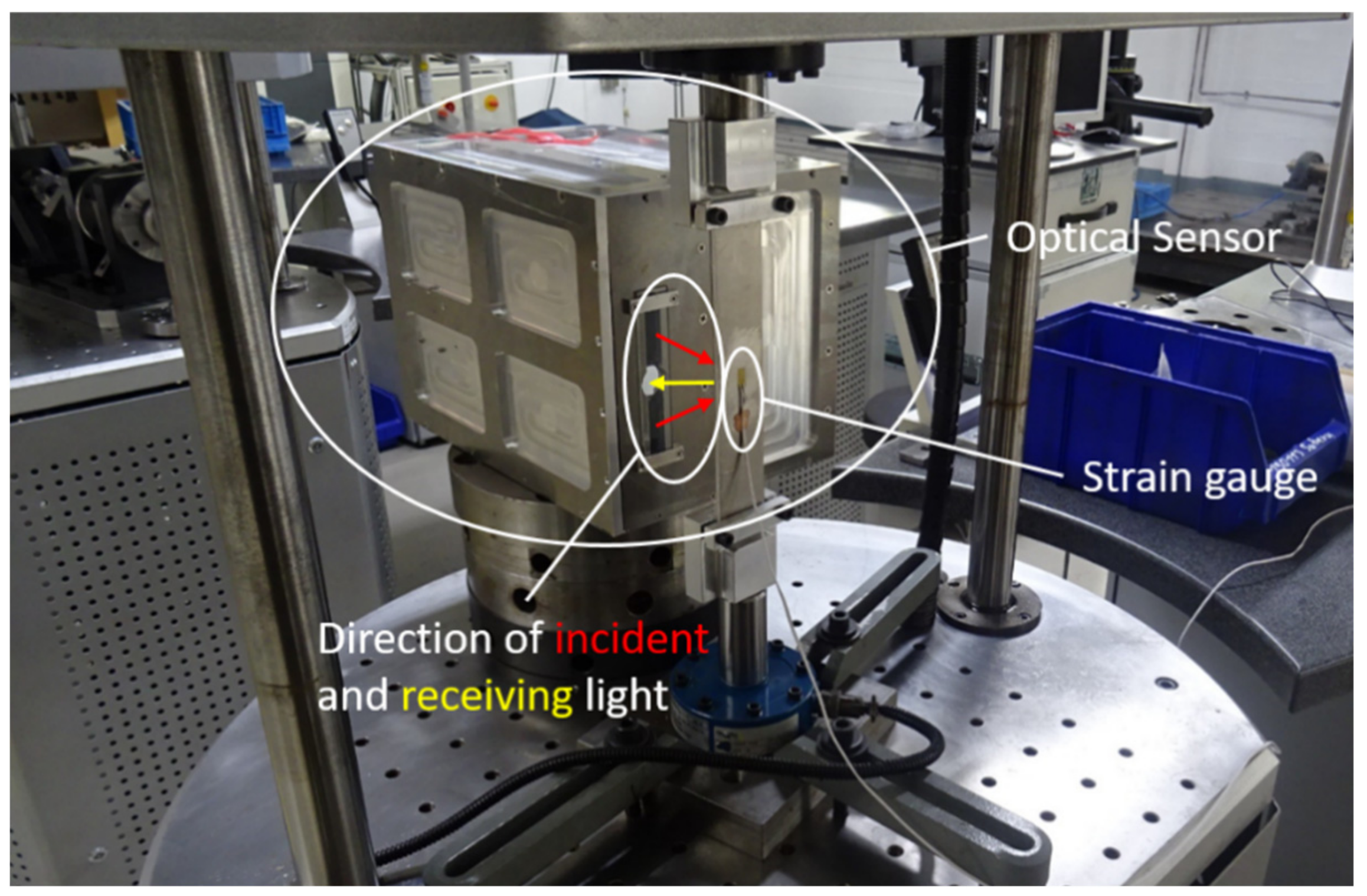
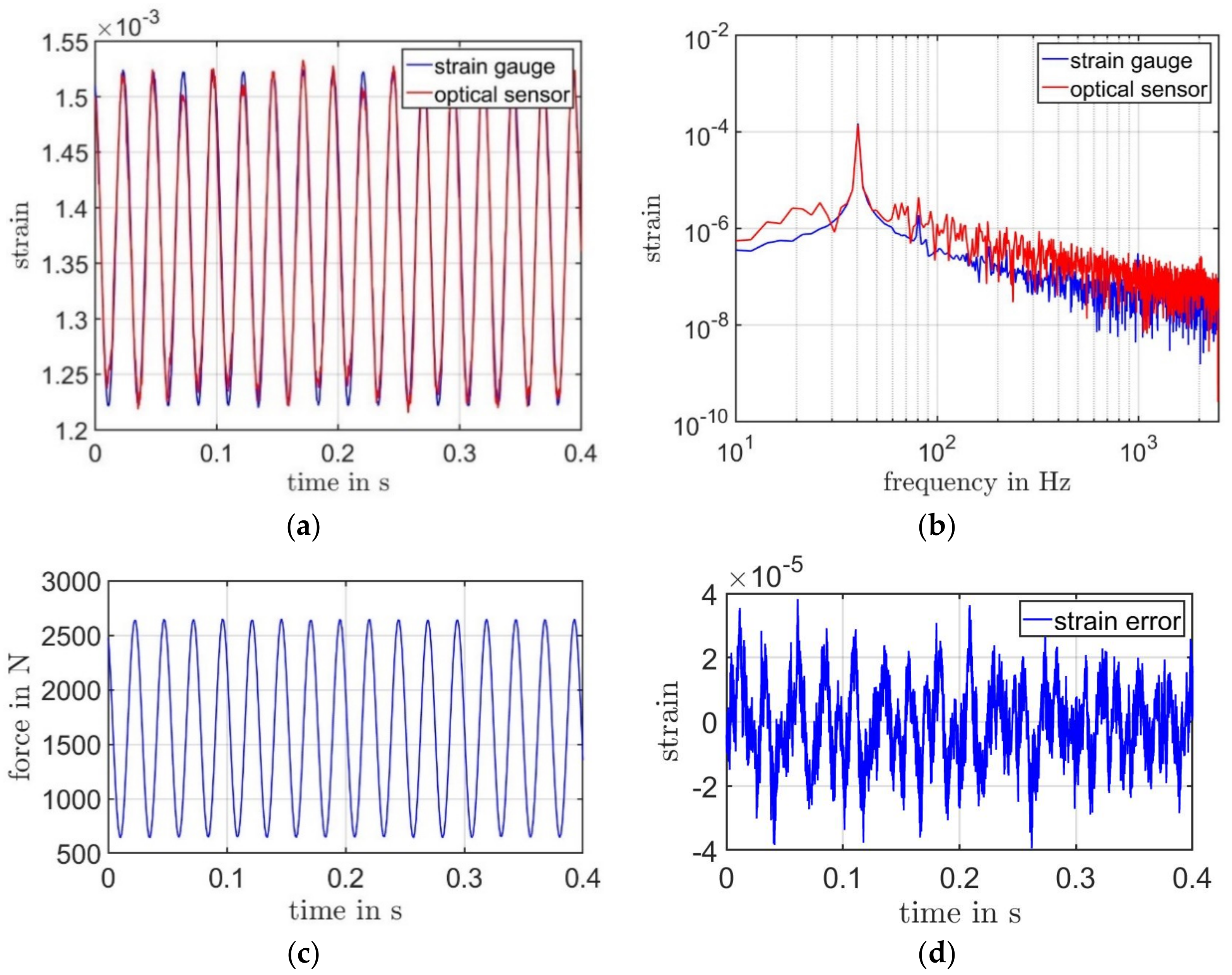
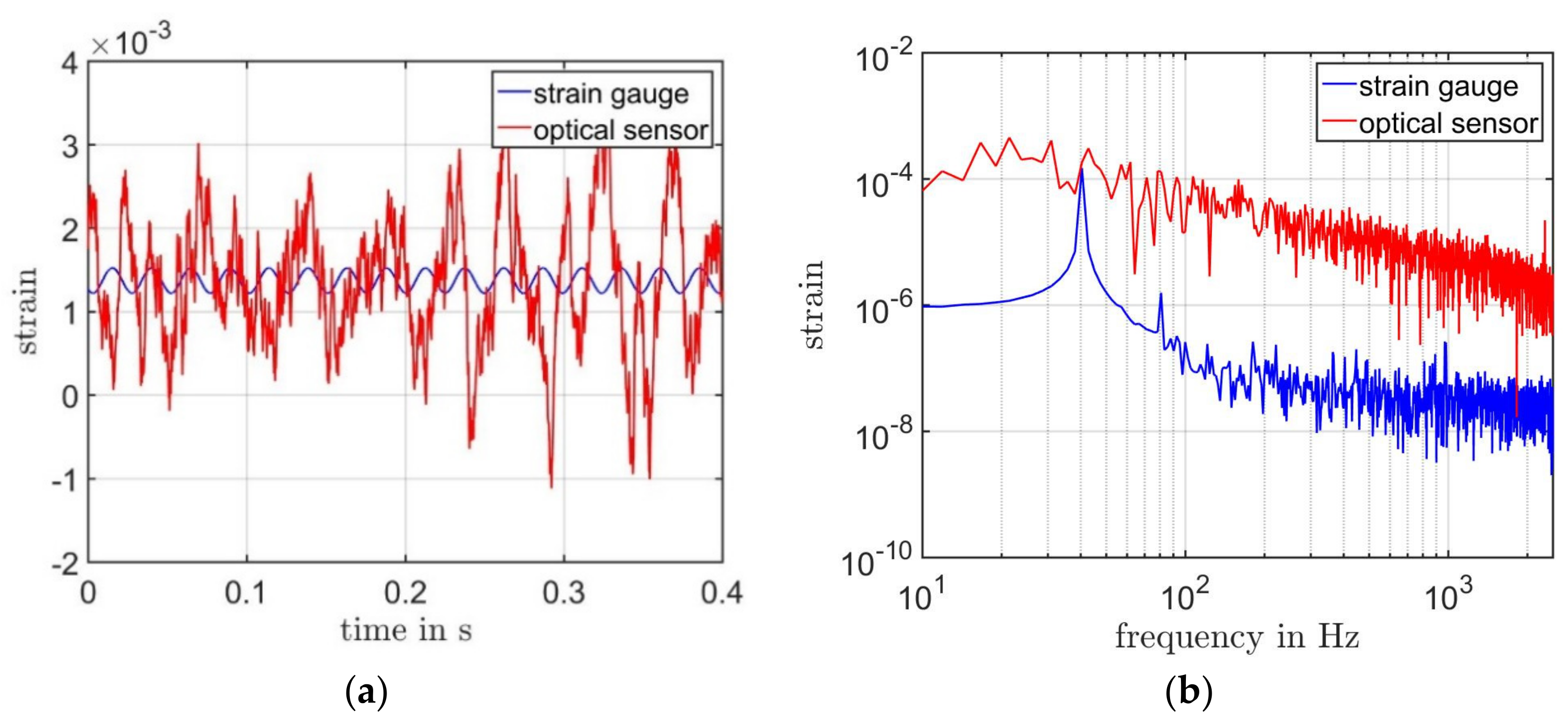
4. Experimental Setup and Results
5. Conclusions and Outlook
6. Patents
Author Contributions
Funding
Data Availability Statement
Conflicts of Interest
References
- Keil, S. Technology and Practical Use of Strain Gages with Particular Consideration of Stress Analysis Using Strain Gages; Ernst & Sohn: Berlin, Germany, 2017; pp. 17–108. [Google Scholar]
- Melle, S.; Alavie, A.; Karr, S.; Coroy, T.; Liu, K.; Measures, R. A Bragg grating-tuned fiber laser strain sensor system. IEEE Photon. Technol. Lett. 1993, 5, 263–266. [Google Scholar] [CrossRef]
- Barot, D.; Wang, G.; Duan, L. High-Resolution Dynamic Strain Sensor Using a Polarization-Maintaining Fiber Bragg Grating. IEEE Photon. Technol. Lett. 2019, 31, 709–712. [Google Scholar] [CrossRef]
- Pan, B.; Qian, K.; Xie, H.; Asundi, A. Two-dimensional digital image correlation for in-plane displacement and strain measurement: A review. Meas. Sci. Technol. 2009, 20, 20. [Google Scholar] [CrossRef]
- Khoo, S.-W.; Karuppanan, S.; Tan, C.-S. A Review of Surface Deformation and Strain Measurement Using Two-Dimensional Digital Image Correlation. Metrol. Meas. Syst. 2016, 23, 461–480. [Google Scholar] [CrossRef]
- Pan, B.; Tian, L. Advanced video extensometer for non-contact, real-time, high-accuracy strain measurement. Opt. Express 2016, 24, 19082–19093. [Google Scholar] [CrossRef]
- Tian, L.; Yu, L.; Pan, B. Accuracy enhancement of a video extensometer by real-time error compensation. Opt. Lasers Eng. 2018, 110, 272–278. [Google Scholar] [CrossRef]
- Pfeifer, T.; Mischo, H.K.; Ettemeyer, A.; Wang, Z.; Wegner, R. Strain/stress measurements using electronic speckle pattern interferometry. In Proceedings of the Three-Dimensional Imaging, Optical Metrology, and Inspection IV, Boston, MA, USA, 2–3 November 1998. [Google Scholar] [CrossRef]
- Zhu, Y.; Vaillant, J.; Montay, G.; François, M.; Hadjar, Y.; Bruyant, A. Simultaneous 2D in-plane deformation measurement using electronic speckle pattern interferometry with double phase modulations. Chin. Opt. Lett. 2018, 16, 071201. [Google Scholar]
- Yamaguchi, I.; Takemori, T.; Kobayashi, K. Stabilized and accelerated speckle strain gauge. Opt. Eng. 1993, 32, 618–625. [Google Scholar] [CrossRef]
- Pang, Y.; Chen, B.K.; Yu, S.F.; Lingamanaik, S.N. Enhanced laser speckle optical sensor for in situ strain sensing and structural health monitoring. Opt. Lett. 2020, 45, 2331–2334. [Google Scholar] [CrossRef]
- Wang, W.; Xu, C.; Jin, H.; Meng, S.; Zhang, Y.; Xie, W. Measurement of high temperature full-field strain up to 2000 °C using digital image correlation. Meas. Sci. Technol. 2017, 28, 035007. [Google Scholar] [CrossRef]
- Pan, Z.; Huang, S.; Su, Y.; Qiao, M.; Zhang, Q. Strain field measurements over 3000 °C using 3D-Digital image correlation. Opt. Lasers Eng. 2020, 127, 105942. [Google Scholar] [CrossRef]
- Hung, Y.; Ho, H.P. Shearography: An optical measurement technique and applications. Mater. Sci. Eng. R Rep. 2005, 49, 61–87. [Google Scholar] [CrossRef]
- Francis, D.; Tatam, R.P.; Groves, R.M. Shearography technology and applications: A review. Meas. Sci. Technol. 2010, 21, 21. [Google Scholar] [CrossRef]
- Xie, X.; Chen, X.; Li, J.; Wang, Y.; Yang, L. Measurement of in-plane strain with dual beam spatial phase-shift digital shearography. Meas. Sci. Technol. 2015, 26, 115202. [Google Scholar] [CrossRef]
- Cazzolato, B.; Wildy, S.; Codrington, J.; Kotousov, A.; Schuessler, M. Scanning Laser Vibrometer for Non-Contact Three-Dimensional Displacement and Strain Measurements. In Proceedings of the Australian Acoustical Society Conference, Geelong, Australia, 24–26 November 2008. [Google Scholar]
- Weisbecker, H.; Cazzolato, B.S.; Wildy, S.; Marburg, S.; Codrington, J.; Kotousov, A.; Kotousov, A. Surface Strain Measurements Using a 3D Scanning Laser Vibrometer. Exp. Mech. 2011, 52, 805–815. [Google Scholar] [CrossRef]
- Reyes, J.M.; Avitabile, P. Use of 3D Scanning Laser Vibrometer for Full Field Strain Measurements. In Experimental Techniques, Rotating Machinery, and Acoustics; The Society for Experimental Mechanics Series; Springer: Cham, Switzerland, 2015; Volume 8, pp. 197–209. [Google Scholar] [CrossRef]
- Jakobsen, M.L.; Hanson, S.G. Lenticular array for spatial filtering velocimetry of laser speckles from solid surfaces. Appl. Opt. 2004, 43, 4643–4651. [Google Scholar] [CrossRef]
- Jakobsen, M.L.; Larsen, H.E.; Hanson, S.G. Optical spatial filtering velocimetry sensor for sub-micron, in-plane vibration measurements. J. Opt. A Pure Appl. Opt. 2005, 7, S303–S307. [Google Scholar] [CrossRef]
- Aizu, Y.; Asakura, T. Spatial Filtering Velocimetry; Springer Science and Business Media LLC: Cham, Switzerland, 2005; pp. 139–170. [Google Scholar] [CrossRef]
- Albrecht, H.-E.; Borys, I.M.; Damaschke, D.-I.N.; Tropea, I.C. Basic Measurement Principles. In Laser Doppler and Phase Doppler Measurement Techniques; Springer Science and Business Media LLC: Cham, Switzerland, 2003; pp. 9–26. [Google Scholar] [CrossRef]
- Hercher, M.; Wyntjes, G.; Deweerd, H. Non-Contact Laser Extensometer. In Proceedings of the Industrial Laser Interferometry, Los Angeles, CA, USA, 10 September 1987; Volume 746, pp. 185–193. [Google Scholar] [CrossRef]
- Bin, L.; Jing-Wen, L.; Chun-Yong, Y. Study on the measurement of in-plane displacement of solid surfaces by laser Doppler velocimetry. Opt. Laser Technol. 1995, 27, 89–93. [Google Scholar] [CrossRef]
- Gasparetti, M.; Revel, G.M. The influence of operating conditions on the accuracy of in-plane laser Doppler velocimetry measurements. Measurement 1999, 26, 207–220. [Google Scholar] [CrossRef]
- Zhong, Y.; Zhang, G.; Leng, C.; Zhang, T. A differential laser Doppler system for one-dimensional in-plane motion measurement of MEMS. Measurement 2007, 40, 623–627. [Google Scholar] [CrossRef]
- Agusanto, K.; Lau, G.-K.; Wu, K.; Liu, T.; Zhu, C.; Yuan, L. Directional-sensitive differential laser Doppler vibrometry for in-plane motion measurement of specular surface. In Proceedings of the International Conference on Experimental Mechanics 2014, Singapore, 15–17 November 2014. [Google Scholar] [CrossRef]
- Wang, F.; Scholz, A.; Hug, J.; Rembe, C. Laser-Doppler-Dehnungssensor / Laser-Doppler strain gauge. TM Tech. Mess. 2019, 86, 82–86. [Google Scholar] [CrossRef]
- Rembe, C.; Siegmund, G.; Steger, H.; Wörtge, M. Measuring MEMS in Motion by Laser Doppler Vibrometry. In Optical Science and Engineering; Informa UK Limited: London, UK, 2006; pp. 245–292. [Google Scholar] [CrossRef]
- Dräbenstedt, A. Diversity combining in laser Doppler vibrometry for improved signal reliability. In Proceedings of the 11th International Conference on Vibration Measurements by Laser and Noncontact Techniques–Aivela 2014: Advances and Applications, Ancona, Italy, 25–27 June 2014. [Google Scholar] [CrossRef]
- Rembe, C.; Dräbenstedt, A. D1.1—Speckle-Insensitive Laser-Doppler Vibrometry with Adaptive Optics and Signal Diversity. In Proceedings SENSOR 2015; AMA Service GmbH: Wunstorf, Germany, 2015; pp. 505–510. [Google Scholar] [CrossRef]


| Parameter | Value | Parameter | Value | Parameter | Value |
|---|---|---|---|---|---|
Publisher’s Note: MDPI stays neutral with regard to jurisdictional claims in published maps and institutional affiliations. |
© 2021 by the authors. Licensee MDPI, Basel, Switzerland. This article is an open access article distributed under the terms and conditions of the Creative Commons Attribution (CC BY) license (http://creativecommons.org/licenses/by/4.0/).
Share and Cite
Wang, F.; Krause, S.; Hug, J.; Rembe, C. A Contactless Laser Doppler Strain Sensor for Fatigue Testing with Resonance-Testing Machine. Sensors 2021, 21, 319. https://doi.org/10.3390/s21010319
Wang F, Krause S, Hug J, Rembe C. A Contactless Laser Doppler Strain Sensor for Fatigue Testing with Resonance-Testing Machine. Sensors. 2021; 21(1):319. https://doi.org/10.3390/s21010319
Chicago/Turabian StyleWang, Fangjian, Steffen Krause, Joachim Hug, and Christian Rembe. 2021. "A Contactless Laser Doppler Strain Sensor for Fatigue Testing with Resonance-Testing Machine" Sensors 21, no. 1: 319. https://doi.org/10.3390/s21010319
APA StyleWang, F., Krause, S., Hug, J., & Rembe, C. (2021). A Contactless Laser Doppler Strain Sensor for Fatigue Testing with Resonance-Testing Machine. Sensors, 21(1), 319. https://doi.org/10.3390/s21010319