Expert Hypertension Detection System Featuring Pulse Plethysmograph Signals and Hybrid Feature Selection and Reduction Scheme

 , , ,
, , ,  and
and
Abstract
1. Introduction
Main Contributions
- This is the first study that used PuPG-based signals for the detection of hypertension.
- To accurately detect the hypertension pattern, we extract a large number of multi-domain features from preprocessed PuPG signals through discrete wavelet transform (DWT) and EMD.
- To reduce the feature dimensions and redundancy while improving the discriminative power of features, we proposed a hybrid feature selection and reduction (HFSR) scheme.
- The proposed expert hypertension detection system (EHDS) comprises preprocessing through EMD, followed by the feature extraction, kernel principal component analysis (KPCA), and weighted k-nearest neighbor (KNN-W) classifier, achieved an accuracy of 99.4%, sensitivity of 99.6%, and specificity of 99.4%.
2. Materials
2.1. Data Acquisition
2.2. Data Set Description
3. Methods
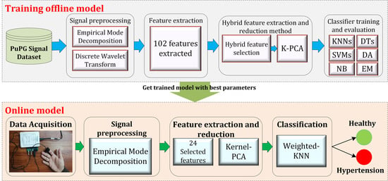
3.1. Design of the Study
- 1.
- Preprocessing: It removes the irrelevant information and artifacts from the acquired PuPG signal data of normal and hypertension classes. Method I employs discrete wavelet transform (DWT) for signal denoising through frequency and mean relative energy-based criteria. Method II adopts empirical mode decomposition (EMD) for noise elimination through analysis of mean frequencies and energies of individual signal components extracted from normal and hypertension classes.
- 2.
- Feature extraction: It extracts a combination of 102 features from preprocessed PuPG through DWT and EMD separately. These include time, frequency, spectral, texture, and cepstral features. The difference between signal classes is best captured through the extraction of a wide range of informative features.
- 3.
- Feature selection and reduction: This step eliminates features with redundant information through a hybrid feature selection and reduction (HFSR) method that is a combination of multiple feature ranking and transformation schemes. A high-dimensional feature vector is reduced through a new strategy of the averaging outcome of seven feature ranking methods, thus providing more reliable results. Next, we employed kernel principal component analysis (KPCA) to further decrease the feature dimension and represent significant information in fewer parameters. Extracted features in both method I and II are fed to the HFSR scheme to reduce the dimension of the resultant feature vector.
- 4.
- Classification:The final feature vectors extracted in both methods I and II of hypertension and normal classes are fed to a range of different classifiers, i.e, support vector machines (SVM), k-nearest neighbors (KNN), ensemble methods, decision trees (DT), and logistic regression (LR). Classification performance of both methods is evaluated through a baseline tenfold cross-validation strategy and compared with 5-, 15-, 20-, and 25-fold cross-validation.
3.2. Preprocessing
3.2.1. Discrete Wavelet Transform
3.2.2. Empirical Mode Decomposition
- In the entire signal, the total number of local extrema and zero crossings must be equal to each other or differ by a maximum one.
- The average of the envelopes computed through local minima and local maxima must be zero.
3.3. Feature Extraction
3.4. Hybrid Feature Selection and Reduction
3.4.1. Feature Selection Scheme
3.4.2. Feature Reduction Using Kernel PCA
3.5. Classification
4. Results
4.1. Method I
4.2. Method II
4.3. Method I versus Method II: A Comparative Analysis
5. Discussion
6. Conclusions
- The proposed EHDS system is based on the non-invasive methodology of PuPG signals.
- The EHDS is reliable and less computational intensive with high accuracy.
- The EHDS avoids overfitting as it is validated through 5-, 10-, 15-, and 20-fold cross-validation.
- The proposed approach does not only rely on morphological characteristics of the acquired signal.
- The method can be completely automated, and it works with all qualities of PuPG signals.
- The data set used in this research is yet small, with each sample with a length of 10 s.
- The procedure of initial feature extraction and selection of proper IMFs in EMD made the overall process strenuous and time-consuming.
Author Contributions
Funding
Institutional Review Board Statement
Informed Consent Statement
Data Availability Statement
Conflicts of Interest
References
- Tayefi, M.; Esmaeili, H.; Karimian, M.S.; Zadeh, A.A.; Ebrahimi, M.; Safarian, M.; Nematy, M.; Parizadeh, S.M.R.; Ferns, G.A.; Ghayour-Mobarhan, M. The application of a decision tree to establish the parameters associated with hypertension. Comput. Methods Programs Biomed. 2017, 139, 83–91. [Google Scholar] [CrossRef] [PubMed]
- WHO. Cardiovascular Diseases. 2017. Available online: https://www.who.int/news-room/fact-sheets/detail/cardiovascular-diseases-(cvds) (accessed on 23 October 2020).
- WHO. Hypertension, 13 September 2019. Available online: https://www.who.int/news-room/fact-sheets/detail/hypertension (accessed on 23 October 2020).
- Poddar, M.; Kumar, V.; Sharma, Y.P. Heart rate variability based classification of normal and hypertension cases by linear-nonlinear method. Def. Sci. J. 2014, 64, 542. [Google Scholar] [CrossRef]
- Li, W.; Gu, H.; Teo, K.K.; Bo, J.; Wang, Y.; Yang, J.; Wang, X.; Zhang, H.; Sun, Y.; Jia, X.; et al. Hypertension prevalence, awareness, treatment, and control in 115 rural and urban communities involving 47,000 people from China. J. Hypertens. 2016, 34, 39–46. [Google Scholar] [CrossRef] [PubMed]
- Wall, H.K.; Hannan, J.A.; Wright, J.S. Patients with undiagnosed hypertension: Hiding in plain sight. JAMA 2014, 312, 1973–1974. [Google Scholar] [CrossRef] [PubMed]
- Saleem, F.; Hassali, A.A.; Shafie, A.A. Hypertension in Pakistan: Time to take some serious action. Br. J. Gen. Pract. 2010, 60, 449–450. [Google Scholar] [CrossRef] [PubMed]
- Benjamin, E.J.; Blaha, M.J.; Chiuve, S.E.; Cushman, M.; Das, S.R.; Deo, R.; De Ferranti, S.D.; Floyd, J.; Fornage, M.; Gillespie, C.; et al. Heart disease and stroke statistics—2017 update. Circulation 2017, 135, e146–e603. [Google Scholar] [CrossRef]
- Goodhart, A.K. Hypertension from the patient’s perspective. Br. J. Gen. Pract. 2016, 66, 570. [Google Scholar] [CrossRef]
- Huang, C.; Wang, Y.; Li, X.; Ren, L.; Zhao, J.; Hu, Y.; Zhang, L.; Fan, G.; Xu, J.; Gu, X.; et al. Clinical features of patients infected with 2019 novel coronavirus in Wuhan, China. Lancet 2020, 395, 497–506. [Google Scholar] [CrossRef]
- Schiffrin, E.L.; Flack, J.M.; Ito, S.; Muntner, P.; Webb, R.C. Hypertension and COVID-19. Am. J. Hypertens. 2020, 33, 373–374. [Google Scholar] [CrossRef]
- Liang, Y.; Chen, Z.; Ward, R.; Elgendi, M.J.B. Photoplethysmography and deep learning: Enhancing hypertension risk stratification. Biosensors 2018, 8, 101. [Google Scholar] [CrossRef]
- Liang, Y.; Chen, Z.; Ward, R.; Elgendi, M. Hypertension assessment via ECG and PPG signals: An evaluation using MIMIC database. Diagnostics 2018, 8, 65. [Google Scholar] [CrossRef] [PubMed]
- Lan, K.C.; Raknim, P.; Kao, W.F.; Huang, J.H. Toward hypertension prediction based on PPG-derived HRV signals: A feasibility study. J. Med. Syst. 2018, 42, 103. [Google Scholar] [CrossRef] [PubMed]
- Ni, H.; Cho, S.; Mankoff, J.; Yang, J.J.; Computing, H. Automated recognition of hypertension through overnight continuous HRV monitoring. J. Ambient. Intell. Humaniz. Comput. 2018, 9, 2011–2023. [Google Scholar] [CrossRef]
- Kublanov, V.S.; Dolganov, A.Y.; Belo, D.; Gamboa, H.J. Comparison of machine learning methods for the arterial hypertension diagnostics. Appl. Bionics Biomech. 2017, 2017, 5985479. [Google Scholar] [CrossRef] [PubMed]
- Rajput, J.S.; Sharma, M.; Acharya, U.R. Hypertension Diagnosis Index for Discrimination of High-Risk Hypertension ECG Signals Using Optimal Orthogonal Wavelet Filter Bank. Int. J. Environ. Res. Public Health 2019, 16, 4068. [Google Scholar] [CrossRef]
- Soh, D.C.K.; Ng, E.; Jahmunah, V.; Oh, S.L.; San, T.R.; Acharya, U.R. A computational intelligence tool for the detection of hypertension using empirical mode decomposition. Medicine 2020, 118, 103630. [Google Scholar] [CrossRef]
- Liang, Y.; Chen, Z.; Ward, R.; Elgendi, M. Hypertension assessment using photoplethysmography: A risk stratification approach. J. Clin. Med. 2019, 8, 12. [Google Scholar] [CrossRef]
- Liu, F.; Zhou, X.; Wang, Z.; Cao, J.; Wang, H.; Zhang, Y. Unobtrusive mattress-based identification of hypertension by integrating classification and association rule mining. Sensors 2019, 19, 1489. [Google Scholar] [CrossRef]
- Baranchuk, A.; Kang, J.; Shaw, C.; Campbell, D.; Ribas, S.; Hopman, W.M.; Alanazi, H.; Redfearn, D.P.; Simpson, C.S. Electromagnetic interference of communication devices on ECG machines. Clin. Cardiol. Int. Index. Peer Rev. J. Adv. Treat. Cardiovasc. Dis. 2009, 32, 588–592. [Google Scholar] [CrossRef]
- Klein, A.; Djaiani, G. Mobile phones in the hospital–past, present and future. Anaesthesia 2003, 58, 353–357. [Google Scholar] [CrossRef]
- Kranjec, J.; Beguš, S.; Geršak, G.; Drnovšek, J. Non-contact heart rate and heart rate variability measurements: A review. Biomed. Signal Process. Control. 2014, 13, 102–112. [Google Scholar] [CrossRef]
- Ave, A.; Fauzan, H.; Adhitya, S.R.; Zakaria, H. Early detection of cardiovascular disease with photoplethysmogram (PPG) sensor. In Proceedings of the 2015 International Conference on Electrical Engineering and Informatics (ICEEI), Denpasar, Indonesia, 10–11 August 2015; pp. 676–681. [Google Scholar]
- Khan, M.U.; Aziz, S.; Malik, A.; Imtiaz, M.A. Detection of Myocardial Infarction using Pulse Plethysmograph Signals. In Proceedings of the 2019 International Conference on Frontiers of Information Technology (FIT), Islamabad, Pakistan, 16–18 December 2019; pp. 95–955. [Google Scholar]
- Khan, M.U.; Aziz, S.; Amjad, F.; Mohsin, M. Detection of Dilated Cardiomyopathy using Pulse Plethysmographic Signal Analysis. In Proceedings of the 2019 22nd International Multitopic Conference (INMIC), Islamabad, Pakistan, 29–30 November 2019; pp. 1–5. [Google Scholar]
- Khan, M.U.; Aziz, S.; Iqtidar, K.; Zainab, A.; Saud, A. Prediction of Acute Coronary Syndrome Using Pulse Plethysmograph. In Proceedings of the 2019 4th International Conference on Emerging Trends in Engineering, Sciences and Technology (ICEEST), Karachi, Pakistan, 10–11 December 2019; pp. 1–6. [Google Scholar]
- Naqvi, S.Z.H.; Aziz, S.; Khan, M.U.; Asghar, N.; Rasool, G. Emotion Recognition System using Pulse Plethysmograph. In Proceedings of the 2020 International Conference on Emerging Trends in Smart Technologies (ICETST), Karachi, Pakistan, 26–27 March 2020; pp. 1–6. [Google Scholar]
- Khan, M.U.; Aziz, S.; Naqvi, S.Z.H.; Zaib, A.; Maqsood, A. Pattern Analysis Towards Human Verification using Photoplethysmograph Signals. In Proceedings of the 2020 International Conference on Emerging Trends in Smart Technologies (ICETST), Karachi, Pakistan, 26–27 March 2020; pp. 1–6. [Google Scholar]
- Zhang, G.; Si, Y.; Yang, W.; Wang, D. A Robust Multilevel DWT Densely Network for Cardiovascular Disease Classification. Sensors 2020, 20, 4777. [Google Scholar] [CrossRef] [PubMed]
- Aileni, R.M.; Pasca, S.; Florescu, A. EEG-Brain Activity Monitoring and Predictive Analysis of Signals Using Artificial Neural Networks. Sensors 2020, 20, 3346. [Google Scholar] [CrossRef] [PubMed]
- Alturki, F.A.; AlSharabi, K.; Abdurraqeeb, A.M.; Aljalal, M. EEG Signal Analysis for Diagnosing Neurological Disorders Using Discrete Wavelet Transform and Intelligent Techniques. Sensors 2020, 20, 2505. [Google Scholar] [CrossRef] [PubMed]
- Gradolewski, D.; Redlarski, G. Wavelet-based denoising method for real phonocardiography signal recorded by mobile devices in noisy environment. Comput. Biol. Med. 2014, 52, 119–129. [Google Scholar] [CrossRef] [PubMed]
- Ebrahim, M.P.; Heydari, F.; Redoute, J.M.; Yuce, M.R. Accurate heart rate detection from on-body continuous wave radar sensors using wavelet transform. In Proceedings of the 2018 IEEE SENSORS, New Delhi, India, 28–31 October 2018; pp. 1–4. [Google Scholar]
- Ebrahim, M.P.; Heydari, F.; Walker, K.; Joe, K.; Redoute, J.M.; Yuce, M.R. Systolic Blood Pressure Estimation Using Wearable Radar and Photoplethysmogram Signals. In Proceedings of the 2019 IEEE International Conference on Systems, Man and Cybernetics (SMC), Bari, Italy, 6–9 October 2019; pp. 3878–3882. [Google Scholar]
- Asghar, M.A.; Khan, M.J.; Rizwan, M.; Mehmood, R.M.; Kim, S.H. An Innovative Multi-Model Neural Network Approach for Feature Selection in Emotion Recognition Using Deep Feature Clustering. Sensors 2020, 20, 3765. [Google Scholar] [CrossRef] [PubMed]
- Aziz, S.; Khan, M.U.; Alhaisoni, M.; Akram, T.; Altaf, M. Phonocardiogram Signal Processing for Automatic Diagnosis of Congenital Heart Disorders through Fusion of Temporal and Cepstral Features. Sensors 2020, 20, 3790. [Google Scholar] [CrossRef]
- Tsimpiris, A.; Kugiumtzis, D. Feature selection for classification of oscillating time series. Expert Syst. 2012, 29, 456–477. [Google Scholar] [CrossRef]
- Goyal, D.; Choudhary, A.; Pabla, B.; Dhami, S. Support vector machines based non-contact fault diagnosis system for bearings. J. Intell. Manuf. 2019, 31, 1275–1289. [Google Scholar] [CrossRef]
- Fasil, O.; Rajesh, R. Time-domain exponential energy for epileptic EEG signal classification. Neurosci. Lett. 2019, 694, 1–8. [Google Scholar]
- Banker, R.; Natarajan, R.; Zhang, D. Two-stage estimation of the impact of contextual variables in stochastic frontier production function models using data envelopment analysis: Second stage OLS versus bootstrap approaches. Eur. J. Oper. Res. 2019, 278, 368–384. [Google Scholar] [CrossRef]
- Kumar, D.; Carvalho, P.; Antunes, M.; Paiva, R.; Henriques, J. Heart murmur classification with feature selection. In Proceedings of the 2010 Annual International Conference of the IEEE Engineering in Medicine and Biology, Buenos Aires, Argentina, 31 August–4 September 2010; pp. 4566–4569. [Google Scholar]
- Dhindsa, I.S.; Agarwal, R.; Ryait, H.S. Performance evaluation of various classifiers for predicting knee angle from electromyography signals. Expert Syst. 2019, 36, e12381. [Google Scholar] [CrossRef]
- Mukhopadhyay, A.K.; Samui, S. An experimental study on upper limb position invariant EMG signal classification based on deep neural network. Biomed. Signal Process. Control. 2020, 55, 101669. [Google Scholar] [CrossRef]
- Phinyomark, A.; Phukpattaranont, P.; Limsakul, C. Feature reduction and selection for EMG signal classification. Expert Syst. Appl. 2012, 39, 7420–7431. [Google Scholar] [CrossRef]
- Peeters, G. A large set of audio features for sound description (similarity and classification) in the CUIDADO project. Cuid. IST Proj. Rep. 2004, 54, 1–25. [Google Scholar]
- Yadav, A.; Singh, A.; Dutta, M.K.; Travieso, C.M. Machine learning-based classification of cardiac diseases from PCG recorded heart sounds. Neural Comput. Appl. 2019, 1–14. [Google Scholar] [CrossRef]
- Amezquita-Sanchez, J.P.; Mammone, N.; Morabito, F.C.; Marino, S.; Adeli, H. A novel methodology for automated differential diagnosis of mild cognitive impairment and the Alzheimer’s disease using EEG signals. J. Neurosci. Methods 2019, 322, 88–95. [Google Scholar] [CrossRef]
- Peng, J.; Hao, D.; Yang, L.; Du, M.; Song, X.; Jiang, H.; Zhang, Y.; Zheng, D. Evaluation of electrohysterogram measured from different gestational weeks for recognizing preterm delivery: A preliminary study using random Forest. Biocybern. Biomed. Eng. 2020, 40, 352–362. [Google Scholar] [CrossRef]
- Birajdar, G.K.; Patil, M.D. Speech/music classification using visual and spectral chromagram features. J. Ambient. Intell. Humaniz. Comput. 2020, 11, 329–347. [Google Scholar] [CrossRef]
- Leite, J.P.R.; Moreno, R.L. Heartbeat classification with low computational cost using Hjorth parameters. IET Signal Process. 2017, 12, 431–438. [Google Scholar] [CrossRef]
- Dua, M.; Aggarwal, R.K.; Biswas, M. GFCC based discriminatively trained noise robust continuous ASR system for Hindi language. J. Ambient. Intell. Humaniz. Comput. 2019, 10, 2301–2314. [Google Scholar] [CrossRef]
- Adnan, S.M.; Irtaza, A.; Aziz, S.; Ullah, M.O.; Javed, A.; Mahmood, M.T. Fall detection through acoustic local ternary patterns. Appl. Acoust. 2018, 140, 296–300. [Google Scholar] [CrossRef]
- Guyon, I. Practical feature selection: From correlation to causality. In Proceedings of the NATO Advanced Study Institute on Mining Massive Data Sets for Security (MMDSS 2007), Gazzada, Italy, 10–21 September 2007; pp. 27–43. [Google Scholar]
- Li, X.; Ling, S.H.; Su, S. A Hybrid Feature Selection and Extraction Methods for Sleep Apnea Detection Using Bio-Signals. Sensors 2020, 20, 4323. [Google Scholar] [CrossRef]
- Zhen, Z.; Zeng, X.; Wang, H.; Han, L. A global evaluation criterion for feature selection in text categorization using Kullback-Leibler divergence. In Proceedings of the 2011 International Conference of Soft Computing and Pattern Recognition (SoCPaR), Dalian, China, 14–16 October 2011; pp. 440–445. [Google Scholar]
- Guorong, X.; Peiqi, C.; Minhui, W. Bhattacharyya distance feature selection. In Proceedings of the 13th International Conference on Pattern Recognition, Vienna, Austria, 25–29 August 1996; Volume 2, pp. 195–199. [Google Scholar]
- Chowdhury, M.H.; Shuzan, M.N.I.; Chowdhury, M.E.; Mahbub, Z.B.; Uddin, M.M.; Khandakar, A.; Reaz, M.B.I. Estimating Blood Pressure from the Photoplethysmogram Signal and Demographic Features Using Machine Learning Techniques. Sensors 2020, 20, 3127. [Google Scholar] [CrossRef] [PubMed]
- Ding, C.; Peng, H. Minimum redundancy feature selection from microarray gene expression data. J. Bioinform. Comput. Biol. 2005, 3, 185–205. [Google Scholar] [CrossRef] [PubMed]
- Xu, Y.; Zhao, X.; Chen, Y.; Zhao, W. Research on a mixed gas recognition and concentration detection algorithm based on a metal oxide semiconductor olfactory system sensor array. Sensors 2018, 18, 3264. [Google Scholar] [CrossRef] [PubMed]
- Schölkopf, B.; Smola, A.; Müller, K.R. Nonlinear component analysis as a kernel eigenvalue problem. Neural Comput. 1998, 10, 1299–1319. [Google Scholar] [CrossRef]
- Khan, M.U.; Saad, M.; Aziz, S.; Ch, J.M.; Naqvi, S.Z.H.; Qasim, M.A. Electrocardiogram based Gender Classification. In Proceedings of the 2020 International Conference on Electrical, Communication, and Computer Engineering (ICECCE), Istanbul, Turkey, 12–13 June 2020; pp. 1–6. [Google Scholar]
- Hoffmann, H. Kernel PCA for novelty detection. Pattern Recognit. 2007, 40, 863–874. [Google Scholar] [CrossRef]
- Mohamed, M.; Deriche, M. An approach for ECG feature extraction using daubechies 4 (DB4) wavelet. Int. J. Comput. Appl. 2014, 96, 36–41. [Google Scholar]
- Acharya, U.R.; Fujita, H.; Adam, M.; Lih, O.S.; Sudarshan, V.K.; Hong, T.J.; Koh, J.E.; Hagiwara, Y.; Chua, C.K.; Poo, C.K.; et al. Automated characterization and classification of coronary artery disease and myocardial infarction by decomposition of ECG signals: A comparative study. Inf. Sci. 2017, 377, 17–29. [Google Scholar] [CrossRef]
- Labate, D.; La Foresta, F.; Occhiuto, G.; Morabito, F.C.; Lay-Ekuakille, A.; Vergallo, P. Empirical mode decomposition vs. wavelet decomposition for the extraction of respiratory signal from single-channel ECG: A comparison. IEEE Sens. J. 2013, 13, 2666–2674. [Google Scholar] [CrossRef]
- Mills, K.T.; Bundy, J.D.; Kelly, T.N.; Reed, J.E.; Kearney, P.M.; Reynolds, K.; Chen, J.; He, J. Global disparities of hypertension prevalence and control: A systematic analysis of population-based studies from 90 countries. Circulation 2016, 134, 441–450. [Google Scholar] [CrossRef] [PubMed]


| Class | Systolic (mmHg) | Diastolic (mmHg) |
|---|---|---|
| Optimal | Less than 120 | Less than 80 |
| Normal | 120 to 129 | 80 to 84 |
| High Normal | 130 to 139 | 85 to 89 |
| Hypertension | More than or equal to 140 | More than or equal to 90 |
| Type | Photoplethysmograph (PPG) Sensor | Pulse Plethysmograph (PuPG) Sensor |
|---|---|---|
| Input signal | Optical signal | Pressure changes |
| Phenomenon | Blood volumetric changes are detected by measuring the amount of light transmitted or reflected by the sensor. | Blood volumetric changes are detected by the piezoelectric material of the sensor as pressure changes when the blood volume changes. |
| Noise Impact | Light signal can be easily impacted by any external light changes. Dirty hand can distort the light intensities. | Piezoelectric material based sensors are normaly temperature sensitive. Dirty hands or foreign material on hand or fingers does not have significant impact. |
| Data Class | Subjects | Age Group | Samples |
|---|---|---|---|
| Hypertension | Male: 29 | Male: 40–76 | 700 |
| Female: 27 | Female: 39–59 | ||
| Normal | Male: 35 | Male: 21–63 | 709 |
| Female: 30 | Female: 20–59 | ||
| Overall | 121 | 20–76 | 1409 |
| Decomposition Levels | Frequency Range (Hz) | Mean Relative Energy (%) | |
|---|---|---|---|
| Normal | Hypertension | ||
| 250–500 | 0.07% | 0.59% | |
| 122–256 | 0.09% | 0.32% | |
| 61.1–128 | 0.19% | 0.35% | |
| 30.6–63.9 | 0.46% | 0.49% | |
| 15.3–31.9 | 1.93% | 3.10% | |
| 7.65–16 | 14.77% | 13.31% | |
| 3.84–7.97 | 31.03% | 21.49% | |
| 1.94–3.99 | 29.11% | 19.05% | |
| 1.03–1.99 | 21.11% | 26.77% | |
| 0.594–0.958 | 0.16% | 7.65% | |
| 0–0.431 | 1.08% | 6.88% | |
| 0–31.2 | 99.19% | 98.26% | |
| Components | Normal | Hypertension | ||
|---|---|---|---|---|
| Mean Frequency Range (Hz) | Mean Relative Energy (%) | Mean Frequency Range (Hz) | Mean Relative Energy (%) | |
| 103–483 | 0.00 | 86.5–484 | 1.02 | |
| 11.3–60.2 | 0.14 | 40.7–219 | 0.35 | |
| 3.09–14 | 30.34 | 3.3–61 | 2.04 | |
| 2.99–12.2 | 4.97 | 3.34–23.3 | 6.65 | |
| 1.28–10 | 22.76 | 2.98–11.4 | 14.95 | |
| Residual | 0.129–5.55 | 41.78 | 0.0197–4.33 | 74.99 |
| Method I | Method II | |||||||
|---|---|---|---|---|---|---|---|---|
| Feature | Normal | Hypertension | Normal | Hypertension | ||||
| Mean | STD | Mean | STD | Mean | STD | Mean | STD | |
| Mean | 0.008 | 0.027 | 0.017 | 0.031 | 0.001 | 0.049 | 0.013 | 0.053 |
| Standard Deviation | 0.253 | 0.032 | 0.250 | 0.046 | 0.254 | 0.032 | 0.248 | 0.045 |
| Skewness | −1.959 | 0.522 | −2.144 | 0.651 | −1.997 | 0.576 | −2.220 | 0.641 |
| Kurtosis | 6.993 | 1.499 | 8.083 | 3.864 | 7.139 | 1.688 | 8.297 | 3.944 |
| Peak to Peak Value | 1.380 | 0.199 | 1.398 | 0.140 | 1.377 | 0.178 | 1.375 | 0.144 |
| Root Mean Square | 0.255 | 0.033 | 0.252 | 0.047 | 0.258 | 0.038 | 0.254 | 0.046 |
| Crest Factor | 1.659 | 0.939 | 1.635 | 0.381 | 1.587 | 0.991 | 1.523 | 0.536 |
| Shape Factor | 1.484 | 0.134 | 1.458 | 0.159 | 1.522 | 0.163 | 1.465 | 0.167 |
| Impulse Factor | 2.435 | 1.297 | 2.382 | 0.593 | 2.371 | 1.376 | 2.171 | 0.632 |
| Margin Factor | 15.22 | 14.64 | 15.12 | 7.27 | 15.16 | 15.56 | 13.39 | 6.45 |
| Energy | 389.6 | 209.7 | 437.4 | 207.6 | 393.9 | 207.4 | 448.5 | 222.5 |
| Peak to RMS Value | 3.894 | 0.623 | 4.094 | 0.991 | 3.921 | 0.663 | 4.108 | 1.102 |
| Root Sum of Squares | 18.933 | 5.600 | 20.292 | 5.089 | 19.069 | 5.525 | 20.480 | 5.412 |
| Shannon Energy | 549.7 | 312.3 | 618.2 | 279.7 | 526.6 | 295.8 | 686.5 | 414.4 |
| Log Energy | −27,888 | 15,515 | −34,569 | 18,644 | −28,509 | 16,289 | −32,613 | 16,387 |
| Mean Absolute Deviation | 0.169 | 0.026 | 0.169 | 0.043 | 0.169 | 0.028 | 0.168 | 0.043 |
| Median Absolute Deviation | 0.074 | 0.026 | 0.071 | 0.030 | 0.071 | 0.033 | 0.059 | 0.024 |
| Average Frequency | 0.002 | 0.001 | 0.001 | 0.001 | 0.002 | 0.003 | 0.002 | 0.002 |
| Jitter | 137.1 | 180.9 | 85.5 | 150.4 | 159.0 | 248.8 | 52.0 | 95.8 |
| Spectral Mean | 3.144 | 5.928 | 0.771 | 1.960 | 8.623 | 15.700 | 2.764 | 6.372 |
| Spectral Standard Deviation | 3.401 | 4.833 | 1.549 | 3.463 | 7.571 | 11.498 | 3.031 | 6.016 |
| Spectral Skewness | 2.361 | 1.496 | 3.763 | 1.295 | 0.996 | 1.360 | 1.797 | 1.908 |
| Specral Kurtosis | 11.331 | 8.235 | 20.190 | 9.589 | 5.588 | 4.947 | 10.564 | 8.751 |
| Spectral Centroid | 9.442 | 0.202 | 9.915 | 1.481 | 9.771 | 1.576 | 10.768 | 2.216 |
| Spectral Flux | 0.008 | 0.002 | 0.008 | 0.002 | 0.008 | 0.002 | 0.008 | 0.002 |
| Spectral Roll-off | 91.699 | 1.010 | 96.587 | 8.383 | 97.036 | 10.371 | 136.257 | 44.372 |
| Spectral Flatness | 0.025 | 0.014 | 0.051 | 0.035 | 0.063 | 0.065 | 0.171 | 0.138 |
| Spectral Crest | 0.642 | 0.012 | 0.621 | 0.040 | 0.631 | 0.030 | 0.593 | 0.059 |
| Spectral Decrease | −4.333 | 0.228 | −4.013 | 0.658 | −4.169 | 0.538 | −3.656 | 0.830 |
| Spectral Slope | −0.023 | 0.003 | −0.023 | 0.003 | −0.024 | 0.003 | −0.023 | 0.005 |
| Spectral Spread | 18.505 | 0.199 | 19.029 | 1.178 | 19.328 | 1.617 | 23.521 | 5.818 |
| Mean Frequency | 4.347 | 0.949 | 4.999 | 3.451 | 4.989 | 3.063 | 6.446 | 4.440 |
| Median Frequency | 3.574 | 0.803 | 2.972 | 0.880 | 3.811 | 3.573 | 2.846 | 0.753 |
| Spurious-free Dynamic Range | 3.073 | 6.019 | 2.196 | 2.107 | 3.163 | 6.451 | 2.056 | 1.812 |
| Signal to Noise Distortion | −0.885 | 6.041 | −2.036 | 3.101 | −0.755 | 6.819 | −2.097 | 3.030 |
| Total Harmonic Distortions | −2.376 | 5.452 | −0.938 | 4.964 | −3.144 | 6.562 | −0.396 | 4.110 |
| 1st Coeffient of MFCC | −44.99 | 0.37 | −44.716 | 0.512 | −44.84 | 0.60 | −44.45 | 0.80 |
| 2nd Coeffient of MFCC | 6.268 | 0.523 | 6.661 | 0.714 | 6.480 | 0.846 | 7.028 | 1.122 |
| 3rd Coeffient of MFCC | 5.976 | 0.499 | 6.350 | 0.683 | 6.169 | 0.802 | 6.690 | 1.066 |
| 4th Coeffient of MFCC | 5.508 | 0.462 | 5.851 | 0.634 | 5.671 | 0.733 | 6.148 | 0.976 |
| 1st Coeffient of GFCC | −7.183 | 0.430 | −6.762 | 0.610 | −7.027 | 0.793 | −6.220 | 1.266 |
| 2nd Coeffient of GFCC | 1.844 | 0.063 | 1.869 | 0.071 | 1.522 | 0.419 | 1.119 | 0.574 |
| 3rd Coeffient of GFCC | 0.553 | 0.138 | 0.367 | 0.269 | 0.643 | 0.105 | 0.492 | 0.206 |
| 4th Coeffient of GFCC | 0.301 | 0.024 | 0.266 | 0.033 | 0.392 | 0.109 | 0.408 | 0.109 |
| 1st Coefficient of Chroma Vector | 0.383 | 0.235 | 0.750 | 0.501 | 0.653 | 0.532 | 2.126 | 1.930 |
| 2nd Coefficient of Chroma Vector | 0.416 | 0.258 | 0.773 | 0.518 | 0.663 | 0.546 | 2.130 | 1.948 |
| 3rd Coefficient of Chroma Vector | 0.433 | 0.269 | 0.842 | 0.575 | 0.742 | 0.672 | 2.129 | 2.144 |
| 4th Coefficient of Chroma Vector | 0.623 | 0.378 | 1.297 | 0.942 | 0.700 | 0.568 | 2.011 | 2.046 |
| 5th Coefficient of Chroma Vector | 0.564 | 0.337 | 1.212 | 0.872 | 0.691 | 0.534 | 2.044 | 1.935 |
| 6th Coefficient of Chroma Vector | 0.527 | 0.320 | 1.230 | 0.987 | 0.748 | 0.563 | 2.227 | 2.267 |
| 7th Coefficient of Chroma Vector | 0.483 | 0.296 | 1.069 | 0.760 | 0.705 | 0.524 | 2.107 | 1.893 |
| 8th Coefficient of Chroma Vector | 0.451 | 0.279 | 0.982 | 0.696 | 0.686 | 0.528 | 2.071 | 1.863 |
| 9th Coefficient of Chroma Vector | 0.429 | 0.268 | 0.908 | 0.638 | 0.679 | 0.529 | 2.099 | 1.929 |
| 10th Coefficient of Chroma Vector | 0.400 | 0.251 | 0.878 | 0.609 | 0.651 | 0.537 | 2.087 | 1.848 |
| 11th Coefficient of Chroma Vector | 0.373 | 0.232 | 0.776 | 0.537 | 0.668 | 0.522 | 2.106 | 1.954 |
| 12th Coefficient of Chroma Vector | 0.348 | 0.225 | 0.705 | 0.474 | 0.622 | 0.522 | 2.078 | 1.890 |
| Enhanced Mean Absolute Value | 0.297 | 0.039 | 0.302 | 0.055 | 0.294 | 0.052 | 0.301 | 0.049 |
| Enhanced Wavelength | 236.4 | 133.5 | 413.7 | 319.8 | 284.3 | 198.6 | 665.7 | 515.0 |
| Wavelength | 36.83 | 21.94 | 85.59 | 96.94 | 54.42 | 46.94 | 193.47 | 186.80 |
| Slope Sign Change | 45.1 | 86.9 | 508.4 | 549.0 | 1039.5 | 1657.6 | 3463.1 | 2792.1 |
| Average Amplitude Change | 0.006 | 0.003 | 0.010 | 0.009 | 0.009 | 0.009 | 0.021 | 0.018 |
| Difference Absolute Std. Dev. | 0.009 | 0.003 | 0.013 | 0.010 | 0.014 | 0.010 | 0.027 | 0.021 |
| Log Detector | 0.108 | 0.030 | 0.118 | 0.037 | 0.107 | 0.043 | 0.117 | 0.036 |
| Modified Mean Absolute Value | 0.130 | 0.025 | 0.133 | 0.034 | 0.130 | 0.033 | 0.132 | 0.030 |
| Modified Mean Absolute Value 2 | 0.083 | 0.022 | 0.089 | 0.026 | 0.084 | 0.027 | 0.087 | 0.020 |
| Pulse Percentage Rate | 0.939 | 0.029 | 0.953 | 0.027 | 0.937 | 0.045 | 0.957 | 0.035 |
| Simple Square Integral | 389.6 | 209.7 | 437.4 | 207.6 | 393.9 | 207.4 | 448.5 | 222.5 |
| Willison Amplitude | 1153.6 | 765.6 | 2670.8 | 2603.9 | 1836.0 | 1707.6 | 4551.3 | 3502.4 |
| Maximum Fractal Length | −0.463 | 0.384 | −0.136 | 0.740 | −0.174 | 0.594 | 0.428 | 1.121 |
| Root Squared Zero Order Moment | 2.592 | 0.032 | 2.600 | 0.026 | 2.593 | 0.031 | 2.601 | 0.028 |
| Root Squared 2nd Order Moment | 2.068 | 0.066 | 2.036 | 0.062 | 1.984 | 0.115 | 1.913 | 0.130 |
| Root Squared 4th Order Moment | 2.045 | 0.077 | 2.001 | 0.078 | 1.891 | 0.159 | 1.794 | 0.205 |
| Sparseness | 0.535 | 0.064 | 0.582 | 0.086 | 0.655 | 0.137 | 0.747 | 0.188 |
| Irregularity Factor | −0.464 | 0.037 | −0.445 | 0.047 | −0.446 | 0.058 | −0.406 | 0.061 |
| Waveform Length Ratio | −0.065 | 0.703 | −0.354 | 0.230 | −0.648 | 0.604 | −0.721 | 0.727 |
| Complexity | 0.502 | 0.222 | 0.706 | 0.253 | 0.897 | 0.524 | 1.314 | 0.515 |
| Mobility | 0.038 | 0.011 | 0.057 | 0.038 | 0.055 | 0.035 | 0.115 | 0.079 |
| Higuchi’s Fractal Dimension | 1.054 | 0.052 | 1.149 | 0.119 | 1.183 | 0.240 | 1.490 | 0.401 |
| Katz Fractal Dimension | 1.000 | 0.000 | 1.000 | 0.000 | 1.000 | 0.000 | 1.000 | 0.000 |
| Lyapunov Exponent | 437.4 | 49.5 | 394.8 | 49.3 | 362.9 | 78.8 | 239.1 | 92.2 |
| Approximate Entropy | 0.104 | 0.049 | 0.155 | 0.134 | 0.127 | 0.080 | 0.316 | 0.312 |
| Correlation Dimension | 1.687 | 0.168 | 1.733 | 0.191 | 1.676 | 0.202 | 1.731 | 0.300 |
| 1st Coefficient of LTP | 259.6 | 128.8 | 291.5 | 122.1 | 259.6 | 128.8 | 291.5 | 122.1 |
| 2nd Coefficient of LTP | 40.790 | 30.943 | 56.809 | 35.998 | 40.790 | 30.943 | 56.809 | 35.998 |
| 3rd Coefficient of LTP | 24.574 | 23.717 | 41.723 | 32.083 | 24.574 | 23.717 | 41.723 | 32.083 |
| 4th Coefficient of LTP | 16.381 | 15.761 | 30.738 | 22.667 | 16.381 | 15.761 | 30.738 | 22.667 |
| 5th Coefficient of LTP | 18.472 | 15.755 | 33.411 | 24.881 | 18.472 | 15.755 | 33.411 | 24.881 |
| 6th Coefficient of LTP | 25.205 | 21.607 | 45.518 | 33.715 | 25.205 | 21.607 | 45.518 | 33.715 |
| 7th Coefficient of LTP | 17.699 | 16.352 | 29.035 | 22.609 | 17.699 | 16.352 | 29.035 | 22.609 |
| 8th Coefficient of LTP | 26.261 | 23.075 | 39.645 | 28.386 | 26.261 | 23.075 | 39.645 | 28.386 |
| 9th Coefficient of LTP | 47.483 | 32.844 | 58.163 | 35.132 | 47.483 | 32.844 | 58.163 | 35.132 |
| 10th Coefficient of LTP | 207.278 | 94.769 | 201.809 | 72.537 | 207.278 | 94.769 | 201.809 | 72.537 |
| 11th Coefficient of LTP | 269.5 | 137.7 | 302.1 | 121.7 | 269.5 | 137.70 | 302.1 | 121.7 |
| 12th Coefficient of LTP | 41.733 | 31.354 | 59.773 | 38.092 | 41.733 | 31.354 | 59.773 | 38.092 |
| 13th Coefficient of LTP | 24.006 | 23.096 | 41.071 | 31.294 | 24.006 | 23.096 | 41.071 | 31.294 |
| 14th Coefficient of LTP | 16.784 | 15.900 | 30.199 | 23.471 | 16.784 | 15.900 | 30.199 | 23.471 |
| 15th Coefficient of LTP | 18.506 | 15.140 | 33.390 | 25.583 | 18.506 | 15.140 | 33.390 | 25.583 |
| 16th Coefficient of LTP | 26.148 | 22.755 | 44.177 | 31.682 | 26.148 | 22.755 | 44.177 | 31.682 |
| 17th Coefficient of LTP | 16.898 | 16.559 | 30.149 | 21.910 | 16.898 | 16.559 | 30.149 | 21.910 |
| 18th Coefficient of LTP | 25.790 | 22.892 | 39.312 | 26.784 | 25.790 | 22.892 | 39.312 | 26.784 |
| 19th Coefficient of LTP | 46.534 | 33.045 | 56.298 | 33.647 | 46.534 | 33.045 | 56.298 | 33.647 |
| 20th Coefficient of LTP | 197.773 | 85.090 | 191.858 | 74.487 | 197.773 | 85.090 | 191.858 | 74.487 |
| Feature | TT | KLD | BD | ROC | MWT | MRMR | RRF | MR |
|---|---|---|---|---|---|---|---|---|
| 3rd Coefficient of LTP | 12 | 93 | 93 | 83 | 32 | 102 | 98 | 73.29 |
| 6th Coefficient of Chroma Vector | 38 | 98 | 76 | 79 | 78 | 94 | 49 | 73.14 |
| Lyapunov Exponent | 93 | 92 | 92 | 70 | 81 | 10 | 70 | 72.57 |
| Sparseness | 70 | 90 | 90 | 30 | 62 | 79 | 84 | 72.14 |
| Jitter | 78 | 58 | 58 | 74 | 77 | 85 | 74 | 72.00 |
| 9th Coefficient of LTP | 57 | 83 | 83 | 75 | 82 | 92 | 24 | 70.86 |
| Spectral Decrease | 62 | 28 | 61 | 85 | 75 | 93 | 83 | 69.57 |
| 4th Coefficient of MFCC | 96 | 41 | 41 | 95 | 40 | 72 | 99 | 69.14 |
| Irregularity | 35 | 94 | 100 | 57 | 88 | 90 | 13 | 68.14 |
| 1st Coeffient of MFCC | 99 | 23 | 23 | 100 | 37 | 96 | 97 | 67.86 |
| Waveform Length Ratio | 13 | 100 | 94 | 91 | 9 | 100 | 66 | 67.57 |
| 3rd Coeffient of MFCC | 79 | 97 | 97 | 84 | 39 | 55 | 17 | 66.86 |
| 1st Coefficient of Chroma Vector | 71 | 86 | 86 | 98 | 26 | 48 | 53 | 66.86 |
| Spectral Roll-off | 81 | 43 | 79 | 66 | 56 | 59 | 81 | 66.43 |
| Spectral Crest | 61 | 80 | 60 | 26 | 92 | 71 | 75 | 66.43 |
| 6th Coefficient of Chroma Vector | 100 | 76 | 99 | 31 | 61 | 45 | 52 | 66.29 |
| 7th Coefficient of Chroma Vector | 37 | 99 | 98 | 1 | 96 | 42 | 86 | 65.57 |
| Median Frequency | 88 | 35 | 78 | 71 | 102 | 78 | 2 | 64.86 |
| 2nd Coefficient of Chroma Vector | 89 | 7 | 96 | 89 | 41 | 81 | 51 | 64.86 |
| Spectral Centroid | 76 | 79 | 43 | 39 | 86 | 69 | 58 | 64.29 |
| Difference Absolute Std. Dev. Value | 84 | 38 | 37 | 81 | 79 | 63 | 64 | 63.71 |
| Shape Factor | 59 | 53 | 53 | 54 | 72 | 80 | 73 | 63.43 |
| Spectral Mean | 43 | 77 | 77 | 96 | 46 | 40 | 61 | 62.86 |
| Simple Square Integral | 4 | 72 | 72 | 22 | 89 | 89 | 92 | 62.86 |
| 3rd Coefficient of GFCC | 95 | 29 | 88 | 94 | 34 | 53 | 45 | 62.57 |
| 4th Coefficient of Chroma Vector | 40 | 96 | 30 | 87 | 85 | 52 | 47 | 62.43 |
| Root Mean Square | 45 | 56 | 56 | 77 | 43 | 87 | 69 | 61.86 |
| Signal to Noise Distortion | 97 | 69 | 69 | 47 | 74 | 31 | 42 | 61.29 |
| 9th Coefficient of Chroma Vector | 72 | 12 | 95 | 88 | 27 | 76 | 57 | 61.00 |
| Mean Absolute Deviation | 58 | 48 | 48 | 49 | 76 | 82 | 62 | 60.43 |
| Root Squared 2nd Order Moment | 91 | 82 | 71 | 8 | 59 | 20 | 91 | 60.29 |
| Root Squared 4th Order Moment | 101 | 71 | 82 | 82 | 4 | 66 | 14 | 60.00 |
| 10th Coefficient of Chroma Vector | 36 | 95 | 85 | 28 | 73 | 41 | 56 | 59.14 |
| 12th Coefficient of Chroma Vector | 90 | 89 | 89 | 59 | 10 | 37 | 38 | 58.86 |
| 1st Coefficient of GFCC | 69 | 87 | 87 | 61 | 66 | 38 | 3 | 58.71 |
| Mean | 80 | 26 | 26 | 80 | 80 | 68 | 44 | 57.71 |
| Enhanced Mean Absolute Value | 21 | 73 | 73 | 62 | 58 | 54 | 63 | 57.71 |
| Root Sum of Squares | 53 | 49 | 52 | 99 | 18 | 58 | 72 | 57.29 |
| 2nd Coefficient of LTP | 82 | 70 | 70 | 35 | 36 | 12 | 95 | 57.14 |
| Katz Fractal Dimension | 67 | 3 | 3 | 67 | 90 | 75 | 90 | 56.43 |
| Feature | TT | KLD | BD | ROC | MWT | MRMR | RRF | MR |
|---|---|---|---|---|---|---|---|---|
| 7th Coefficient of Chroma Vector | 100 | 98 | 98 | 26 | 96 | 97 | 55 | 81.43 |
| 4th Coefficient of Chroma Vector | 89 | 96 | 76 | 73 | 85 | 52 | 96 | 81.00 |
| Mobility | 93 | 64 | 64 | 67 | 68 | 91 | 95 | 77.43 |
| Spectral Centroid | 68 | 78 | 78 | 77 | 45 | 98 | 88 | 76.00 |
| Enhanced Mean Absolute Value | 71 | 95 | 95 | 28 | 98 | 56 | 87 | 75.71 |
| 9th Coefficient of LTP | 64 | 101 | 101 | 64 | 93 | 79 | 19 | 74.43 |
| 1st Coefficient of GFCC | 95 | 35 | 97 | 98 | 38 | 99 | 54 | 73.71 |
| 7th Coefficient of LTP | 57 | 93 | 93 | 57 | 101 | 24 | 89 | 73.43 |
| Slope Sign Change | 74 | 73 | 89 | 79 | 89 | 89 | 13 | 72.29 |
| Maximum Fractal Length | 3 | 72 | 74 | 91 | 90 | 90 | 70 | 70.00 |
| 3rd Coefficient of MFCC | 38 | 97 | 22 | 95 | 102 | 80 | 53 | 69.57 |
| 6th Coefficient of Chroma Vector | 69 | 80 | 96 | 90 | 27 | 68 | 56 | 69.43 |
| 8th Coefficient of Chroma Vector | 61 | 99 | 99 | 69 | 66 | 49 | 40 | 69.00 |
| Enhanced Wavelength | 81 | 85 | 85 | 68 | 94 | 16 | 50 | 68.43 |
| Pulse Percentage Rate | 4 | 94 | 100 | 42 | 73 | 76 | 77 | 66.57 |
| Root Squared Zero Order Moment | 63 | 84 | 84 | 30 | 69 | 72 | 46 | 64.00 |
| Crest Factor | 51 | 68 | 68 | 80 | 72 | 32 | 72 | 63.29 |
| Modified Mean Absolute Value 2 | 42 | 90 | 90 | 7 | 88 | 64 | 62 | 63.29 |
| Spectral Crest | 87 | 58 | 45 | 40 | 47 | 85 | 75 | 62.43 |
| 2nd Coeffient of MFCC | 37 | 69 | 69 | 84 | 77 | 48 | 51 | 62.14 |
| 1st Coeffient of MFCC | 77 | 9 | 9 | 100 | 99 | 38 | 102 | 62.00 |
| Average Frequency | 80 | 29 | 54 | 47 | 54 | 86 | 82 | 61.71 |
| 4th Coefficient of LTP | 34 | 65 | 65 | 65 | 42 | 74 | 84 | 61.29 |
| Willison Amplitude | 91 | 74 | 72 | 15 | 16 | 77 | 83 | 61.14 |
| Spectral Spread | 99 | 47 | 58 | 85 | 60 | 9 | 68 | 60.86 |
| 3rd Coefficient of LTP | 65 | 91 | 91 | 5 | 65 | 2 | 101 | 60.00 |
| Root Squared 4th Order Moment | 70 | 66 | 71 | 14 | 97 | 62 | 36 | 59.43 |
| Lyapunov Exponent | 32 | 63 | 63 | 8 | 62 | 81 | 100 | 58.43 |
| 2nd Coeffient of GFCC | 40 | 87 | 87 | 89 | 40 | 50 | 14 | 58.14 |
| 3rd Coeffient of GFCC | 73 | 22 | 10 | 66 | 39 | 96 | 99 | 57.86 |
| Correlation Dimension | 14 | 70 | 70 | 101 | 57 | 1 | 91 | 57.71 |
| Root Squared 2nd Order Moment | 101 | 5 | 66 | 36 | 31 | 100 | 61 | 57.14 |
| 5th Coefficient of Chroma Vector | 20 | 76 | 80 | 97 | 4 | 36 | 86 | 57.00 |
| 2nd Coefficient of Chroma Vector | 75 | 41 | 41 | 88 | 78 | 73 | 2 | 56.86 |
| 11th Coefficient of Chroma Vector | 66 | 39 | 39 | 74 | 95 | 47 | 37 | 56.71 |
| Log Energy | 45 | 75 | 52 | 53 | 19 | 88 | 60 | 56.00 |
| 10th Coefficient of Chroma Vector | 90 | 38 | 38 | 19 | 100 | 69 | 38 | 56.00 |
| 5th Coefficient of LTP | 8 | 82 | 82 | 83 | 5 | 101 | 30 | 55.86 |
| 1st Coefficient of LTP | 11 | 92 | 92 | 24 | 83 | 57 | 31 | 55.71 |
| Classifier | (5 Components) | (7 Components) | (10 Components) | |||||||||
|---|---|---|---|---|---|---|---|---|---|---|---|---|
| Acc | Sp | Sen | Err | Acc | Sp | Sen | Err | Acc | Sp | Sen | Err | |
| DT | 0.874 | 0.89 | 0.89 | 0.126 | 0.924 | 0.92 | 0.93 | 0.076 | 0.934 | 0.94 | 0.93 | 0.066 |
| LD | 0.688 | 0.3 | 1 | 0.312 | 0.688 | 0.3 | 1 | 0.312 | 0.669 | 0.3 | 0.97 | 0.331 |
| LR | 0.688 | 0.3 | 1 | 0.312 | 0.688 | 0.3 | 1 | 0.312 | 0.688 | 0.3 | 1 | 0.312 |
| NBG | 0.688 | 0.3 | 1 | 0.312 | 0.688 | 0.3 | 1 | 0.312 | 0.59 | 1 | 0.26 | 0.41 |
| NBK | 0.804 | 0.91 | 0.72 | 0.196 | 0.83 | 0.92 | 0.76 | 0.17 | 0.893 | 0.91 | 0.88 | 0.107 |
| SVM-L | 0.479 | 0.56 | 0.41 | 0.521 | 0.587 | 0.11 | 0.97 | 0.413 | 0.498 | 0.37 | 0.6 | 0.502 |
| SVM-Q | 0.527 | 0.65 | 0.43 | 0.473 | 0.527 | 0.08 | 0.89 | 0.473 | 0.546 | 0.41 | 0.65 | 0.454 |
| SVM-C | 0.47 | 0.4 | 0.53 | 0.53 | 0.555 | 0.03 | 0.98 | 0.445 | 0.524 | 0 | 0.94 | 0.476 |
| SVM-FG | 0.688 | 0.3 | 1 | 0.312 | 0.688 | 0.30 | 1 | 0.312 | 0.688 | 0.3 | 1 | 0.312 |
| SVM-MG | 0.688 | 0.3 | 1 | 0.312 | 0.688 | 0.30 | 1 | 0.312 | 0.688 | 0.3 | 1 | 0.312 |
| KNN-F | 0.937 | 0.9 | 0.97 | 0.063 | 0.972 | 0.96 | 0.98 | 0.028 | 0.984 | 0.97 | 0.99 | 0.016 |
| KNN-M | 0.792 | 0.68 | 0.88 | 0.208 | 0.864 | 0.81 | 0.91 | 0.136 | 0.905 | 0.86 | 0.94 | 0.095 |
| KNN-Cos | 0.685 | 0.3 | 0.99 | 0.315 | 0.681 | 0.3 | 0.99 | 0.319 | 0.685 | 0.3 | 0.99 | 0.315 |
| KNN-C | 0.672 | 0.68 | 0.66 | 0.328 | 0.871 | 0.83 | 0.9 | 0.129 | 0.896 | 0.84 | 0.94 | 0.104 |
| KNN-W | 0.921 | 0.88 | 0.95 | 0.079 | 0.965 | 0.96 | 0.97 | 0.035 | 0.978 | 0.97 | 0.98 | 0.022 |
| Eboost | 0.918 | 0.89 | 0.94 | 0.082 | 0.864 | 0.74 | 0.96 | 0.136 | 0.555 | 0 | 1 | 0.445 |
| EBT | 0.688 | 0.3 | 1 | 0.312 | 0.972 | 0.95 | 0.99 | 0.028 | 0.943 | 0.93 | 0.95 | 0.057 |
| ESD | 0.94 | 0.92 | 0.95 | 0.06 | 0.688 | 0.3 | 1 | 0.312 | 0.681 | 0.3 | 0.99 | 0.319 |
| ESKNN | 0.915 | 0.91 | 0.91 | 0.085 | 0.984 | 0.98 | 0.99 | 0.016 | 0.981 | 0.97 | 0.99 | 0.019 |
| Classifier | (12 Components) | (15 Components) | (17 Components) | |||||||||
|---|---|---|---|---|---|---|---|---|---|---|---|---|
| Acc | Sp | Sen | Err | Acc | Sp | Sen | Err | Acc | Sp | Sen | Err | |
| DT | 0.959 | 0.96 | 0.96 | 0.041 | 0.959 | 0.94 | 0.98 | 0.041 | 0.972 | 0.96 | 98 | 0.028 |
| LD | 0.581 | 0.3 | 0.99 | 0.419 | 0.662 | 0.3 | 0.95 | 0.338 | 0.691 | 0.32 | 0.99 | 0.309 |
| LR | 0.688 | 0.3 | 1 | 0.312 | 0.688 | 0.3 | 1 | 0.312 | 0.675 | 0.35 | 0.94 | 0.325 |
| NBG | 0.59 | 1 | 0.26 | 0.41 | 0.625 | 1 | 0.32 | 0.375 | 0.631 | 1 | 0.34 | 0.369 |
| NBK | 0.868 | 0.85 | 0.89 | 0.132 | 0.877 | 0.92 | 0.84 | 0.123 | 0.88 | 0.91 | 0.95 | 0.12 |
| SVM-L | 0.524 | 0.26 | 0.74 | 0.476 | 0.543 | 0.12 | 0.88 | 0.457 | 0.536 | 0.07 | 0.91 | 0.464 |
| SVM-Q | 0.552 | 0.22 | 0.82 | 0.448 | 0.536 | 0.33 | 0.7 | 0.464 | 0.546 | 0.02 | 0.97 | 0.454 |
| SVM-C | 0.524 | 0.8 | 0.88 | 0.476 | 0.517 | 0 | 0.93 | 0.483 | 0.514 | 0.05 | 0.89 | 0.486 |
| SVM-FG | 0.688 | 0.3 | 1 | 0.312 | 0.688 | 0.3 | 1 | 0.312 | 0.7 | 0.33 | 1 | 0.3 |
| SVM-MG | 0.665 | 0.3 | 1 | 0.335 | 0.688 | 0.3 | 1 | 0.312 | 0.694 | 0.31 | 1 | 0.306 |
| KNN-F | 0.981 | 0.97 | 0.99 | 0.019 | 0.975 | 0.97 | 0.98 | 0.025 | 0.915 | 0.88 | 0.94 | 0.085 |
| KNN-M | 0.918 | 0.85 | 0.97 | 0.082 | 0.912 | 0.85 | 0.96 | 0.088 | 0.659 | 0.7 | 0.63 | 0.341 |
| KNN-Cos | 0.688 | 0.3 | 1 | 0.312 | 0.688 | 0.3 | 1 | 0.312 | 0.685 | 0.3 | 0.99 | 0.315 |
| KNN-C | 0.905 | 0.85 | 0.95 | 0.095 | 0.909 | 0.85 | 0.95 | 0.091 | 0.909 | 0.89 | 0.93 | 0.091 |
| KNN-W | 0.981 | 0.98 | 0.98 | 0.019 | 0.975 | 0.97 | 0.98 | 0.025 | 0.978 | 0.97 | 0.98 | 0.022 |
| Eboost | 0.555 | 0 | 1 | 0.445 | 0.555 | 0 | 1 | 0.445 | 0.555 | 0 | 1 | 0.445 |
| EBT | 0.965 | 0.94 | 0.98 | 0.035 | 0.972 | 0.97 | 0.97 | 0.028 | 0.94 | 0.92 | 0.95 | 0.06 |
| ESD | 0.688 | 0.3 | 1 | 0.312 | 0.666 | 0.3 | 0.96 | 0.334 | 0.681 | 0.3 | 0.99 | 0.319 |
| ESKNN | 0.984 | 0.97 | 0.99 | 0.016 | 0.975 | 0.97 | 0.98 | 0.025 | 0.981 | 0.99 | 0.99 | 0.019 |
| Evaluation | Classes | Accuracy | True Positive Rate | False Negative Rate |
|---|---|---|---|---|
| 5-Fold Cross-Validation | Healthy | 0.983 | 0.98 | 0.02 |
| Hypertension | 0.99 | 0.01 | ||
| 10-Fold Cross-Validation | Healthy | 0.984 | 0.98 | 0.02 |
| Hypertension | 0.99 | 0.01 | ||
| 15-Fold Cross-Validation | Healthy | 0.984 | 0.98 | 0.02 |
| Hypertension | 0.99 | 0.01 | ||
| 20-Fold Cross-Validation | Healthy | 0.984 | 0.98 | 0.02 |
| Hypertension | 0.99 | 0.01 | ||
| 20% Hold Out Validation | Healthy | 0.978 | 1 | 0 |
| Hypertension | 0.94 | 0.06 | ||
| 25% Hold Out Validation | Healthy | 0.989 | 0.98 | 0.02 |
| Hypertension | 1 | 0 |
| Classifier | (5 Components) | (7 Components) | (10 Components) | |||||||||
|---|---|---|---|---|---|---|---|---|---|---|---|---|
| Acc | Sp | Sen | Err | Acc | Sp | Sen | Err | Acc | Sp | Sen | Err | |
| DT | 0.974 | 0.98 | 0.97 | 0.026 | 0.983 | 0.98 | 0.99 | 0.017 | 0.989 | 0.98 | 0.99 | 0.011 |
| LD | 0.619 | 0.24 | 1 | 0.381 | 0.619 | 0.24 | 1 | 0.381 | 0.568 | 0.24 | 0.9 | 0.432 |
| LR | 0.679 | 0.97 | 0.39 | 0.321 | 0.679 | 0.97 | 0.39 | 0.321 | 0.679 | 0.97 | 0.39 | 0.321 |
| NBG | 0.619 | 0.24 | 1 | 0.381 | 0.619 | 0.24 | 1 | 0.381 | 0.268 | 1 | 0.26 | 0.732 |
| NBK | 0.946 | 0.97 | 0.92 | 0.054 | 0.946 | 0.98 | 0.91 | 0.054 | 0.94 | 0.97 | 0.91 | 0.06 |
| SVM-L | 0.48 | 0.49 | 0.47 | 0.52 | 0.497 | 0.59 | 0.41 | 0.503 | 0.523 | 0.52 | 0.53 | 0.477 |
| SVM-Q | 0.51 | 0.53 | 0.5 | 0.49 | 0.511 | 0.24 | 0.78 | 0.489 | 0.497 | 0.46 | 0.53 | 0.503 |
| SVM-C | 0.49 | 0.3 | 0.69 | 0.51 | 0.491 | 0.22 | 0.77 | 0.509 | 0.491 | 0.23 | 0.76 | 0.509 |
| SVM-FG | 0.668 | 1 | 0.34 | 0.332 | 0.662 | 1 | 0.32 | 0.338 | 0.665 | 0.99 | 0.34 | 0.335 |
| SVM-MG | 0.619 | 0.24 | 1 | 0.381 | 0.614 | 0.51 | 0.72 | 0.386 | 0.597 | 0.73 | 0.46 | 0.403 |
| KNN-F | 0.99 | 0.99 | 0 | 0.01 | 0.893 | 0.98 | 0.984 | 0.107 | 0.991 | 0.99 | 0.99 | 0.009 |
| KNN-M | 0.957 | 0.93 | 0.98 | 0.043 | 0.969 | 0.95 | 0.99 | 0.031 | 0.972 | 0.95 | 0.99 | 0.028 |
| KNN-Cos | 0.631 | 0.27 | 0.99 | 0.369 | 0.639 | 0.3 | 0.98 | 0.361 | 0.636 | 0.3 | 0.98 | 0.364 |
| KNN-C | 0.957 | 0.93 | 0.98 | 0.043 | 0.966 | 0.94 | 0.99 | 0.034 | 0.969 | 0.94 | 0.99 | 0.031 |
| KNN-W | 0.994 | 0.992 | 0.996 | 0.006 | 0.986 | 0.94 | 0.99 | 0.014 | 0.992 | 0.99 | 0.99 | 0.008 |
| Eboost | 0.489 | 0.39 | 0.59 | 0.511 | 0.489 | 0.39 | 0.59 | 0.511 | 0.489 | 0.39 | 0.59 | 0.511 |
| EBT | 0.98 | 0.97 | 0.99 | 0.02 | 0.986 | 0.98 | 0.99 | 0.014 | 0.986 | 0.98 | 0.99 | 0.014 |
| ESD | 0.619 | 0.24 | 1 | 0.381 | 0.619 | 0.24 | 1 | 0.381 | 0.571 | 0.24 | 0.9 | 0.429 |
| ESKNN | 0.991 | 0.99 | 0.99 | 0.009 | 0.983 | 0.99 | 0.98 | 0.017 | 0.991 | 0.99 | 0.99 | 0.009 |
| Classifier | (12 Components) | (15 Components) | (17 Components) | |||||||||
|---|---|---|---|---|---|---|---|---|---|---|---|---|
| Acc | Sp | Sen | Err | Acc | Sp | Sen | Err | Acc | Sp | Sen | Err | |
| DT | 0.992 | 0.99 | 0.99 | 0.008 | 0.972 | 0.95 | 0.99 | 0.028 | 0.983 | 0.98 | 0.98 | 0.017 |
| LD | 0.548 | 0.32 | 0.78 | 0.452 | 0.565 | 0.34 | 0.8 | 0.435 | 0.665 | 1 | 0.33 | 0.335 |
| LR | 0.679 | 0.97 | 0.39 | 0.321 | 0.679 | 0.97 | 0.39 | 0.321 | 0.676 | 0.97 | 0.38 | 0.324 |
| NBG | 0.636 | 0.97 | 0.39 | 0.364 | 0.662 | 1 | 0.32 | 0.338 | 0.665 | 1 | 0.33 | 0.335 |
| NBK | 0.92 | 0.96 | 0.88 | 0.08 | 0.926 | 0.97 | 0.89 | 0.074 | 0.909 | 0.95 | 0.87 | 0.091 |
| SVM-L | 0.531 | 0.27 | 0.79 | 0.469 | 0.486 | 0.23 | 0.74 | 0.514 | 0.5 | 0.24 | 0.76 | 0.5 |
| SVM-Q | 0.503 | 0.19 | 0.82 | 0.497 | 0.469 | 0.15 | 0.79 | 0.531 | 0.514 | 0.15 | 0.88 | 0.486 |
| SVM-C | 0.472 | 0 | 0.94 | 0.528 | 0.472 | 0.1 | 0.85 | 0.528 | 0.486 | 0 | 0.97 | 0.514 |
| SVM-F | 0.662 | 1 | 0.32 | 0.338 | 0.662 | 1 | 0.32 | 0.338 | 0.696 | 1 | 0.39 | 0.304 |
| SVM-MG | 0.665 | 1 | 0.33 | 0.335 | 0.662 | 1 | 0.32 | 0.338 | 0.696 | 1 | 0.39 | 0.304 |
| KNN-F | 0.991 | 0.99 | 0.99 | 0.009 | 0.983 | 0.98 | 0.98 | 0.017 | 0.989 | 0.98 | 0.99 | 0.011 |
| KNN-M | 0.949 | 0.94 | 0.96 | 0.051 | 0.96 | 0.94 | 0.98 | 0.04 | 0.94 | 0.97 | 0.91 | 0.06 |
| KNN-Cos | 0.639 | 0.28 | 1 | 0.361 | 0.628 | 0.28 | 0.97 | 0.372 | 0.645 | 0.3 | 0.99 | 0.355 |
| KNN-C | 0.946 | 0.94 | 0.95 | 0.054 | 0.963 | 0.94 | 0.98 | 0.037 | 0.94 | 0.98 | 0.9 | 0.06 |
| KNN-W | 0.991 | 0.99 | 0.99 | 0.009 | 0.986 | 0.99 | 0.98 | 0.014 | 0.993 | 0.99 | 0.99 | 0.007 |
| Eboost | 0.489 | 0.39 | 0.59 | 0.511 | 0.534 | 0.48 | 0.59 | 0.466 | 0.489 | 0.39 | 0.59 | 0.511 |
| EBT | 0.989 | 0.98 | 0.99 | 0.011 | 0.966 | 0.97 | 0.96 | 0.034 | 0.986 | 0.99 | 0.98 | 0.014 |
| ESD | 0.577 | 0.26 | 0.89 | 0.423 | 0.563 | 0.39 | 0.73 | 0.437 | 0.665 | 1 | 0.33 | 0.335 |
| ESKNN | 0.991 | 0.99 | 0.99 | 0.009 | 0.983 | 0.98 | 0.98 | 0.017 | 0.991 | 0.99 | 0.99 | 0.009 |
| Evaluation | Classes | Accuracy | True Positive Rate | False Negative Rate |
|---|---|---|---|---|
| 5 Fold Cross-Validation | Healthy | 0.986 | 0.99 | 0.01 |
| Hypertension | 0.98 | 0.02 | ||
| 10 Fold Cross-Validation | Healthy | 0.994 | 0.99 | 0.01 |
| Hypertension | >0.99 | <0.01 | ||
| 15 Fold Cross-Validation | Healthy | 0.994 | 0.99 | 0.01 |
| Hypertension | >0.99 | <0.01 | ||
| 20 Fold Cross-Validation | Healthy | 0.997 | 0.99 | 0.01 |
| Hypertension | 1 | 0 | ||
| 20% Hold Out Validation | Healthy | 0.986 | 1 | 0 |
| Hypertension | 0.97 | 0.03 | ||
| 25% Hold Out Validation | Healthy | 0.989 | 0.98 | 0.02 |
| Hypertension | 1 | 0 |
| Performance | Method I | Method II |
|---|---|---|
| Accuracy | 98.40% | 99.40% |
| Sensitivity | 97.00% | 99.20% |
| Specificity | 99.00% | 99.60% |
| Error | 0.02% | 0.60% |
| # of features | 12 | 5 |
| Ref. | Modality | Preprocessing | Features | Feature Reduction | Classification | Data Set | Results |
|---|---|---|---|---|---|---|---|
| [12] | PPG | CWT | GoogLeNet | - | GoogLeNet | MIMIC | F1 score: 92.55% |
| [13] | PPG and ECG | - | PAT and morphological features | - | KNN | MIMIC | F1 score: 94.84% |
| [14] | HRV | - | Standard deviation of NN intervals | - | MIL | Self-collected data set Hypertension 24 and Normal: 19 | Accuracy: 85.47% |
| [15] | ECG | SGF | Entropy features | - | SVM | Self-collected data set Hypertension: 61 and Normal: 67 | Accuracy: 93.33% |
| [16] | HRV | - | Statistical, spectral, geometrical, wavelet, fractal, and non-linear features | PCA | QDA | Self-collected data set Hypertension: 41 Normal: 30 | Accuracy: 85.5% |
| [17] | ECG | OWFB | Fractal dimension and energy features | Student’s t-test | Diagnosis index | PhysioNet database High-risk Hypertension: 17 subjects Low-risk Hypertension: 122 subjects Total: 139 subjects | 100% between low-risk and high-risk classes |
| [18] | ECG | EMD | Entropy features | Student’s t-test | KNN classifier | MIT BIH Sinus rhythm database, SHAREE database: Normal: 18 signals Hypertension: 139 signals | Accuracy: 97.70% Sensitivity: 98.90% Specificity: 89.10% |
| [19] | PPG | Chebyshev II | Time and morphological features | MRMR | KNN-W | Hypertension: 35 Normal: 48 Total: 83 | Positive Predictive Value: 100% Sensitivity: 85.71% F1-score: 92.31% |
| [20] | BCG | Morphological features | - | CAR | Self-collected data set Hypertension: 61 and Normal: 67 | Accuracy: 84.4% | |
| This study | PuPG | EMD | Time, frequency, cepstral, fractal, and chaotic features | HFSR | KNN-W | Self-collected data set Hypertension: 56 Normal: 65 | Accuracy: 99.7% Sensitivity: 99.2% Specificity: 99.4% |
Publisher’s Note: MDPI stays neutral with regard to jurisdictional claims in published maps and institutional affiliations. |
© 2021 by the authors. Licensee MDPI, Basel, Switzerland. This article is an open access article distributed under the terms and conditions of the Creative Commons Attribution (CC BY) license (http://creativecommons.org/licenses/by/4.0/).
Share and Cite
Khan, M.U.; Aziz, S.; Akram, T.; Amjad, F.; Iqtidar, K.; Nam, Y.; Khan, M.A. Expert Hypertension Detection System Featuring Pulse Plethysmograph Signals and Hybrid Feature Selection and Reduction Scheme. Sensors 2021, 21, 247. https://doi.org/10.3390/s21010247
Khan MU, Aziz S, Akram T, Amjad F, Iqtidar K, Nam Y, Khan MA. Expert Hypertension Detection System Featuring Pulse Plethysmograph Signals and Hybrid Feature Selection and Reduction Scheme. Sensors. 2021; 21(1):247. https://doi.org/10.3390/s21010247
Chicago/Turabian StyleKhan, Muhammad Umar, Sumair Aziz, Tallha Akram, Fatima Amjad, Khushbakht Iqtidar, Yunyoung Nam, and Muhammad Attique Khan. 2021. "Expert Hypertension Detection System Featuring Pulse Plethysmograph Signals and Hybrid Feature Selection and Reduction Scheme" Sensors 21, no. 1: 247. https://doi.org/10.3390/s21010247
APA StyleKhan, M. U., Aziz, S., Akram, T., Amjad, F., Iqtidar, K., Nam, Y., & Khan, M. A. (2021). Expert Hypertension Detection System Featuring Pulse Plethysmograph Signals and Hybrid Feature Selection and Reduction Scheme. Sensors, 21(1), 247. https://doi.org/10.3390/s21010247