Abstract
Power-line communication (PLC) networks have been increasingly used for constructing industrial IoT (internet of things) and home networking systems due to their low-cost installation and broad coverage feature. To guarantee the transmission reliability, ARQ (automatic repeat request) scheme is introduced into the link layer of reliable PLC networks, which allows the retransmission of a data frame several times so that it has a higher probability to be correctly received. However, current studies of performance analysis for PLC MAC (medium access control) protocol (i.e., IEEE 1901) do not take into account of the impact of ARQ scheme. To resolve this problem, we propose an analytical model to investigate the MAC performance of IEEE 1901 protocol for reliable PLC networks with ARQ scheme. In the modeling process, we first establish a PLC channel model to reflect the impacts of PLC channel types (containing Rayleigh fading and Log-normal fading), additive non-Gaussian noise feature and ARQ scheme on data transmission at link layer. Next, we employ Renewal theory and Queueing dynamics to capture the transmission attempt behavior of executing IEEE 1901 protocol in the unsaturated environment with finite transit buffer size. On the basis of combining these two models, we derive the closed-form expressions of 1901 MAC metrics considering the influence of the ARQ scheme. Furthermore, we prove that the proposed analytical model has the convergence property. Finally, we evaluate the MAC performance of 1901 protocol for reliable PLC networks with ARQ scheme and verify the proposed analytical model.
1. Introduction
The past decade has witnessed a rapid development of IoT (Internet of things), which provides convenience for consumers, manufacturers, and public welfare [1,2,3,4]. Due to the limitation of battery life and wireless propagation, wireless communication (WLC) solution cannot accommodate all IoT requirements. For this purpose, industry and academia have developed power-line communication (PLC) networks as another promising technology for constructing IoT systems [4,5,6,7,8]. The reliable PLC network generally introduces some network coding schemes [9,10,11,12,13,14,15] into its link layer to ensure communication reliability, and the most typical one is the AqRQ (automatic repeat request) scheme. It allows a station to retransmit a data packet several times at link layer to enhance the received probability. Because of the introduction of the ARQ scheme, the performance of MAC (medium access control) protocol for reliable PLC networks i.e., IEEE 1901 [16,17,18,19,20], would be necessarily affected. In addition, the PLC channel fading type and additive non-Gaussian noise feature also influence 1901’s performance.
1.1. Drawbacks and Motivation
In recent years, some meaningful studies have been proposed to analyze the MAC performance of 1901 protocol [21,22,23,24,25,26,27,28,29]. However, all these works merely concentrate on formally describing the MAC layer’s CSMA/CA (Carrier Sense Multiple Access/Collision Avoidance) mechanism of 1901, and neglect how the PLC link layer’s ARQ scheme affects 1901’s MAC performance. They also assume the PLC network has an ideal channel, i.e., the data transmission failure would not be caused by the channel, which of course cannot comprehensively reflect the impacts of detailed PLC channel fading type and additive non-Gaussian noise feature [13]. In other words, there is a wide gap between these models and practical MAC performance behavior of reliable PLC networks. Moreover, these works fail to investigate whether their established models have the convergence property. Therefore, it is still a great challenge for us to propose an analytical model with insightful understanding, which can accurately evaluate the MAC performance of IEEE 1901 under the influence of ARQ scheme, channel fading type and additive non-Gaussian noise feature, and prove this model has the convergence property.
At the engineering application level, the data rate of current PLC networks can reach up to 1.5 Gbps [16,18], thus providing a high-speed communication medium. Up to now, PLC networks have enjoyed widespread success in commercial area. More than 200 million PLC-based devices are used around the world, which fully demonstrates that the PLC technology is a robust and cost-optimized mechanism. Many manufacturers (Panasonic, Huawei, Siemens etc.) have started to develop and design embedded PLC-based devices and smart chips (following IEEE 1901 protocol) [18]. Existing PLC-based IoT applications have related to diverse domains including Smart Grid/Home/Meter, Underground power transmission, Intelligent Mining, in-vehicle communication, photovoltaic system, hybrid intelligence communication and Industry 4.0, which greatly boost the development of our society and enhance the efficiency of our daily affairs. Hence, making thorough analysis of IEEE 1901 protocol for reliable PLC networks with ARQ scheme has practical value for guiding IoT system construction.
1.2. Contributions
The core contributions of the paper are as follows:
- We propose a MAC performance analysis model of IEEE 1901 protocol for reliable PLC networks with ARQ scheme. To accurately reflect the impacts of ARQ scheme, detailed PLC channel fading types (containing Rayleigh fading and Log-normal fading) [30,31,32,33,34] and additive non-Gaussian noise feature (following Bernoulli-Gaussian distribution [13]), we first construct a PLC channel model. It can be used to derive the probability that one transmission attempt process of PLC link fails. Then we use Renewal theory and Queueing dynamics to capture the transmission attempt behavior of executing IEEE 1901 protocol in unsaturated environment with finite transit buffer size. On the base of combining these two models, we derive the closed-form expressions of system throughput, mean MAC service time, buffer blocking probability, successful transmission probability etc. for reliable PLC networks with ARQ scheme.
- We demonstrate the proposed analytical model has the convergence property, and find out the theoretically optimal value of successful transmission probability.
- We conduct extensive simulation experiments to verify the proposed analytical model for reliable PLC networks with ARQ scheme.
1.3. Paper Outline
2. Overview of IEEE 1901 and ARQ Scheme
2.1. IEEE 1901 Protocol
1901 protocol employs a backoff counter and a deferral counter. The backoff counter process (BCP) of 1901 is basically same as that of 802.11, namely the station stars from the backoff stage 1 and the selected backoff counter is set to the value in . When a slot is sensed idle, the backoff counter is decreased by 1; otherwise, it is frozen [23]. As the backoff counter decreases to 1, the station attempts to transmit the packet. When the station suffers a collision, it jumps to backoff stage 2 and repeats the same process. If the station is already at the last backoff stage m and suffers a collision, it would re-enter this backoff stage. Furthermore, 1901 has only four backoff stages (i.e., ), and it defines four priority classes () [16], where (or ) constitutes one priority type (the value of [16] is shown in Table 1).

Table 1.
The maximum backoff counter [16] and the value of [16] for 1901 protocol.
The deferral counter process (DCP) of 1901 runs as following. When the station enters backoff stage k, the initial deferral counter is set to (the value of [16] is shown in Table 1). When sensing the medium busy, the station decreases by 1 (executing the BCP at the same time). If the deferral counter reaches to 1 and the medium is sensed busy, it would enter backoff stage (if already at backoff stage m, it re-enters this stage) [23].
2.2. ARQ Scheme
As a station occupies the channel (through executing 1901’s CSMA/CA mechanism) and attempts to transmit packets [25,26,27,28], it begins to trigger the ARQ scheme. For the receiver, it uses the packet received in the successful attempt fragment only, and discards all the previously erroneous copies of this packet (caused by unsuccessful attempt fragments). If the signal-to-noise ratio (SNR) of the packet received in an attempt fragment is less than the required minimum SNR (i.e., threshold SNR), the attempt fragment is unsuccessful, i.e., the packet is received in outage. One transmission attempt process contains no more than M attempt fragments. After each attempt fragment, the station receives an acknowledgment (ACK) frame if the packet is successfully received; otherwise, a negative ACK (NACK) frame. The packet would be dropped if it cannot be successfully delivered by the deadline (i.e., Mth attempt fragment). Figure 1 shows a successful transmission attempt process using 2 fragments and a failure transmission attempt process.
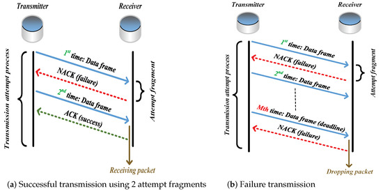
Figure 1.
Transmission attempt process using ARQ scheme.
3. Related Work
Until now, some significant studies have paid attention to analyze the MAC performance of IEEE 1901 protocol. In [21], Jung proposed a semi-Markov-based analytical model to characterize the CSMA/CA mechanism of 1901 protocol in saturated conditions. After that, Vlachou et al. put forward a series of analytical models for IEEE 1901 protocol using Renewal theory and strong law of large number (SLLN) [22,23,24,25,26], which can be used in the saturated environment. In [22,23], the authors constructed the basic analytical model and discussed the impact of deferral counter; In [24], they examined the performance tradeoff between delay and throughput; In [25], they further extended their previous work [23,24] to optimize 1901 MAC performance; Moreover, they analyzed the performance and stability of 1901 protocol under the coupling condition [26]. Similar to the work [23], Cano et al. mentioned a theoretical model for IEEE 1901 protocol in saturated conditions using renewal process theorem [27]. In [28], Hao et al. provided a unified theoretical framework for 1901 protocol, which can be used in both homogeneous and heterogeneous environment. Furthermore, they built a theoretical model for IEEE 1901 protocol in the multi-hop environment [29]. As previously said, the above-mentioned works do not consider the influence of PLC link layer’s ARQ scheme, detailed PLC channel fading type and additive non-Gaussian noise feature on the MAC performance of 1901. In addition, they fail to prove whether the proposed models have the convergence property. Table 2 summarizes the comparison between previous works and our current study for 1901 protocol analysis, containing mathematics tool and consider factors (Y denotes the considered factors, N the neglected factors).
Table 2.
Summary of the works for IEEE 1901 protocol analysis (including our current work).
4. System Model
In this part, we construct the analytical model of IEEE 1901 protocol for reliable PLC networks with ARQ scheme (the notation of essential results derived by the theoretical model is given in Table 3). For analytical tractability, we assume the reliable PLC network follows a single-hop, star-shaped topology, where all stations transmit their packets to the access point (AP). The modeling process is divided into four steps: (1) Establishing the PLC channel model to reflect the impacts of channel fading types, additive non-Gaussian noise feature and ARQ scheme on data transmission at link layer; (2) Providing a Renewal theory and Queueing dynamics-based model to depict the transmission attempt behavior of executing 1901 protocol in unsaturated environment with finite transit buffer; (3) Deriving the closed-form expressions of 1901’s MAC metrics for reliable PLC networks with ARQ scheme; (4) Proving the convergence property of our proposed analytical model (the structure of modeling steps is shown by Figure 2).
Table 3.
Notation list relevant to essential results derived by the analytical model.
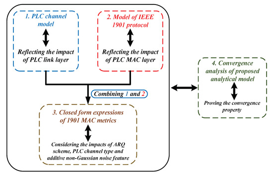
Figure 2.
Modeling steps of the proposed analytical model.
4.1. PLC Channel Model
4.1.1. Rayleigh Fading Channel
In general, a reliable PLC network employs a Rayleigh fading channel or a Log-normal fading channel [30,31]. We first consider the situation that the PLC channel follows Rayleigh fading distribution, thus the PDF (probability density function) of PLC channel gain can be written as:
where represents the channel gain with Rayleigh distribution, the scale parameter of Rayleigh distribution.
Since PLC noise contains background noise and potentially impulsive noise, following the Bernoulli-Gaussian distribution (i.e., the additive non-Gaussian noise feature) [13,34] the PDF of PLC noise distribution can be represented as
where and are the variances of the background noise and impulsive noise component, respectively; signifies the occurrence probability of the impulsive noise component. and have a ration relation, i.e., . is the ratio of the impulsive noise power.
Let be the transmission power, hence the SNR of reliable PLC networks can be expressed as:
Directly applying general communication model [13,30,31], can be expanded as , where and are two constants, X the transmission distance, and the loss exponent.
The PDF of SNR for reliable PLC networks using Rayleigh fading channel can be accordingly given by
Based on the above formal representation, we can write the CDF (Cumulative Distribution Function) of SNR using Rayleigh fading channel as
4.1.2. Log-Normal Fading Channel
Secondly, we consider the PLC channel following Log-normal fading distribution, and the PDF of PLC channel gain can be expressed as:
where denotes the channel gain with Log-normal distribution, and the scale parameters of Log-normal distribution.
On the basis, the PDF of SNR for reliable PLC networks using Log-normal fading channel can be represented as (considering the additive non-Gaussian noise feature)
where , .
Then, the CDF of SNR for reliable PLC networks using Log-normal fading channel can be derived as
where is the complimentary error function [31].
Through the above derivation, the probability that the transmission of PLC link fails, i.e., the outage probability can be expressed as
where denotes the required minimum SNR for successful decoding, i.e., threshold SNR.
4.1.3. ARQ Scheme
Since the reliable PLC network introduces ARQ scheme at link layer, one transmission attempt process is divided into several attempt fragments (no more than M fragments). Thus, for a reliable PLC network using ARQ scheme at link layer, the probability that one transmission attempt process of PLC link successes and needs x attempt fragments can be written as
Accordingly, for a reliable PLC network using ARQ scheme at link layer, the probability that one transmission attempt process of PLC link fails can be given by
4.2. The Model of IEEE 1901 Protocol
In this part, we construct the model of IEEE 1901 protocol to depict the transmission attempt behavior at MAC layer.
The model is constructed under the following assumptions:
- There are N stations transmitting their data packets over the PLC channel. The HOL (head of line) packet transmission attempt process of each station follows decoupling assumption [23].
- The transit buffer of a station is finite (denoted by K). Packets would be blocked if the transit buffer is already fully loaded (denoted by buffer blocking probability ).
- Packets arrive at the station based on Poisson process with an average arrival rate . The time of generating a packet copy is short enough and can be neglected. In addition, we assume the generating packet copy is immediately forwarded without using the transit buffer space (i.e., a packet and its copies only need 1 slot of the buffer).
4.2.1. The Transmission Attempt Probability of 1901 Protocol in Unsaturated Environment
First, we apply the results of the theoretical model established by [23] (suited for the saturated PLC environment), the transmission attempt probability of saturated environment-based 1901 protocol can be expressed using Renewal theory, i.e.,
where is the conditional collision probability of saturated environment. and denote the expected number of attempts by executing one complete procedure of IEEE 1901 protocol and the expected number of time slots spent in executing one complete procedure of 1901 (note that and are the functions of conditional collision probability). represents the expected number of time slots spent by a station at backoff stage i. signifies the probability that a station at backoff stage i must jump to the next stage (caused by unsuccessful attempt or DCP of 1901). They can be respectively represented as:
In Formula (13), r is defined as the initial selected backoff counter at stage i, h the time slots spent due to DCP of 1901. the probability of triggering DCP of 1901 and spending no more than h time slots at stage i.
Remark 1.
The detailed derivation process of , and has been shown in [23], here we do not explain anymore. In addition, we can also adopt our previous work [28] (Markov chain model) to derive .
Since we consider an unsaturated environment with finite transit buffer, the impact of buffer state should be taken into consideration. Let be the steady state probability that a station buffer is non-empty and p be the conditional collision probability in unsaturated environment, thus the transmission attempt probability of 1901 in unsaturated environment can be given by
The probability that at least one station tries to a transmission in the considered slot time, and the probability that the PLC channel is idle can be expressed respectively as:
If one of the other remaining stations attempts to transmit the HOL packet at the same slot time, a collision can be triggered (PLC networks follow the half-duplex communication mode). Hence, we construct the fixed-point equation to represent the relationship between and p, i.e.,
Remark 2.
Although we have given the expression of , is still unknown, and it relies on the size of transit buffer K and detailed packet arrival mode. Thus, in the next part, we employ Queueing dynamics to express .
4.2.2. The Derivation of Based on Queueing Dynamics
To express , we first investigate the Queueing behavior of the transit buffer. Let be the probability of a packets in the transit buffer, be the probability that there are a packets in the transit buffer after a packet departure, and be the probability that a packets arrive the station during the MAC service time [29] (the relationship between and is shown in Figure 3). Then we denote the state transition matrix as
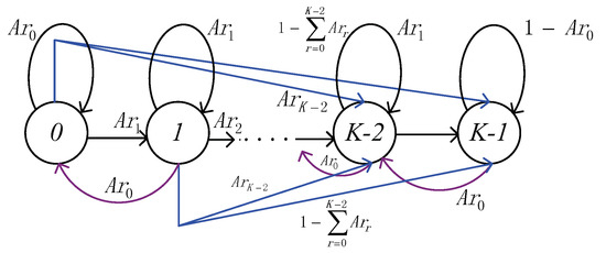
Figure 3.
The relationship between and .
Moreover, let (), we can express the relationship between and as following
Let be the expected slot time, according to the Poisson arrival feature, used in Formulas (18) and (19) can be written as ( denotes the probability that the case happens)
We further consider how to express the mean MAC service time . Applying Z transforms (i.e., Generating function method) [35,36], the generating function of initial selected backoff counter j as and can be respectively defined as:
Combining with the parameter (defined in Formulas (12) and (13)), the probability generating function (PGF) of MAC service time for reliable PLC network can be written as (for , )
Formula (23) can be expanded as
Based on the knowledge of Z transforms [35,36], we can get the arbitrary moment of by differentiating . Thus, the mean MAC service time can be expressed as
Remark 3.
in Formula (20) can be expanded as
We define the traffic intensity as , and it can be given by
Using the conclusion of queue model [37,38], the steady state probability of a packets in the transit buffer can be expressed as
Through the above derivation, the steady state probability that a station buffer is non-empty can be finally represented as
In other words, the steady state probability that a station buffer is empty equals to .
Remark 4.
Reviewing the above derivation process, is expressed as a function of and ; however, and are functions of (i.e., cannot simplified as a unary function of p), whose expression has not been obtained. It is governed not only by IEEE 1901 protocol but also by the ARQ scheme at link layer. Therefore, in the next subsection, we would combine the PLC channel model and IEEE 1901 model to derive the closed-form expressions of and other significant MAC metrics for reliable PLC networks with ARQ scheme.
4.3. The MAC Metrics of 1901 Considering ARQ Scheme
Due to the link layer’s ARQ scheme, the station can successfully transmit its HOL packet if and only if it holds the following two conditions ( and ):
: The station occupies the PLC channel through executing the 1901 protocol, and attempts to transmit its HOL packet;
: The transmit attempt process of PLC link successes.
Therefore, the successful transmission probability of reliable PLC networks can be expressed as
In Formula (30), part “I” denotes the probability of meeting condition , part “II” the probability of meeting condition . N means the successful transmission happens among one of the N stations. Furthermore, it is easy to find that has the theoretically optimal value (see the analysis in Appendix A).
Similarly, the probability that the packet is finally dropped in one transmission attempt process can be expressed as
Reviewing the ARQ scheme, one transmission attempt process can be divided into x fragments (), if the packet attempt fails in a fragment, the receiver replies a NACK frame, else an ACK frame. Thus, based on the specification of 1901 protocol [16,18], the time duration that one successful transmission needs x fragments is given by
The corresponding probability that a station successfully transmits its HOL packet and uses x fragments can be expressed as (note that )
Similarly, the time duration of “dropping packet” for a station is derived as (the time sequence is shown in Figure 4)
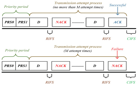
Figure 4.
1901’s time sequence for reliable PLC networks with ARQ scheme.
The time duration due to the collision is defined as
In Formula (32), (34) and (35), , , , , , D and denote the priority tone slot, response inter-frame space, contention inter-frame space, acknowledgment frame, negative acknowledgment frame, frame duration of data packet and extended inter-frame space, respectively.
Since a generic slot duration depends on whether a slot is idle or interrupted by a successful transmission or a failure transmission (“dropping packet”) or a collision, we can define as
where is the idle slot.
Thus, the expected slot time can be written as (a unary function of p)
The system throughput of reliable PLC networks with ARQ scheme S is accordingly given by
where L represents the size of data packet.
In addition, the buffer blocking probability is represented as
Through the above derivation, is finally written as a unary function of conditional collision probability p (since and are represented as the polynomials of p). Consequently, can be expanded as a polynomial of p, i.e., the right side of Formula (17) is a polynomial of p. Now we can assert that p and other significant MAC metrics are solvable in form.
4.4. Convergence Analysis of the Proposed Model
In this section, we analyze whether the proposed model has the convergence property. Since the overall analytical model needs to be solved through the fixed-point equation (Formula (17)), we should judge the convergence of the fixed point p to guarantee the proposed model’s solvability.
Reviewing Formula (17), we rewrite it as
Constructing a relaxed fixed-point sequence iteration equation [39,40] for the fixed point p, i.e.,
where represents the iteration times.
Based on the convergence theory [39,40], the sequence converges to a general fixed point p, if the first-order derivative of is bounded and .
Now we prove the above two constrained conditions hold.
Theorem 1.
The first-order-derivative of is bounded.
Lemma 1.
The first-order-derivative of is bounded.
Proof.
To degrade the difficulty of analysis, we denote by an approximate expression [38] instead of using Formula (28) (directly using Formula (28) would greatly enhance the difficulty of mathematical derivation), i.e.,
□
Taking the derivative of , we have
Recalling Formula (27), can be written as
Since is bounded (proved by Appendix B, Lemma A1 ), we can assert that is bounded. Consequently, we derive the following inequation
where (A is a positive constant).
In other words, the first-order derivative of is bounded.
Further taking the derivative of , we have
Noting that is a monotone, non-increasing function (proved by [23], Theorem 1) and (demonstrated by Appendix C, Lemma A2), thus we can get the following inequation
Hence, the first-order derivative of , i.e., is bounded.
Theorem 2.
The sequence of follows the relation of .
Proof.
We use inductive method to demonstrate this constrained condition. If holds, we can get the conclusion that .
According to Theorem 1, we have proved that the first-order derivative of is bounded, i.e., , thus can be derived as
where the “c”th line is derived based on Lagrange interpolation theorem, and is between and .
Since is continuous with respect to p, the bounded and non-increasing sequence must converge to a fixed point of p. In other words, we can guarantee that our proposed analytical model has the convergence property.□
5. Performance Evaluation
In this part, we developed simulations in Matlab. Table 1 and Table 4 provide the parameters, which would be used in simulation experiments. In the simulation, IEEE 1901 protocol is implemented by modifying the backoff counter window of 802.11 (executing backoff counter process), and adding a parallel deferral counter window (realizing the deferral counter process). In the experiment scene, a single-hop, star-shaped PLC network is constructed by N stations (adopting priority type ) and an access point (used to receive packets). The transmission distance from a station to the access point is . The self-generating packets of each station employ a Poisson process, and the average rate is . Data packets are delivered from stations to the access point through a PLC channel that follows Rayleigh fading or Log-normal fading. The additive non-Gaussian noise feature is set to be Bernoulli-Gaussian distribution, and the data packet corresponds to a frame duration D (). In addition, each simulation experiment contains 31 runs, where each run has 5000 packets for per station. The confidence interval of simulation results is ( confidence), where represents the average simulation result. We choose Fixed-Point Iteration (FPI) method [41] to solve the proposed analytical model, and the terminate precision is set as (due to the convergence property of the analytical model, using a reasonable numerical method is practicable).
Table 4.
System parameters of reliable PLC networks.
Based on 1901’s specification, two are used to declare the priority tone [28] before delivering the packet. After a , the station will receive an frame if the transmission is successful; otherwise, a frame. Between transmission attempt processes, there has a gap. If experiencing a collision, the station would wait for a duration of (corresponding to Formula (32) and Formulas (34) and (35)).
To measure the performance of IEEE 1901 protocol considering the impacts of ARQ scheme, channel fading type and additive non-Gaussian noise feature, we select four significant metrics: (1) System throughput S, (2) mean MAC service time , (3) buffer blocking probability , and (4) Successful transmission probability . The experiments totally have six groups: (1) the impact of network size, (2), the impact of packet arrival rate, (3) the impact of threshold SNR , (4) the impact of the probability of impulsive noise component , (5) the impact of the ratio of impulsive noise power , and (6) the impact of transit buffer size K. Moreover, in following figures, RF (or LNF) denotes Rayleigh fading (or Log-normal fading), Ana (or Sim) represents analysis results (or simulation results).
5.1. The Impact of Network Size N
In this simulation group, we set the threshold SNR , probability of impulsive noise component , ratio of impulsive noise power , average packet arrival rate , transit buffer size , and the number of stations N varies in . Figure 5 shows the simulation and analysis results including the system throughput S, mean MAC service time , buffer blocking probability and successful transmission probability of the reliable PLC network with different N.
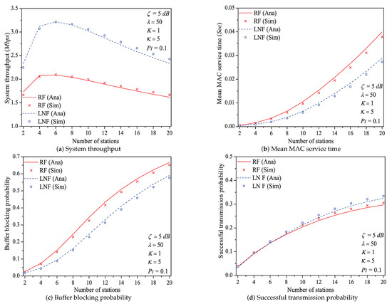
Figure 5.
The MAC performance of 1901 protocol with different N.
We can see that as the number of stations N increases, the system throughput increases first, then decreases (it is affected not only by the successful transmission probability but also by the expected slot time). With the increase of network size N. more stations would contend the medium. The data packet must wait a longer time duration to get the medium service, and the transit buffer of station is easier to be fully loaded. Consequently, the mean MAC service time and buffer blocking probability increase with the increasing network size N. As the network size has a positive influence on the performance of successful transmission probability , it increases with the increasing network size N (this conclusion can be demonstrated by Formula (30)).
Here is an example of simulation results (). the system throughput varies from to , then to under Rayleigh fading channel type; from to , then to under Log-normal fading channel type.
5.2. The Impact of Packet Arrival Rate
In this simulation group, we set the number of stations , threshold SNR , probability of impulsive noise component , ratio of impulsive noise power , transit buffer size , and the average packet arrival rate varies in . Figure 6 shows the simulation and analysis results including the system throughput S, mean MAC service time , buffer blocking probability and successful transmission probability of the reliable PLC network with different .
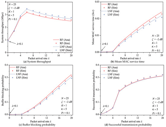
Figure 6.
The MAC performance of 1901 protocol with different .
We can see that as the packet arrival rate increases, the system throughput increases first, then slowly decreases. The mean MAC service time and buffer blocking probability increase with the increasing packet arrival rate. The reason is that as increases, the contention frequency of PLC medium is enhanced, and accordingly the collision probability increases. As a result, the data packet must wait a longer time duration to get the medium service, and the buffer of station is easier to be fully loaded. The successful transmission probability increases with the increasing . The most possible reason is that although the collision probability p and the transmission attempt probability increase with the increasing ; however, when varies in , the value of is still smaller than (reviewing the analysis in Appendix A). Thus, the part in Formula (30) is still a monotone increasing function, which accordingly results the change rule of successful transmission probability.
Here is an example of analysis results (). the system throughput varies from to , then to under Rayleigh fading channel type; from to , then to under Log-normal fading channel type.
5.3. The Impact of Threshold SNR
In this simulation group, we set the number of stations , probability of impulsive noise component , ratio of impulsive noise power , average packet arrival rate , transit buffer size , and the required threshold SNR varies in . Figure 7 shows the simulation and analysis results including the system throughput S, mean MAC service time , buffer blocking probability and successful transmission probability of the reliable PLC network with different .
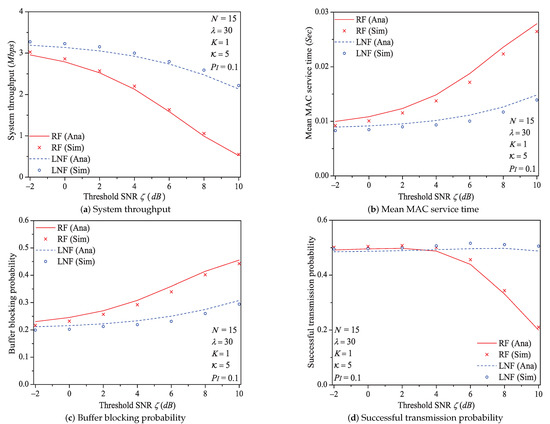
Figure 7.
The MAC performance of 1901 protocol with different ζ.
We can see that as the threshold SNR increases, the system throughput decreases. That is because as increases, the packet has a higher probability to be received in outage (the change rule of numerical values of outage probability (Formula (9)) is shown in Figure 8), in other words, the attempt fragment is easier to be unsuccessful, and the transmission efficiency is accordingly decreased. The mean MAC service time and buffer blocking probability increase with the increasing . The reason is that as increases, the station occupying PLC channel may need more attempt fragments to accomplish a successful transmission (i.e., requiring more time). Hence, the data packet must wait longer in the station, and the buffer is easier to be fully loaded. The successful transmission probability in overall decreases (not monotone), since the increasing can degrade the transmission efficiency.
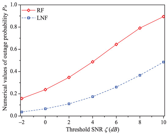
Figure 8.
The numerical values of outage probability with different .
Here is an example of simulation results (). The mean MAC service time varies from 0.0092 s to 0.0265 s under Rayleigh fading channel type; from 0.0083 s to 0.0139 s under Log-normal channel fading type.
5.4. The Impact of the Probability of Impulsive Noise Component
In this simulation group, we set the number of stations , threshold SNR dB, ratio of impulsive noise power , packet arrival rate , transit buffer size , and the probability of impulsive noise component varies in . Figure 9 shows the simulation and analysis results including the system throughput S, mean MAC service time , buffer blocking probability and successful transmission probability of the reliable PLC networks with different .
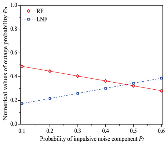
Figure 9.
The numerical values of outage probability with different .
We can see that as the probability of impulsive noise component increases, the system throughput increases under Rayleigh fading channel type, but decreases under Log-normal fading channel type. The change rules of mean MAC service time and buffer blocking probability are opposite to that of system throughput. These conclusions illustrate that the outage probability (the change rule of numerical values of is shown in Figure 10) reflecting the state of PLC link layer can greatly affect the performance of 1901 MAC metrics. Taking the example of Rayleigh fading channel type, due to the decrease of , the transmission efficiency increases, thus the system throughput increases with the increasing . At the same time, packets in the station buffer only need shorter time to get the medium service and the transit buffer is hard to be fully loaded (hence the MAC service time and buffer blocking probability decrease under Rayleigh fading channel type). The value of successful transmission probability slightly increases at first, then slightly decreases (almost unchanged). The most possible reason is that although has a relatively large change, due to the introduction of ARQ scheme, the final change extent of operator in Formula (30) is minor. For example, the numerical value of under Rayleigh fading channel type merely varies from 0.944 to 0.994 for .
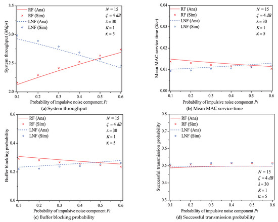
Figure 10.
The MAC performance of 1901 protocol with different PI.
Here is an example of analysis results (). The mean MAC service time varies from 0.0149 s to 0.0114 s under Rayleigh fading channel type; from 0.0102 s to 0.0130 s under Log-normal channel fading type.
5.5. The Impact of the Ratio of Impulsive Noise Power
In this simulation group, we set the number of stations , threshold SNR dB, probability of impulsive noise component , average packet arrival rate , transit buffer size , and the ratio of impulsive noise power varies in . Figure 11 shows the simulation and analysis results including the system throughput S, mean MAC service time , buffer blocking probability and successful transmission probability of the reliable PLC network with different .
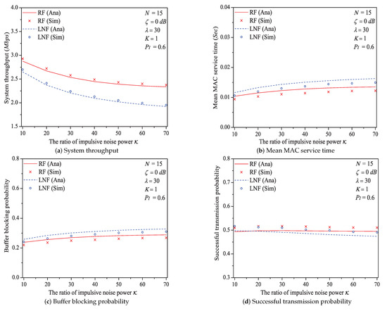
Figure 11.
The MAC performance of 1901 protocol with different .
We can see that as the ratio of impulsive noise power increases, the system throughput decreases. The reason is that as increases, the packet has a higher probability to be received in outage (the change rule of numerical values of outage probability is shown in Figure 12), in other words, the attempt fragment is easier to be unsuccessful, and the transmission efficiency is accordingly decreased. The mean MAC service time and buffer blocking probability increase with the increasing . That is because as increases, the station may need more attempt fragments to accomplish a successful transmission (i.e., requiring more time). Hence, the data packet must wait longer in the station, and the buffer is easier to be fully loaded. The successful transmission probability in overall decreases (not monotone), since the increasing can degrade the transmission efficiency.
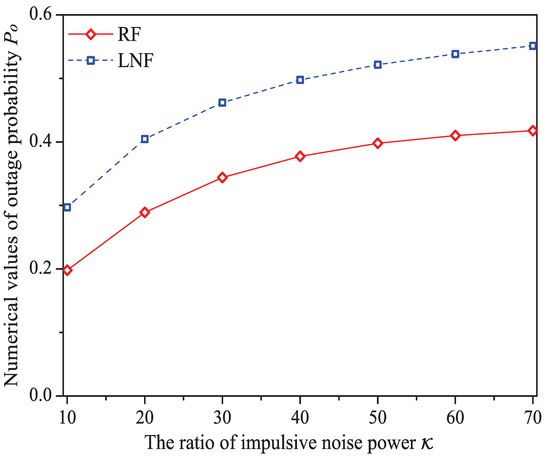
Figure 12.
The numerical values of outage probability with different .
Here is an example of simulation results (). The buffer blocking probability varies from to under Rayleigh fading channel type; from to under Log-normal channel fading type.
5.6. The Impact of Transit Buffer Size K
In this simulation group, we set the number of stations , threshold SNR dB, probability of impulsive noise component , average packet arrival rate , ratio of impulsive noise power , and the transit buffer size K varies in (the large value of K would greatly enhance the computation complexity, and the proposed analytical model needs to be solved by Lattice-Laplace method). Figure 13 shows the simulation and numerical analysis results including the system throughput S, mean MAC service time , buffer blocking probability and successful transmission probability of the reliable PLC network with different K.
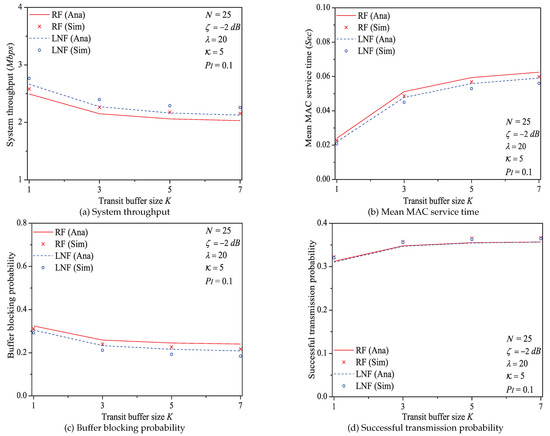
Figure 13.
The MAC performance of 1901 protocol with different K.
We can see that the performance of system throughput, mean MAC service time, buffer blocking probability, and successful transmission probability is affected by the size of transit buffer K. It is easy to find that larger size of transit buffer would nor result superior performance of system throughput and MAC service time. However, with the increase of buffer size K, the transit buffer is no longer easy to be fully loaded. Consequently, the buffer blocking probability decreases with the increasing K, and the successful transmission probability is enhanced (since more packets can enter the transit buffer rather than directly being blocked).
Here is an example of analysis results (). The buffer blocking probability varies from to under Rayleigh fading channel type; from to under Log-normal channel fading type.
Through comparing the simulation and numerical analysis results shown in Figure 5, Figure 6, Figure 7, Figure 9, Figure 11 and Figure 13, we verify that our proposed analytical model can accurately measure the MAC performance of IEEE 1901 protocol for reliable PLC networks with ARQ scheme. Since the results for priority type contain the similar rules, we do not discuss them any more in this paper. In addition, the computational complexity of solving the theoretical model (using FPI method) is , where denotes the required iteration times (the detailed analysis is given in Appendix D)
6. Conclusions
In this paper, we put forward a MAC performance analysis model of IEEE 1901 protocol for reliable PLC networks with ARQ scheme. In the modeling process, we first construct a PLC channel model to reflect the impacts of detailed channel fading type (Rayleigh fading and Log-normal fading), non-Gaussian noise feature and ARQ scheme on data transmission at PLC’s link layer. Then, we use Renewal theory and Queueing dynamics to depict the transmission attempt behavior of executing IEEE 1901 protocol in unsaturated environment with finite transit buffer. On the base of combining these two models, we derive the closed-form expressions of typical 1901 MAC metrics for reliable PLC networks with ARQ scheme. Moreover, we prove that our proposed analytical model has the convergence property. To the best of our knowledge, this should be the first work to make the performance analysis of 1901 MAC protocol for reliable PLC networks considering link layer’s ARQ scheme. Through extensive simulations, we verify that the proposed analytical model can accurately evaluate the MAC performance of 1901 protocol for reliable PLC networks with ARQ scheme. Our work provides a significant foundation for optimizing the MAC performance of reliable PLC networks, and designing reliable PLC-based IoT.
Based on this work, we can start our future study in the following research directions: (1) Analyzing the MAC performance of 1901 for reliable PLC networks, which has hidden terminals and employs other network coding schemes; (2) Designing a MAC protocol for hybrid Power-line&Visible-light communication systems; (3) Optimizing the energy consumption for energy harvesting assisted reliable PLC networks with ARQ scheme.
Author Contributions
Conceptualization, methodology, software, validation, formal analysis, investigation, resources, data curation; writing—original draft preparation, writing—review and editing, S.H.; supervision, project administration, funding acquisition, H.Z. All authors have read and agreed to the published version of the manuscript.
Funding
The work is supported by the National Natural Science Foundation of China (No.61772386) and National Key Research and Development Project (No.2018YFB1305001).
Informed Consent Statement
Informed consent was obtained from all subjects involved in the study.
Data Availability Statement
Data sharing is not applicable to this article.
Acknowledgments
The author would like to thank the editor and anonymous reviewers for helpful comments that have improved the quality of the paper.
Conflicts of Interest
The authors declare no conflict of interest.
Appendix A. The Theoretically Optimal Value of Successful Transmission Probability P suc
Let the maximum attempt fragment be . Reviewing Formula (30), it can be extended as a binary function ( is the simplified format of ), i.e.,
Thus, we take the partial derivative for
Clearly, (), has an extreme value point, i.e., , therefore, the theoretically optimal value of successful transmission probability can be written as
For , can be further expressed as
Appendix B
Lemma A1.
Is Bounded
Proof.
First, we rewrite , and it can be expressed as
Thus, we have
It is easy to find and are both monotone, increasing functions (derived by Formula (23)), thus, we only need to judge whether and are bounded.
Recalling Formula (37), we can get the following inequation
Taking the derivative of , we have
Since , we can derive the following inequation for
From the above analysis, we demonstrate that both and are bounded. Accordingly, Formula (A6) can be extended as (A denotes a positive constant)
Namely is bounded.□
Appendix C
Lemma A2.
Proof.
Directly using the conclusions proved in [23] (THEOREM 1), can be expressed as
where is denoted as
has an inequality relation derived by Formula (8) and Formula (9) of [23], i.e.,
where is expressed as
Since is a monotone, non-decreasing function [23] (THEOREM 1) and , we have
In other words, is bounded. □
Appendix D. Computation Complexity of Solving the Theoretical Model with FPI Method
To solve the numerical results of the MAC metrics, we need to calculate the correct value of p. In our paper, Fixed-Point Iteration (FPI) method is employed, and the calculation process is given as follows (Table A1):
Table A1.
Fixed-point iteration method.
Table A1.
Fixed-point iteration method.
| 1: Select any value of (0 denotes the iteration times), which are not absurd (i.e., ) | |
| 2: Calculate the values of , and in order (based on our theoretical model) | |
| 3: Find out the value of through using Formula (14) based on step 2’s conclusion | |
| 4: Derive the new by substituting into Formula (17) | |
| 5: Repeat the above process (through iterating calculation) | |
| 6: If ( is the terminate precision we defined), replace p with , and then calculate the numerical values of other MAC metrics. |

Figure A1.
The relationship between iteration times and convergence precision under the impact of transit buffer size K.
Figure A1.
The relationship between iteration times and convergence precision under the impact of transit buffer size K.

Clearly, if we set a reasonable , we can finally derive the results of the theoretical model in a finite number of iteration times IT (a constant). Since we have assumed that the transmission attempt process of each station follows the decoupling assumption [23], the computational complexity of solving our theoretical model can be written as
It should be noted that the number of iteration times is affected by the system parameters setting. Here we give an example. Figure A1 shows the relationship between iteration times of solving the proposed theoretical model and the convergence precision (equal to ) for the last experiment group (“impact of transit buffer size K”). We can find that the iteration times and the buffer size have a positive relationship, in other words, the large value of buffer size K would enhance the iteration times (decreasing the convergence speed). The reason is that the large buffer would enhance the random matrix’s dimension given by Formulas (18) and (19).
References
- Sandell, M.; Raza, U. Application Layer Coding for IoT: Benefits, Limitations, and Implementation Aspects. IEEE Syst. J. 2019, 13, 554–561. [Google Scholar] [CrossRef]
- Ramon, S.I.; Maria-Dolores, C. State of the Art in LP-WAN Solutions for Industrial IoT Services. Sensors 2016, 16, 708. [Google Scholar]
- Gubbi, J.; Buyya, R.; Marusic, S.; Palaniswamia, M. Internet of Things (IoT): A Vision, Architectural Elements, and Future Directions. Future Gener. Comput. Syst. 2013, 29, 1645–1660. [Google Scholar] [CrossRef]
- Jani, M.; Garg, P.; Gupta, A. On the Performance of a Cooperative PLC-VLC Indoor Broadcasting System Consisting of Mobile User Nodes for IoT Networks. IEEE Trans. Broadcast. 2020, 1–10. [Google Scholar] [CrossRef]
- Pavlidou, N.; Vinck, A.J.H.; Yazdani, J.; Honary, B. Power line communications: State of the art and future trends. IEEE Commun. Mag. 2003, 41, 34–40. [Google Scholar] [CrossRef]
- Son, Y.S.; Pulkkinen, T.; Moon, K.D.; Kim, C. Home energy management system based on power line communication. IEEE Trans. Consum. Electron. 2010, 56, 1380–1386. [Google Scholar] [CrossRef]
- Carcangiu, S.; Fanni, A.; Montisci, A. A Optimization of a power line communication system to manage electric vehicle charging stations in a smart grid. Energies 2019, 12, 1767. [Google Scholar] [CrossRef]
- Cano, C.; Pittolo, A.; Malone, D.; Lampe, L.; Tonello, A.M.; Babak, A.G. State of the Art in Power Line Communications: From the Applications to the Medium. IEEE J. Sel. Areas Commun. 2016, 34, 1935–1952. [Google Scholar] [CrossRef]
- Sharma, K.; Saini, L.M. Power-line communications for smart grid: Progress, challenges, opportunities and status. Renew. Sustain. Energy Rev. 2017, 67, 704–751. [Google Scholar] [CrossRef]
- Bilbao, J.; Crespo, P.M.; Armendariz, I.; Medard, M. Network Coding in the Link Layer for Reliable Narrowband Powerline Communications. IEEE J. Sel. Areas Commun. 2016, 34, 1965–1977. [Google Scholar] [CrossRef]
- Papaioannou, A.; Papadopoulos, G.D.; Pavlidou, F.N. Hybrid ARQ Combined With Distributed Packet Space-Time Block Coding for Multicast Power-Line Communications. IEEE Trans. Power Deliv. 2008, 23, 1911–1917. [Google Scholar] [CrossRef]
- Makki, B.; Amat, A.G.i.; Eriksson, T. Green Communication via Power-optimized HARQ Protocols. IEEE Trans. Veh. Technol. 2014, 63, 161–177. [Google Scholar] [CrossRef]
- Mathur, A.; Ai, Y.; Cheffena, M.; Bhatnagar, M.R. Performance of Hybrid ARQ over Power Line Communications Channels. In Proceedings of the 2020 IEEE 91st Vehicular Technology Conference (VTC2020-Spring), Belgium, Belgium, 25–28 May 2020. [Google Scholar]
- Sakunnithimetha, N.; Tuntoolavest, U. An efficient new ARQ strategy for vector symbol decoding with performance in power line communications. In Proceedings of the 2017 International Electrical Engineering Congress, Pattaya, Thailand, 8–10 March 2017. [Google Scholar]
- Tsokalo, I.; Gabriel, F.; Pandi, S.; Fitzek, F.H.P.; Lehnert, R. Reliable feedback mechanisms for routing protocols with network coding. In Proceedings of the 2018 IEEE International Symposium on Power Line Communications and its Applications (ISPLC), Manchester, UK, 8–11 April 2018. [Google Scholar]
- IEEE. IEEE Standard for Broadband over Power Line Networks: Medium Access Control and Physical Layer Specifications; IEEE Std 1901–2010; IEEE: Piscataway, PA, USA, 2010; Volume 10, pp. 1–1589. [Google Scholar]
- Homeplug Alliance. Available online: www.homeplug.org (accessed on 12 June 2016).
- IEEE 1901 HD-PLC (High Definition Power Line Communication). Available online: www.hd-plc.org (accessed on 6 February 2018).
- de Oliveira, R.M.; Vieira, A.B.; Latchman, H.A.; Ribeiro, M.V. Medium access control Pprotocols for Power line communication: A Survey. IEEE Commun. Surv. Tutorials 2019, 2, 920–939. [Google Scholar] [CrossRef]
- Hao, S.; Zhang, H.Y. An energy harvesting modified MAC protocol for power-line communication systems using RF energy transfer: Design and analysis. IEICE Trans. Commun. 2020, E103-B. [Google Scholar] [CrossRef]
- Jung, M.H.; Chung, M.Y.; Lee, T.J. MAC throughput analysis of HomePlug1.0. IEEE Commun. Lett. 2005, 9, 184–186. [Google Scholar] [CrossRef]
- Vlachou, C.; Banchs, A.; Herzen, J.; Thiran, P. Performance analysis of mac for power-line communications. In Proceedings of the SIGMETRICS 2014, Austin, TX, USA, 16–20 June 2014; pp. 585–586. [Google Scholar]
- Vlachou, C.; Banchs, A.; Herzen, J.; Thiran, P. Analyzing and boosting the performance of power-line communication networks. In Proceedings of the 10th International on Conference on Emerging Networking Experiments and Technologies, CoNEXT 2014, Sydney, Australia, 2–5 December 2014; pp. 1–12. [Google Scholar]
- Vlachou, C.; Banchs, A.; Herzen, J.; Thiran, P. On the MAC for Power-Line Communications: Modeling Assumptions and Performance Tradeoffs. Semiotica 2014, 2007, 97–104. [Google Scholar]
- Vlachou, C.; Banchs, A.; Salvador, P. Analysis and enhancement of CSMA/CA with deferral in power-line communications. IEEE J. Sel. Areas Commun. 2016, 34, 1978–1991. [Google Scholar] [CrossRef]
- Vlachou, C.; Banchs, A.; Herzen, J.; Thiran, P. How CSMA/CA with deferral affects performance and dynamics in power-line communications. IEEE/ACM Trans. Netw. 2017, 25, 250–263. [Google Scholar] [CrossRef]
- Cano, C.; Malone, D. On Efficiency and Validity of Previous Homeplug MAC Performance Analysis. Comput. Netw. 2016, 83, 118–135. [Google Scholar] [CrossRef]
- Hao, S.; Zhang, H.Y. From homogeneous to heterogeneous: An analytical model for IEEE 1901 power line communication networks in unsaturated conditions. IEICE Trans. Commun. 2019, E102-B, 1636–1648. [Google Scholar] [CrossRef]
- Hao, S.; Zhang, H.Y. Theoretical modeling for performance analysis of IEEE 1901 power-line communication networks in the multi-hop environment. J. Supercomput. 2020, 76, 2715–2747. [Google Scholar] [CrossRef]
- Neelima, A.; Kumar, S.P. Error performance of hybrid wireless-power line communication system. AEU—Int. J. Electron. Commun. 2018, 95, 242–248. [Google Scholar]
- Kolade, O.; Familua, A.D.; Cheng, L. Indoor amplify-and-forward power-line and visible light communication channel model based on a semi-hidden markov model. AEU–Int. J. Electron. Commun. 2020, 124, 1–9. [Google Scholar] [CrossRef]
- Agrawal, N.; Sharma, P.K.; Tsiftsis, T.A. Multihop DF Relaying in NB-PLC System Over Rayleigh Fading and Bernoulli-Laplacian Noise. IEEE Syst. J. 2019, 13, 357–364. [Google Scholar] [CrossRef]
- Jani, M.; Garg, P.; Gupta, A. Performance Analysis of a Mixed Cooperative PLC-VLC System for Indoor Communication Systems. IEEE Syst. J. 2020, 14, 469–476. [Google Scholar] [CrossRef]
- Manav, A.; Bhatnagar, M.R.; Panigrahi, B.K. PLC performance evaluation with channel gain and additive noise over nonuniform background noise phase. Eur. Trans. Telecommun. 2017, 28, e3131. [Google Scholar]
- EliahuIbrahim. Theory and Application of the Z-Transform Method; Wiley: Hoboken, NJ, USA, 1964. [Google Scholar]
- Graf, U. Applied Laplace-And Z-Transforms; Springer: New York, NY, USA, 2004. [Google Scholar]
- Bolch, G.; Greiner, S.; Meer, H.D.; Trivedi, K.S. Queuing Networks and Markov Chains; Wiley: Hoboken, NJ, USA, 1998. [Google Scholar]
- Saloff-Coste, L. Lectures on Finite Markov Chains; Springer: Berlin/Heidelberg, Germany, 1997. [Google Scholar]
- Iglehart; Donald, L. Weak convergence in queueing theory. Adv. Appl. Probab. 1973, 5, 570–594. [Google Scholar] [CrossRef]
- Billingsley, P. Convergence of Probability Measures; Wiley: Hoboken, NJ, USA, 1968. [Google Scholar]
- Hamming, R.W. Numerical Methods for Scientists and Engineers; Dover Publications: St. Mineola, NY, USA, 1973. [Google Scholar]


Publisher’s Note: MDPI stays neutral with regard to jurisdictional claims in published maps and institutional affiliations. |
© 2020 by the authors. Licensee MDPI, Basel, Switzerland. This article is an open access article distributed under the terms and conditions of the Creative Commons Attribution (CC BY) license (http://creativecommons.org/licenses/by/4.0/).