Robust Time-Delay Feedback Control of Vehicular CACC Systems with Uncertain Dynamics

Abstract

This paper proposes a new, robust time-delay cooperative adaptive cruise control (CACC) approach for vehicle platooning systems with uncertain dynamics and varying communication delay. The uncertain CACC models with perturbed parameters are used to describe the uncertain dynamics of the vehicle platooning system. By combining the constant time headway strategy and predecessor-following communication topology, a set of robust delay feedback controllers is designed for the uncertain vehicle platoon with varying communication delay. Then, the set of CACC controllers is computed by solving some linear matrix inequalities, which further establish the robust (string) stability of the uncertain platooning system with the varying communication delay. The co-simulation experiment of CarSim and Simulink with a group of a seven-car platoons and varying velocity is used to demonstrate the effectiveness of the presented method.

1. Introduction

Recently, cooperative adaptive cruise control of a group of connected and automated vehicles (CAVs) has attracted considerable attention in both industrial and academic communities. With the information exchange among vehicles in the group by vehicle-to-anything (V2X) communication [1], CACC systems can improve traffic flow stability, throughput, driving safety and ride comfort of vehicles [2,3]. CACC technology is now shown to be one of the promising intelligent transportation system technologies [2,3,4,5,6,7,8,9].

The main objective of CACC is to adjust the group of CAVs to form a vehicle platoon with keeping a desired safe inter-vehicle distance, i.e., spacing. Besides the stability issue of CACC systems, the string stability of vehicle platoons [2,3] is the key aim of theoretical analysis of the vehicular CACC system. The string stability property of vehicle platoons implies that the perturbation from the leading vehicle of a platoon will not be amplified downstream through the platoon [2,3]. This property can effectively avoid a halt or collision at the end of a platoon [10,11]. Various CACC methods have been proposed to derive the (string) stability of vehicle platoons (e.g., see [5,6,7,8,9,12,13,14,15,16,17,18] and the references therein).

In CACC systems, the real-time behaviors of front vehicles are dispatched to the nearest following vehicles by the V2X wireless network. Hence, the V2X network has important effects on the (string) stability of vehicular CACC systems due to varying communication delays [3]. Many efforts addressed these effects within the networked control systems framework [19,20,21,22,23,24,25]. For instance, the effect of network-induced constant delays or sample-and-hold devices on string stability was studied within a networked control system perspective [19]. By using the Smith predictor [26], which is known to be robust against time-delay, a model-based robust H_∞ control was presented for a granulation process with reference updating [27]. The most results on CACC were derived by assuming constant time-delay of the V2X network and few results have been obtained to deal with varying heterogeneous communication delay. For instance, the author in [24] proposed a distributed consensus strategy for control of the vehicle platoon represented by second order integral systems with varying heterogeneous communication delay. In the previous work [25], we designed CACC controllers for nominal vehicle platoon systems, i.e., the CACC systems are assumed to be modelled exactly. However, in actual it is hard to derive an exactly CACC model for a real CACC system. Moreover, the unknown dynamics of a CACC system will degrade the controllers based on the nominal CACC system. Here the CACC controllers in [25] will be generalized as robust CACC controllers by taking into account the uncertain dynamics of CACC systems.

In most of the existing CACC methods, the dynamic models and parameters of systems are assumed be partially or fully known for design of CACC controllers. The assumption may degrade closed-loop performance in the face of parametric uncertainties and/or unknown disturbances. Compared to a lot of nominal CACC results, fewer work considered the model uncertainties in CACC systems. For example, in [28], an adaptive optimal control strategy was proposed for heterogeneous CACC system with uncertain dynamics by resorting adaptive dynamic programming. The authors in [29] presented a robust distributed control protocols for vehicle platoons with unknown nonlinear dynamics under both the predecessor-following and the bidirectional control configurations. Considering parametric uncertainties and uniform communication delay, in [30], the robust H_∞ control method was introduced for vehicle platoons with fully networked bidirectional control structure and the constant distance headway strategy. It remains challenging to understand how the combination of uncertain dynamics and heterogeneous communication delay affects the cooperative cruise control of vehicle platoons.

The aim of this paper is to solve robust CACC problems in the networked control framework by taking into account parametric uncertainties and heterogeneous communication delay. By adopting the constant time headway strategy and predecessor-following communication topology, the vehicular CACC systems with uncertain dynamics and heterogeneous communication delay are modeled as a family of uncertain car-following models with perturbed parameters and varying time-delay. Then, a set of robust delay feedback controllers is designed for the uncertain vehicle platoon with varying communication delay and is computed in such way that each vehicle evaluates its own controller using only neighborhood information. Moreover, the platoon formation and its stability are guaranteed in the presence of parametric uncertainties and varying time-delay by some linear matrix inequalities (LMI) conditions. With respect to the constant distance headway strategy, here, the car-following models consider the constant time headway which enables a vehicle to proportionally adjust to the desired spacing based on its velocity [2,3,4]. Hence, the used models are more appropriate in the real-world applications. Finally, numerical results of co-simulation experiments of CarSim and Simulink illustrate the effectiveness of the proposed CACC method for string stability of a seven-vehicle platoon in the varying speed scenario.

Notations: Throughout the paper, P > 0 means that the matrix P is positive definite and diag{...} denotes a block-diagonal matrix. The symbol I denotes the identity matrix with compatible dimensions and traditional symbol ‘T’ denotes the transpose of a vector or a matrix. The symmetric terms in a symmetric matrix are denoted by ‘*’, e.g., $\left[\begin{array}{cc}M& N\\ *& L\end{array}\right]=\left[\begin{array}{cc}M& N\\ N^{\mathrm{T}}& L\end{array}\right]$.

2. Problem Formulation

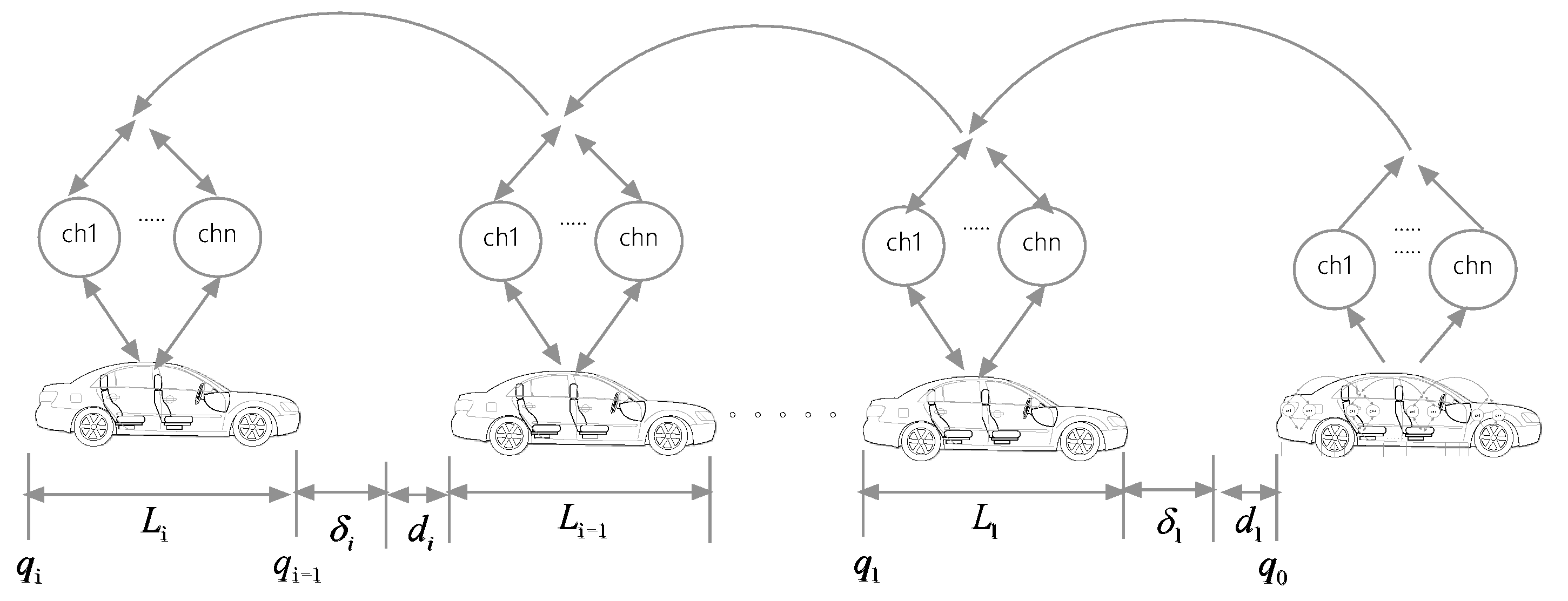
Consider a group string of N + 1 vehicles moving along a single lane and assume that they run in horizontal environment (see Figure 1), where the first vehicle in the platoon presents the reference trajectory of the string according to some safety spacing policies. In this platoon, each vehicle shares its acceleration with the following vehicles through a predecessor-following (PF) communication network consisting of multiple redundant channels. Due to using multi-channel transmission, here we assume that the network has no packet loss but may exist communication delay for CACC of the vehicle platoon. The vehicles are also equipped with onboard sensors to measure the inter-vehicle distance and relative velocity with respect to its preceding vehicle.

Consider the vehicle platoon in Figure 1 and let L_i, q_i, v_i and a_i be the length, position, velocity and acceleration of the ith vehicle in the platoon for i = 0,1,…,N, where i = 0 stands for the leading vehicle. In this figure, δ_i is the spacing error and chj stands for the jth wireless channel for j = 1,…,n. For the ith vehicle in the platoon, the longitudinal dynamics can be described by [7,17]

$${\dot{q}}_i(t)=v_i(t),\hspace{1em}{\dot{v}}_i(t)=a_i(t),\hspace{1em}{\dot{a}}_i(t)=f_i(v_i(t),a_i(t))+g_i(v_i(t)){\vartheta }_i(t),\hspace{1em}\forall t\ge 0$$

(1)

where ϑ_i(t) is the engine input of the ith vehicle at time t ≥ 0, and functions f_i and g_i are given by

$$\begin{array}{l}{f}_i\left(v_i,a_i\right)=-\frac{1}{{\varsigma }_i}\left(a_i+\frac{\sigma Y_i{f}_{di}}{2m_i}{v}_i^2+\frac{p_{mi}}{m_i}\right)-\frac{\sigma Y_i{f}_{di}{v}_i{a}_i}{m_i}\\ g_i\left(v_i\right)=\frac{1}{{\varsigma }_i{m}_i}\end{array}$$

where ς_i is the internal actuator dynamics of the vehicle in tracking any desired acceleration command, σ is the air density, and Y_i, f_di, p_mi and m_i are the cross-sectional area, drag coefficient, mechanical drag and mass of the vehicle, respectively. In order to linearize the acceleration equation in Equation (1), the following equation is used [17]:

$${\vartheta }_i=u_i{m}_i+\sigma Y_i{f}_{di}{v}_i^2/2+p_{mi}+{\zeta }_i\sigma Y_i{f}_{di}{v}_i{a}_i$$

(2)

where the new control u_i is the desired acceleration command of vehicle i. Substituting Equation (2) into the third equation in Equation (1), we obtain a three-order linearized model that is used to represent the longitudinal dynamics of the vehicle [19], i.e.,

$${\dot{q}}_i(t)=v_i(t),\hspace{1em}{\dot{v}}_i(t)=a_i(t),\hspace{1em}{\dot{a}}_i(t)=-1/{\varsigma }_i{a}_i+1/{\varsigma }_i{u}_i.$$

(3)

The model simplifies the complexity of modeling the longitudinal dynamics of vehicles. It has been shown that the linear model (1) adequately describes the longitudinal dynamics of the acceleration- controlled vehicles via the experimental validation and has been widely used to design CACC controllers of various vehicle platoons [19].

Note that the linear model equation (3) can be viewed as the upper layer cruise control systems in the double layers hierarchical control structure used widely by CACC systems, e.g., [7,10,19]. In this control structure, the nonlinear equations in Equation (2) are seen as the lower layer controllers of vehicles and are generally assumed to be perfectly designed in CACC systems although the aerodynamics drag force (0.5σY_if_div²) is usually hard to estimate perfectly due to unknown coefficients of drag [17,21]. In this paper, we focus ourselves on the upper layer cruise control systems in Equation (3) by assuming the desired control performance of the lower layer controllers of vehicles.

Let the actual inter-vehicle distance of vehicle i be d_i = q_i−1 − q_i − L_i, where q_i−1 is the position of its predecessor. In order to regulate the inter-vehicle distance d_i to a small desired spacing, the constant time headway strategy is adopted as the safe spacing policy of the proposed CACC system, i.e.,

$$d_{r,i}(t)=D_i+T_i{v}_i(t)$$

(4)

where d_r,i is the desired spacing between vehicles i and i − 1, D_i is the desired safety inter-vehicle distance at standstill, v_i is the velocity and T_i is the time gap of vehicle i. The difference between actual and desired inter-vehicle distances defines the car-following error of each vehicle i as e_i = d_i − d_r,I = q_i−1− q_i − L_i − d_r,i. In this study, the vehicle platoon moves with a referred varying velocity, namely, the leading vehicle satisfies that $a_0(t)={\dot{v}}_0(t)\ne 0$.

In order to model the longitudinal CACC system of the vehicle platoon in Figure 1, the error state vector of the ith vehicle is selected as x_i = [e_i Δv_i a_i]^T, where Δv_i is the relative velocity between the ith-pair adjacent vehicles. Then from Equations (3) and (4), the dynamics of the error variables for the vehicle can be represented as

$${\dot{x}}_i(t)=(A_i+\mathrm{\Delta }{A}_i(t))x_i(t)+(B_i+\mathrm{\Delta }{B}_i(t))u_i(t)+G_i{x}_{i-1}(t)$$

(5)

where matrices

$$A_i=\left[\begin{array}{ccc}0& 1& -T_i\\ 0& 0& -1\\ 0& 0& -1/{\varsigma }_i\end{array}\right], B_i=\left[\begin{array}{c}0\\ 0\\ 1/{\varsigma }_i\end{array}\right], G_i=\left[\begin{array}{ccc}0& 0& 0\\ 0& 0& 1\\ 0& 0& 0\end{array}\right]$$

for i = 1,…,N and uncertainties ΔA_i and ΔB_i are the unknown parameter perturbations of the model. Note that these parameter perturbations may be caused by uncertain internal dynamics of vehicles and/or uncertain driving conditions [17,21]. Here, matrices ΔA_i and ΔB_i are real-valued matrix functions and can represent time-varying parameter uncertainties of the CACC system of the vehicle platoon. Moreover, the time-varying parameter uncertainties satisfy structural uncertainties

$$\left[\begin{array}{cc}\mathrm{\Delta }{A}_i(t)& \mathrm{\Delta }{B}_i\end{array}(t)\right]=D_i{F}_i(t)\left[\begin{array}{cc}{E}_{i,1}& E_{i,2}\end{array}\right]$$

(6)

for all time t ≥ 0, where D_i, E_i,1, and E_i,2 are constant matrices with appropriate dimensions and F_i(t) is an unknown matrix function with associated dimension and satisfies that [17]

$$F_i{}^T(t)F_i(t)\le I,\hspace{1em}\forall t\ge 0.$$

(7)

Then, by using Equation (7), the uncertainties ΔA_i and ΔB_i are described by a set of unknown matrix functions F_i. Since the ith vehicle receives the signals transmitted by onboard sensors and V2X communication, respectively, the output of the vehicle in the platoon is defined as

$$y_i(t)={\left[\begin{array}{cc}{x}_i^T(t)& a_{i-1}(t-{\tau }_i(t))\end{array}\right]}^T$$

(8)

where τ_i is the unavoidable varying communication delay. Typically, τ_i is ranged over some finite time intervals and can be assumed bounded by some a maximum value, i.e., 0 ≤τ_I ≤h with the upper bound h > 0. In dedicated short-range communication (DSRC), the magnitude of h is reported as 0.1–0.4 s [21].

In [25], we proposed a time-delay feedback CACC approach for nominal vehicle platoon systems, i.e., the longitudinal CACC system in Equation (5) is free to be subject to uncertainties ΔA_i and ΔB_i. However, in practical there always exit some unknown uncertainties of vehicle platoon systems due to e.g. uncertain internal dynamics of vehicles and/or uncertain driving conditions [17,21]. Hence, the goal of this paper is to design CACC controllers for the system in Equation (5) such that the controllers regulate the inter-vehicle distance d_i to the desired safe spacing d_r as well as maintaining string stability of the vehicle platoon in the presence of some unknown uncertainties and varying delays. To this end, the robust time-delay feedback CACC controller for the ith vehicle in the platoon

$$u_i(t)=K_i{y}_i(t)=k_{i,1}{e}_i(t)+k_{i,2}\mathrm{\Delta }{v}_i(t)+k_{i,3}{a}_i(t)+k_{i,4}{a}_{i-1}(t-{\tau }_i(t))$$

(9)

is designed such that the state x_i of uncertain system in Equation (5) is regulated to zero in the presence of uncertainties in Equation (6) and varying delays τ_i(t), as well as guaranteeing string stability of the uncertain vehicle platoon in Equation (5), where the gain vector K_i = [k_i,1, k_i,2, k_i,3, k_i,4] will be determined in the next section. In what follows, some concepts are defined before the design of the CACC controller.

Definition 1.

(Robust stability). The uncertain CACC system in Equation (5)–Equation (6) with Equation (9) is robust stable if for a step change of referred speed at time t = 0, the system in Equation (5) is stabilized by the CACC controller in Equation (9) to the origin in the presence of uncertainties in Equation (6).

Definition 2.

(Robust string stability). A vehicle platoon with the uncertain CACC system in Equation(5)–Equation(6) with Equation(9) is robust string stable if the CACC system is robust stable and the inequality ‖G_i(jw)‖ ≤ 1 holds for any w ≥ 0, where G_i(s) = a_i(s)/a_i−1(s), and a_i(s) and a_i−1(s) are the Laplace transforms of a_i(t) and a_i−1(t), respectively.

Note that robust string stability is an extension of string stability from nominal to uncertain platooning systems. String stability of a vehicle platoon implies that the oscillations do not amplify downstream along the platoon, which are resulted from any maneuver of leading vehicle. Hence, string stability can be seen as a measurement on the amplification of perturbations along the vehicle string. When the onboard sensors and wireless V2X work in a normal situation, the vehicle platoon with a CACC system is string stable under some well accepted conditions, e.g., [2,3,11]. However, due to the uncertainties and the varying communication delay, the vehicle platoon with a CACC system is getting to an uncertain system subject to varying time-delay. This makes the robust CACC problem rather challenging.

3. Robust CACC of Vehicle Platoons

In this section, the robust controller in Equation (9) is designed to achieve the robust stability of the system in Equation (5) in the presence of uncertainties in Equation (6) and varying communication delay.

3.1. Closed-Loop Uncertain CACC Systems

The closed-loop CACC system is obtained by combining the dynamics of error states in Equation (5) with the CACC controller in Equation (9). To this end, this CACC controller is firstly rewritten as

$$\begin{array}{l}{u}_i(t)=K_i{\left[\begin{array}{cc}{x}_i^{\mathrm{T}}(t)& a_{i-1}(t-{\tau }_i(t))\end{array}\right]}^{\mathrm{T}}\\ \hspace{1em}\hspace{1em}\underset{¯}{\underset{¯}{\mathrm{\Delta }}} K_{i,1}{x}_i(t)+K_{i,2}\begin{array}{ccc}[0& 0& 1\end{array}]x_{i-1}(t-{\tau }_i(t))\end{array}$$

(10)

where K_i,1 = [k_i,1 k_i,2 k_i,3] and K_i,2 = k_i,4, which will be computed elaborately in Section 3.2, the symbol “$\underset{¯}{\underset{¯}{\mathrm{\Delta }}}$” represents "defined as". Then applying the CACC controller in Equation (10) into the system in Equation (5), we have the closed-loop uncertain CACC system of the ith vehicle

$$\begin{array}{l}{\dot{x}}_i(t)=(A_i+\mathrm{\Delta }{A}_i+B_i{K}_{i,1}+\mathrm{\Delta }{B}_i{K}_{i,1})x_i(t)+G_i{x}_{i-1}(t)\\ \hspace{0.33em}\hspace{0.33em}\hspace{1em}\hspace{1em}+(B_i+\mathrm{\Delta }{B}_i)K_{i,2}\left[\begin{array}{ccc}0& 0& 1\end{array}\right]x_{i-1}(t-{\tau }_i(t))\end{array}$$

(11)

Let x = [x₁^T x₂^T⋯⋯x_N^T]^T. From Equation (11), the closed-loop uncertain CACC system of the whole vehicle platoon can be re-written in a compact form of

$$\begin{array}{ll}\dot{x}(t)=& (A+\mathrm{\Delta }A+B{K}_1+\mathrm{\Delta }B{K}_1)x(t)\\ & +(\overline{B}+\mathrm{\Delta }\overline{B})K_2{Y}_{1}x(t-\tau (t))\\ & +G{x}_0(t)+{\overline{B}}_1{K}_{1,2}\left[\begin{array}{ccc}0& 0& 1\end{array}\right]x_0(t-{\tau }_1)\end{array}$$

(12)

with matrices

$$A=\left[\begin{array}{cccc}{A}_1& 0& \cdots & 0\\ G_2& A_2& \cdots & 0\\ \cdots & \ddots & \ddots & \cdots \\ 0& \cdots & G_N& A_N\end{array}\right],\hspace{0.33em}\hspace{0.33em}\overline{B}=\left[\begin{array}{cccc}0& 0& \cdots & 0\\ B_2& 0& \cdots & 0\\ \cdots & \ddots & \ddots & \cdots \\ 0& \cdots & B_N& 0\end{array}\right],\hspace{0.33em}\hspace{0.33em}\mathrm{\Delta }\overline{B}=\left[\begin{array}{cccc}0& 0& \cdots & 0\\ \mathrm{\Delta }{B}_2& 0& \cdots & 0\\ \cdots & \ddots & \ddots & \cdots \\ 0& \cdots & \mathrm{\Delta }{B}_N& 0\end{array}\right],$$

ΔA = diag{ΔA₁,ΔA₂,…,ΔA_N}, B = diag{B₁,B₂,…,B_N}, ΔB = diag{ΔB₁,ΔB₂,…,ΔB_N}, K₁ = diag{K_1,1, K_2,1,…,K_N,1}, K₂ = diag{K_2,2,K_3,2,…,K_N,2,0}, Y₁ = diag{[0 0 1]₂, [0 0 1]₃,…,[0 0 1]_N, 0}, G = [G₁^T,0,…,0]^T, ${\overline{B}}_1=$ [B₁^T+ΔB₁^T,0,…,0]^T and τ = {τ₁,τ₂,..,τ_N}. Moreover, substituting Equation (6) into Equation (12), it is obtained that

$$\begin{array}{ll}\dot{x}(t)=& (A+DF(t)E_1+B{K}_1+DF(t)E_2{K}_1)x(t)\\ & +(\overline{B}+R_{1}DF(t)E_2{R}_2)K_2{Y}_{1}x(t-\tau (t))\\ & +G{x}_0(t)+{\overline{B}}_1{K}_{1,2}\left[\begin{array}{ccc}0& 0& 1\end{array}\right]x_0(t-{\tau }_1)\end{array}$$

(13)

with matrices D = diag{D₁,D₂,…,D_N}, E₁ = diag{E_1,1,E_2,1,…,E_N,1}, E₂ = diag{E_1,2,E_2,2,…,E_N,2}, F(t) = diag{F₁(t), F₂(t),…,F_N(t)},

$$R_1={\left[\begin{array}{cccc}0& 0& \cdots & 0\\ 0& I_N& \cdots & 0\\ \cdots & \ddots & \ddots & \cdots \\ 0& \cdots & 0& I_N\end{array}\right]}_{N\times N},\hspace{0.33em}\hspace{0.33em}{R}_2={\left[\begin{array}{cccc}0& 0& \cdots & 0\\ 1& 0& \cdots & 0\\ \cdots & \ddots & \ddots & \cdots \\ 0& \cdots & 1& 0\end{array}\right]}_{N\times N}$$

3.2. Controller Design

Consider the closed-loop uncertain CACC system in Equation (13) and let A_k = A + DF(t)E₁ + BK₁ + DF(t)E₂K₁ and $B_k=\overline{B}{K}_2{Y}_1+R_{1}DF(t)E_2{R}_2{K}_2{Y}_1$ for simplicity. Then the closed-loop system in Equation (13) is equal to

$$\dot{x}(t)=A_{k}x(t)+B_{k}x(t-\tau (t))$$

(14)

In what follows, some known lemmas are introduced to derive the robust stability of the uncertain CACC system.

Lemma 1.

[31]. Let P_i, Q_i and R_i be any positive-definite symmetric matrices with appropriate dimensions for i = 1 and 2. Then there exists a symmetric matrix M such that

$$\left[\begin{array}{cc}{P}_1-M& Q_1\\ Q_1^{\mathrm{T}}& R_1\end{array}\right]>0,\hspace{1em}\left[\begin{array}{cc}{P}_2+M& Q_2\\ Q_2^{\mathrm{T}}& R_2\end{array}\right]>0$$

(15)

if and only if

$$\left[\begin{array}{ccc}{P}_2+P_2& Q_1& Q_2\\ *& R_1& 0\\ *& *& R_2\end{array}\right]>0$$

(16)

Lemma 2.

[32]. Given any matrices Q = Q^T, H and E with appropriate dimensions, the matrix inequality $Q+HF(t)E+E^{T}F{(t)}^T{H}^T<0$ holds for the matrix F(t) in inequality Equation (7) if and only if there exists a number ε > 0 such that the matrix inequality $Q+{\epsilon }^{-1}H{H}^T+\epsilon E^{T}E<0$ is true.

Now the robust stability of the uncertain CACC system in Equation (5) of the vehicle platoon subject to the parameter uncertainties in Equation (6) and time-varying delay is summarized as the following theorem.

Theorem 1.

Consider the uncertain closed-loop CACC system in Equation (13). If there exist two positive definite symmetric matrices P∈^3N×3N and R∈^3N×3N such that the following nonlinear matrix inequality holds:

$$\mathsf{\Phi }=\left[\begin{array}{ccc}{M}_{11}& M_{12}^{\mathrm{T}}& M_{13}^{\mathrm{T}}\\ *& -h{R}^{-1}& 0\\ *& *& -hR\end{array}\right]<0$$

(17)

where matrices$M_{11}=\left[\begin{array}{cc}\vartheta & P{B}_k-N_1^{\mathrm{T}}+N_2\\ *& -N_2^{\mathrm{T}}-N_2\end{array}\right]$, M₁₂ = [A_k B_k]h and M₁₃ = [N₁ N₂]h with ϑ= PA_k + A_k^TP + N₁^T + N₁ and some free matrices N_i∈^3N×3N for i = 1 and 2, then the CACC system is robust stable.

Proof. 

Consider the uncertain closed-loop CACC system in Equation (13). From the Leibniz–Newton formula, it is known that ϕ(t) = 0 with □

$$\varphi (t)=x(t)-x(t-\tau (t))-{\displaystyle {\mathrm{\int }}_{t-\tau (t)}^t\dot{x}(s)ds}$$

Then, for the matrices N₁ and N₂, we have [x(t)^TN₁^T + x(t−τ(t))^TN₂^T]ϕ(t) = 0. Moreover, let η₁(t) = [x(t)^T x(t−τ(t))^T]^T and Λ_ij = h(S_ij− S_ij) with any matrices S_ij∈^{3n × 3n} for i, j = 1, 2. Then Λ_ij = 0 and η₁(t)^TΛη₁(t) = 0 with $\mathsf{\Lambda }=\left[\begin{array}{cc}{\mathsf{\Lambda }}_{11}& {\mathsf{\Lambda }}_{12}\\ *& {\mathsf{\Lambda }}_{22}\end{array}\right]$.

Consider the following Lyapunov–Krasovskii candidate function of the closed-loop system:

$$V(t)=x{(t)}^{\mathrm{T}}Px(t)+{\displaystyle {\mathrm{\int }}_{-h}^0{\displaystyle {\mathrm{\int }}_{t+\theta }^t\dot{x}{(s)}^{\mathrm{T}}R\dot{x}(s)dsd\theta }}$$

(18)

Taking the derivative of V(t) on the time along the trajectories of Equation (13), we have

$$\begin{array}{ll}\dot{V}(t)=& x{(t)}^{\mathrm{T}}(P{A}_k+A_k^{\mathrm{T}}P)x(t)+2x{(t)}^{\mathrm{T}}P{B}_{k}x(t-\tau (t))\\ & +\dot{x}{(t)}^{\mathrm{T}}hR\dot{x}(t)-{\displaystyle {\mathrm{\int }}_{t-h}^t\dot{x}{(s)}^{\mathrm{T}}R\dot{x}(s)ds}\end{array}$$

(19)

From the changes of the time-delay, we derive that

$$\begin{array}{ll}\dot{V}(t)\le & x{(t)}^T(P{A}_k+A_k^{\mathrm{T}}P)x(t)+2x{(t)}^{\mathrm{T}}P{B}_{k}x(t-\tau (t))\\ & +\dot{x}{(t)}^{\mathrm{T}}hR\dot{x}(t)+{\eta }_1{(t)}^{\mathrm{T}}[\begin{array}{cc}{N}_1^{\mathrm{T}}& N_2^{\mathrm{T}}\end{array}]\varphi (t)+{\eta }_1{(t)}^{\mathrm{T}}\mathsf{\Lambda }{\eta }_1(t)\\ & -{\displaystyle {\mathrm{\int }}_{t-\tau (t)}^t\dot{x}{(s)}^{\mathrm{T}}R\dot{x}(s)ds}\end{array}$$

(20)

which yields

$$\begin{array}{ll}\dot{V}(t)\le & x{(t)}^{\mathrm{T}}(P{A}_k+A_k^{\mathrm{T}}P+N_1^{\mathrm{T}}+h(S_{11}-S_{11}))x(t)\\ & +x{(t)}^{\mathrm{T}}(P{B}_k-N_1^{\mathrm{T}}+h(S_{12}-S_{12}))x(t-\tau (t))\\ & +x{(t-\tau (t))}^{\mathrm{T}}(-N_2^{\mathrm{T}}+h(S_{22}-S_{22}))x(t-\tau (t))\\ & +x{(t-\tau (t))}^{\mathrm{T}}(B_k^{\mathrm{T}}P+N_2^{\mathrm{T}}+h(S_{12}^{\mathrm{T}}-S_{12}^{\mathrm{T}}))x(t)\\ & +{\eta }_1{(t)}^{\mathrm{T}}{[A_k^{\mathrm{T}}\hspace{1em}{B}_k^{\mathrm{T}}]}^{\mathrm{T}}hR[A_k^{}\hspace{1em}{B}_k^{}]{\eta }_1(t)\\ & -{\displaystyle {\mathrm{\int }}_{t-\tau (t)}^t(\dot{x}{(s)}^{\mathrm{T}}R\dot{x}(s)+x{(t)}^{\mathrm{T}}{N}_1^{\mathrm{T}}\dot{x}(s))ds}\\ & -{\displaystyle {\mathrm{\int }}_{t-\tau (t)}^{t}x{(t-\tau (t))}^{\mathrm{T}}{N}_2^{\mathrm{T}}\dot{x}(s))ds}\end{array}$$

(21)

Let ${\eta }_2(t,s)={[{\eta }_1{(t)}^{\mathrm{T}}\hspace{0.33em}\dot{x}{(s)}^{\mathrm{T}}]}^{\mathrm{T}}$. Then, the function V(t) satisfies that

$$\begin{array}{ll}\dot{V}(t)\le & x{(t)}^{\mathrm{T}}(P{A}_k+A_k^{\mathrm{T}}P+N_1^{\mathrm{T}}+N_1+h{S}_{11})x(t)\\ & +x{(t)}^{\mathrm{T}}(P{B}_k-N_1^{\mathrm{T}}+N_2+h{S}_{12})x(t-\tau (t))\\ & +x{(t-\tau (t))}^{\mathrm{T}}(-N_2^{\mathrm{T}}-N_2+h{S}_{22})x(t-\tau (t))\\ & +x{(t-\tau (t))}^{\mathrm{T}}(B_k^{\mathrm{T}}P+N_2^{\mathrm{T}}-N_1+h{S}_{12}^{\mathrm{T}})x(t)\\ & +{\eta }_1{(t)}^{\mathrm{T}}h{\mathrm{\Gamma }}_1^{\mathrm{T}}R{\mathrm{\Gamma }}_1{\eta }_1(t)-{\displaystyle {\mathrm{\int }}_{t-\tau (t)}^t{\eta }_2{(t,s)}^{\mathrm{T}}\psi {\eta }_2(t,s)ds}\end{array}$$

(22)

where Γ₁ = [A_k B_k] = h⁻¹M₁₂ and $\psi =\left[\begin{array}{ccc}{S}_{11}& S_{12}& N_1^{\mathrm{T}}\\ *& S_{22}& N_2^{\mathrm{T}}\\ *& *& R\end{array}\right]$. Moreover, the inequality Equation (22) can be re-written as

$$\dot{V}(t)\le {\eta }_1{(t)}^{\mathrm{T}}(H+h{\mathrm{\Gamma }}_1^{\mathrm{T}}R{\mathrm{\Gamma }}_1){\eta }_1(t)-{\displaystyle {\mathrm{\int }}_{t-\tau (t)}^t{\eta }_2{(t,s)}^{\mathrm{T}}\psi {\eta }_2(t,s)ds}$$

(23)

where $H=\left[\begin{array}{cc}{H}_{11}& H_{12}\\ *& H_{22}\end{array}\right]$ with H₁₁ = ϑ + hS₁₁, H₁₂ = PB_k − N₁^T + N₂ + hS₁₂ and H₂₂ = −N₂^T − N₂ + hS₂₂. Clearly, V(t) monotonically decreases along the trajectories of Equation (13) if H + hΓ₁^TRΓ₁ < 0 and ψ > 0.

To this end, using Shur’s complement [32], it is easy to see that

$$\begin{array}{ll}H+h{\mathrm{\Gamma }}_1^{\mathrm{T}}R{\mathrm{\Gamma }}_1<0& \iff \left[\begin{array}{cc}H& h{\mathrm{\Gamma }}^{\mathrm{T}}\\ *& -h{R}^{-1}\end{array}\right]<0\\ & \iff \left[\begin{array}{cc}-M_{11}-hS& -M_{12}^{\mathrm{T}}\\ *& h{R}^{-1}\end{array}\right]>0\end{array}$$

(24)

$$\psi >0\iff \left[\begin{array}{cc}hS& M_{13}^{\mathrm{T}}\\ *& hR\end{array}\right]>0$$

(25)

where $S=\left[\begin{array}{cc}{S}_{11}& S_{12}\\ *& S_{22}\end{array}\right]$. Then applying Lemma 1, it is derived that

$$\left\{\begin{array}{l}H+h{\mathrm{\Gamma }}_1^{\mathrm{T}}R{\mathrm{\Gamma }}_1<0\\ \psi >0\end{array}\right.\iff \left[\begin{array}{ccc}-M_{11}& -M_{12}^{\mathrm{T}}& -M_{13}^{\mathrm{T}}\\ *& h{R}^{-1}& 0\\ *& *& hR\end{array}\right]>0$$

(26)

which is equal to the inequality equation (17). Hence, the condition in Equation (17) yields that V(t) monotonically decreases along the trajectories of the closed-loop CACC system in Equation (13) and it is a Lyapunov function of the closed-loop CACC system. This establishes the robust stability of the uncertain closed-loop CACC system from the Lyapunov-Krasovskii’s argument [31].

Remark 1.

Theorem 1 presents a sufficient condition to ensure the robust stability of the uncertain closed-loop CACC system in Equation (13). However, the matrix inequality condition inequality Equation (17) is nonlinear, e.g., R⁻¹, PA_k. Hence, it is hard to compute the robust CACC controllers in Equation (9) by the known LMI toolbox. One method is to introduce the linearization method [31,33] to compute those CACC controllers via the available LMI toolbox.

Theorem 2.

Consider the uncertain closed-loop CACC system Equation (13) with some given numbersε₁ > 0,ε₂ > 0,λ > 0 andγ > 0. If there exist two symmetric matrices$0<\overline{P}\in {\Re }^{3n\times 3n}$and$0<\overline{R}\in {\Re }^{3n\times 3n}$, and matrices W₁∈^1×3n and W₂∈^1×3n such that the following LMI holds:

$$\left[\begin{array}{cccccccc}{\mathrm{\Xi }}_{11}& {\mathrm{\Xi }}_{12}& {\mathrm{\Xi }}_{13}& 0& {\epsilon }_{1}D& \overline{P}{E}_1^{\mathrm{T}}+W_1^{\mathrm{T}}{E}_2^{\mathrm{T}}& {\epsilon }_2{R}_{1}D& -\lambda {\gamma }^{-1}{W}_2^{\mathrm{T}}{R}_2^{\mathrm{T}}{E}_2^{\mathrm{T}}\\ *& {\mathrm{\Xi }}_{22}& {\mathrm{\Xi }}_{23}& h\overline{R}& 0& 0& 0& {\gamma }^{-1}{W}_2^{\mathrm{T}}{R}_2^{\mathrm{T}}{E}_2^{\mathrm{T}}\\ *& *& -h\overline{R}& 0& {\epsilon }_{1}hD& 0& {\epsilon }_{2}h{R}_{1}D& 0\\ *& *& *& -h\overline{R}& 0& 0& 0& 0\\ *& *& *& *& -{\epsilon }_{1}I& 0& 0& 0\\ *& *& *& *& *& -{\epsilon }_{1}I& 0& 0\\ *& *& *& *& *& *& -{\epsilon }_{2}I& 0\\ *& *& *& *& *& *& *& -{\epsilon }_{2}I\end{array}\right]<0$$

(27)

where ${\mathrm{\Xi }}_{11}=A\overline{P}+\overline{P}{A}^{\mathrm{T}}+B{W}_1+W_1^{\mathrm{T}}{B}^{\mathrm{T}}-\lambda {\gamma }^{-1}(\overline{B}{W}_2+W_2^{\mathrm{T}}{\overline{B}}^{\mathrm{T}})$, ${\mathrm{\Xi }}_{12}={\gamma }^{-1}\overline{B}{W}_2+\overline{P}+\lambda {\gamma }^{-1}\overline{P}$, ${\mathrm{\Xi }}_{23}=h{\gamma }^{-1}{W}_2^{\mathrm{T}}{\overline{B}}^{\mathrm{T}}$, ${\mathrm{\Xi }}_{13}=h(\overline{P}{A}^{\mathrm{T}}+W_1^{\mathrm{T}}{B}^{\mathrm{T}}-\lambda {\gamma }^{-1}{W}_2^{\mathrm{T}}{\overline{B}}^{\mathrm{T}})$, and ${\mathrm{\Xi }}_{22}=-2{\gamma }^{-1}\overline{P}$, then the uncertain closed-loop CACC system is robust stable with the CACC gains $K_1=W_1{\overline{P}}^{-1}$ and $K_2=W_2{\overline{P}}^{-1}{Y}_1^{-1}$.

Proof. 

Let $W=\left[\begin{array}{cc}P& 0\\ N_1& N_2\end{array}\right]$ and $\overline{A}=\left[\begin{array}{cc}{A}_k& B_k\\ I& -I\end{array}\right]$. Then the matrices M₁₁ and M₁₃ in the nonlinear matrix inequality Equation (17) can be expressed as □

$$M_{11}=W^{\mathrm{T}}\overline{A}+{\overline{A}}^{\mathrm{T}}W,\hspace{1em}{M}_{13}^{\mathrm{T}}=h{W}^{\mathrm{T}}{\left[\begin{array}{cc}0& 1\end{array}\right]}^{\mathrm{T}}$$

(28)

Let $N_1=\lambda P,N_2=\gamma P$ with $\gamma \ne 0$ and then W is reversible

$$W^{-1}=\left[\begin{array}{cc}{P}^{-1}& 0\\ -\lambda {\gamma }^{-1}{P}^{-1}& {\gamma }^{-1}{P}^{-1}\end{array}\right]$$

(29)

Define a matrix T as

$$T=\left[\begin{array}{ccc}{W}^{-1}& 0& 0\\ *& I& 0\\ *& *& R^{-1}\end{array}\right]$$

(30)

Multiply the matrix Φ in inequality Equation (17) left by T^T and right by T simultaneously as

$$T^{\mathrm{{\rm T}}}\mathsf{\Phi }\mathrm{T}=\left[\begin{array}{ccc}{\tilde{M}}_{11}& W^{-\mathrm{{\rm T}}}{M}_{12}^{\mathrm{T}}& {\mathrm{\Pi }}_1^{\mathrm{{\rm T}}}\\ *& -h{R}^{-1}& 0\\ *& *& -h{R}^{-1}\end{array}\right]$$

(31)

where ${\tilde{M}}_{11}=\overline{A}{W}^{-1}+W^{-\mathrm{T}}{\overline{A}}^{\mathrm{T}}$ and ${\mathrm{\Pi }}_1=\left[\begin{array}{cc}0& h{R}^{-1}\end{array}\right]$.

Let $\overline{P}=P^{-1}$,$\overline{R}=R^{-1}$,$W_1=K_1\overline{P}$, and $W_2=K_2{Y}_2\overline{P}$. Substituting W, A_k = A + DF(t)E₁ + BK₁ + DF(t)E₂K₁, $\overline{A}$, and $B_k=\overline{B}{K}_2{Y}_1+R_{1}DF(t)E_2{R}_2{K}_2{Y}_1$ into Equation (31), we have that

$$T^{\mathrm{{\rm T}}}\mathsf{\Phi }T={\mathrm{\Psi }}_1+{\mathrm{\Psi }}_2$$

(32)

with

$${\mathrm{\Psi }}_1=\left[\begin{array}{cccc}{\mathrm{\Xi }}_{11}& {\mathrm{\Xi }}_{12}& {\mathrm{\Xi }}_{13}& 0\\ *& {\mathrm{\Xi }}_{22}& {\mathrm{\Xi }}_{23}& h\overline{R}\\ *& *& -h\overline{R}& 0\\ *& *& *& -h\overline{R}\end{array}\right], {\mathrm{\Psi }}_2=\left[\begin{array}{cccc}{\mathrm{\Sigma }}_{11}& {\mathrm{\Sigma }}_{12}& {\mathrm{\Sigma }}_{13}& 0\\ *& 0& {\mathrm{\Sigma }}_{23}& 0\\ *& *& 0& 0\\ *& *& *& 0\end{array}\right]$$

where

• ${\mathrm{\Xi }}_{11}=A\overline{P}+\overline{P}{A}^{\mathrm{T}}+B{W}_1+W_1^{\mathrm{T}}{B}^{\mathrm{T}}-\lambda {\gamma }^{-1}(\overline{B}{W}_2+W_2^{\mathrm{T}}{\overline{B}}^{\mathrm{T}})$,
• ${\mathrm{\Xi }}_{12}={\gamma }^{-1}\overline{B}{W}_2+\overline{P}+\lambda {\gamma }^{-1}\overline{P}$,
• ${\mathrm{\Xi }}_{23}=h{\gamma }^{-1}{W}_2^{\mathrm{T}}{\overline{B}}^{\mathrm{T}}$,
• ${\mathrm{\Xi }}_{13}=h(\overline{P}{A}^{\mathrm{T}}+W_1^{\mathrm{T}}{B}^{\mathrm{T}}-\lambda {\gamma }^{-1}{W}_2^{\mathrm{T}}{\overline{B}}^{\mathrm{T}})$,
• ${\mathrm{\Xi }}_{22}=-2{\gamma }^{-1}\overline{P}$, ${\mathrm{\Sigma }}_{12}={\gamma }^{-1}{R}_{1}DF(t)E_2{R}_2{W}_2$,
• ${\mathrm{\Sigma }}_{11}=DF(t)E_1\overline{P}+\overline{P}{E}_1^{\mathrm{T}}F{(t)}^{\mathrm{T}}{D}^{\mathrm{T}}+DF(t)E_2{W}_1+W_1^{\mathrm{T}}{E}_2^{\mathrm{T}}F{(t)}^{\mathrm{T}}{D}^T-\lambda {\gamma }^{-1}(R_{1}DF(t)E_2{R}_2{W}_2+W_2^{\mathrm{T}}{R}_2^{\mathrm{T}}{E}_2^{\mathrm{T}}F{(t)}^{\mathrm{T}}{D}^{\mathrm{T}}{R}_1^{\mathrm{T}})$,
• ${\mathrm{\Sigma }}_{13}=h(\overline{P}{E}_1^{\mathrm{T}}F{(t)}^{\mathrm{T}}{D}^{\mathrm{T}}+W_1^{\mathrm{T}}{E}_2^{\mathrm{T}}F{(t)}^{\mathrm{T}}{D}^{\mathrm{T}}-\lambda {\gamma }^{-1}{W}_2^{\mathrm{T}}{R}_2^{\mathrm{T}}{E}_2^{\mathrm{T}}F{(t)}^{\mathrm{T}}{D}^{\mathrm{T}}{R}_1^{\mathrm{T}})$,
• ${\mathrm{\Sigma }}_{23}=h{\gamma }^{-1}{W}_2^{\mathrm{T}}{R}_2^{\mathrm{T}}{E}_2^{\mathrm{T}}F{(t)}^{\mathrm{T}}{D}^{\mathrm{T}}{R}_1^{\mathrm{T}}$.

Moreover, let $H1={\left[\begin{array}{cccc}{D}^{\mathrm{T}}& 0& h{D}^{\mathrm{T}}& 0\end{array}\right]}^{\mathrm{T}}$, $E1=\left[\begin{array}{cccc}{E}_1\overline{P}+E_2{W}_1& 0& 0& 0\end{array}\right]$, $H2={\left[(R_1\begin{array}{cccc}D{)}^{\mathrm{T}}& 0& h{(R_{1}D)}^T& 0\end{array}\right]}^{\mathrm{T}}$, and $E2=\left[\begin{array}{cccc}-\lambda {\gamma }^{-1}{E}_2{R}_2{W}_2& {\gamma }^{-1}{E}_2{R}_2{W}_2& 0& 0\end{array}\right]$. Substituting the matrices H1, H2, E1 and E2 into Ψ₂, it is obtained that

$$T^{\mathrm{{\rm T}}}\mathsf{\Phi }T={\mathrm{\Psi }}_1+H1F(t)E1+E{1}^{\mathrm{{\rm T}}}F{(t)}^{\mathrm{{\rm T}}}H{1}^{\mathrm{{\rm T}}}+H2F(t)E2+E{2}^{\mathrm{{\rm T}}}F{(t)}^{\mathrm{{\rm T}}}H{2}^{\mathrm{{\rm T}}}$$

(33)

From Lemma 2, it is derived that

$$T^{\mathrm{T}}\mathsf{\Phi }\mathrm{T}<0\iff {\mathrm{\Psi }}_1+{\epsilon }_{1}H1H{1}^{\mathrm{T}}+{\epsilon }_1^{-1}E1E{1}^{\mathrm{T}}+{\epsilon }_{2}H2H{2}^{\mathrm{T}}+{\epsilon }_2^{-1}E2E{2}^{\mathrm{T}}<0$$

(34)

for any numbers ε₁, ε₂ > 0. Using Shur’s complement [32], the inequality equation (34) is equivalent to the following LMI:

$$\left[\begin{array}{ccccc}{\mathrm{\Psi }}_1& {\epsilon }_{1}H1& E{1}^{\mathrm{T}}& {\epsilon }_{2}H2& E2\\ *& -{\epsilon }_{1}I& 0& 0& 0\\ *& *& -{\epsilon }_{1}I& 0& 0\\ *& *& *& -{\epsilon }_{2}I& 0\\ *& *& *& *& -{\epsilon }_{2}I\end{array}\right]<0$$

(35)

which equals Equation (27) with $K_1=W_1{\overline{P}}^{-1}$ and $K_2=W_2{\overline{P}}^{-1}{Y}_1^{-1}$. Then from Theorem 1, the uncertain closed-loop system in Equation (13) is robust stable. This completes the proof of this theorem.

Note that being different from the matrix inequality equation(17) in Theorem 1, the matrix inequality Equation (27) in Theorem 2 is linear with respect to the matrices $\overline{P}$, $\overline{R}$, W₁ and W₂. Hence, these matrices can be obtained by solving the feasibility problem of Equation (27) with the solver ‘feasp’ in the LMI toolbox [32].

4. String Stability Analysis

Although the uncertain closed-loop CACC system in Equation (12) or Equation (13) guarantees the zero steady-state spacing error for each vehicle in the platoon, it gives no specific restrictions on the transient spacing errors and string stability. In order to meet the string stability requirement, i.e., the transient spacing errors are not amplified downstream along the platoon, the CACC system needs to derive the conditions on transient spacing errors of the whole vehicle platoon.

Considering the desired safe spacing in Equation (4), we have the Laplace transform of the spacing error and the relative velocity of adjacent vehicles, respectively

$${\delta }_i(s)=[a_{i-1}(s)-a_i(s)]/s^2-T_i{a}_i(s)/s,\hspace{1em}\mathrm{\Delta }{v}_i(s)=[a_{i-1}(s)-a_i(s)]/s$$

(36)

Substituting Equation (9) and Equation (36) into Equation (3) with some algebra operations, it is obtained that

$$G_i(s)=\frac{a_i(s)}{a_{i-1}(s)}=\frac{k_{i,1}+k_{i,2}s+k_{i,4}{s}^2{e}^{-{\tau }_{i}s}}{s^3{\varsigma }_i+(1-k_{i,3})s^2+(T_i{k}_{i,1}+k_{i,2})s+k_{i,1}}$$

(37)

where the controller gain K_i = [k_i,1, k_i,2, k_i,3, k_i,4] of each vehicle i is determined as Theorem 2. Then we have the following robust string stability of the vehicle platoon with the CACC system Equation (13).

Theorem 3.

Consider the vehicle platoon with the CACC system in Equation (13). The transfer function G_i(s) in Equation (37) satisfies that ‖G_i(jw)‖≤ 1 for any w≥ 0 if its parameters satisfy the following inequalities

$$1+k_{i,3}^2-k_{i,4}^2-2k_{i,3}-2{\varsigma }_i{T}_i{k}_{i,1}-2{\varsigma }_i{k}_{i,2}-3k_{i,4}{k}_{i,1}\ge 0$$

(38)

$$2k_{i,1}{k}_{i,3}+T_i{}^2{k}_{i,1}^2+2T_i{k}_{i,1}{k}_{i,2}-2k_{i,1}+2k_{i,4}{k}_{i,1}\ge 0$$

(39)

for i = 1,..,N, i.e., the uncertain vehicle platoon with the CACC system has robust string stability.

Proof. 

Let s = jw and substitute it into G_i(s). From the Euler formula on e^−τis, we obtain that □

$$‖G_i(jw)‖=‖\frac{k_{i,1}+jw{k}_{i,2}-k_{i,4}{w}^2(\cos (w{\tau }_i)-j\sin (w{\tau }_i))}{-j{w}^3{\varsigma }_i-(1-k_{i,3})w^2+j(T_i{k}_{i,1}+k_{i,2})w+k_{i,1}}‖=\sqrt{\frac{\alpha (w)}{\alpha (w)+\beta (w)}}$$

(40)

where

$$\begin{array}{l}\alpha (w)={[k_{i,1}-k_{i,4}{w}^2\cos ({\tau }_{i}w)]}^2+{[k_{i,2}w+k_{i,4}{w}^2\sin ({\tau }_{i}w)]}^2,\\ \beta (w)=[{\varsigma }_i^2{w}^4+(1-2{\varsigma }_i{T}_i{k}_{i,1}-2{\varsigma }_i{k}_{i,2}-2k_{i,3}+k_{i,3}^2-k_{i,4}^2)w^2-2k_{i,2}{k}_{i,4}\sin ({\tau }_{i}w)w\\ \hspace{1em}\hspace{1em}\hspace{1em}+2k_{i,1}{k}_{i,4}\cos ({\tau }_{i}w)-2k_{i,1}+2T_i{k}_{i,1}{k}_{i,2}+2k_{i,1}{k}_{i,3}+T_i{}^2{k}_{i,1}^2]w^2.\end{array}$$

Clearly, α(w) > 0 for any w > 0. Hence, it is true that ‖G_i(jw)‖=‖a_i(jw)/a_i−1(jw)‖ ≤ 1 for any w > 0 and I = 1,…,N, if β(w) > 0 for any w > 0. Equally, the following inequality

$$\begin{array}{l}{w}^4{\varsigma }_i^2+[1+k_{i,3}^2-k_{i,4}^2-2k_{i,3}-2{\varsigma }_i{T}_i{k}_{i,1}-2{\varsigma }_i{k}_{i,2}]w^2-2k_{i,2}{k}_{i,4}\sin ({\tau }_{i}w)w\\ +2k_{i,4}{k}_{i,1}\cos ({\tau }_{i}w)+2k_{i,1}{k}_{i,3}+T_i{}^2{k}_{i,1}^2+2T_i{k}_{i,1}{k}_{i,2}-2k_{i,1}\ge 0\end{array}$$

(41)

holds for any w > 0. Using Taylor series on sin(τ_iw) and cos(τ_iw), we have

$$\sin ({\tau }_{i}w)\approx {\tau }_{i}w-{({\tau }_{i}w)}^3/3!,\hspace{1em}\cos ({\tau }_{i}w)\approx 1-{({\tau }_{i}w)}^2/2!$$

(42)

Substituting Equation (42) into Equation (41), it is derived that

$$\begin{array}{l}({\varsigma }_i^2+\frac{k_{i,2}{k}_{i,4}{\tau }_i^3}{3})w^4+[1+k_{i,3}^2-k_{i,4}^2-2k_{i,3}-2{\varsigma }_i{T}_i{k}_{i,1}-2{\varsigma }_i{k}_{i,2}-2k_{i,4}{k}_{i,1}-k_{i,4}{k}_{i,1}{\tau }_i^2]w^2\\ +2k_{i,1}{k}_{i,3}+T_i^2{k}_{i,1}^2+2T_i{k}_{i,1}{k}_{i,2}-2k_{i,1}+2k_{i,4}{k}_{i,1}\ge 0\end{array}$$

(43)

Then noticing the conditions Equation (38) and Equation (39) with ${\varsigma }_i>0,k_{i,1},k_{i,2},k_{i,4}>0,k_{i,3}<0,{\tau }_i\le 1$, we obtain from Equation (43) that ‖G_i(jw)‖ ≤ 1 for any w ≥ 0 and i = 1,…,N. Hence, the robust string stability of the uncertain vehicle platoon with the CACC system in Equation (13) is ensured.

5. Numerical Experiments

In this section, a group of seven CAVs is used to evaluate the robust stability and robust string stability performances of the proposed CACC method for the vehicle platoon system. The vehicle platoon considered here runs in a single lane road with a varying speed traffic scenario consisting of quickly accelerating case, normal cruise cases with high and low speeds and fast decelerating case. The actual traffic scenarios are usually combinations of these basic cases. In this simulation, the CACC controller implemented in each car in the vehicle platoon is calculated by LMI software package in MATLAB 2014a. The control goal of this study is to avoid collision among cars in the vehicle platoon and to keep the desired safety spacing with common speeds in the presence of system uncertainties and varying communication delay, namely, to achieve the robust stability and robust string stability performances for the uncertain CACC system with varying delay.

In the study, the nominal values of the vehicles’ parameters are selected empirically as following: length of vehicles Li = 2 m, time constants ς_I = 0.2 s, time gap Ti = 1.05 s and desired safety spacing D_i = 8 m for i = 1,…,6. The upper bound of varying communication delay of the CACC system considered here is picked as h = 1.0 s [19,30]. In simulation, the uncertainties ΔA_i and ΔB_i of Equation (5) are caused by the uncertain time gap of each car with the change range of [0, 0.2], i.e., the real value of time gap of each car in the vehicle platoon is selected stochastically within the range of [0.2, 0.4]. Then, the uncertainties ΔA_i and ΔB_i satisfy that $\left[\begin{array}{cc}\mathrm{\Delta }{A}_i& \mathrm{\Delta }{B}_i\end{array}\right]=D_i{F}_i(t)\left[\begin{array}{cc}{E}_{i,1}& E_{i,2}\end{array}\right]$ and $F_i{}^T(t)F_i(t)\le I$ with the constant matrices D_i = [0 0 0; 0 0 0; 0 0 1], E_i,1=[0 0 0; 0 0 0; 0 0 −1.67] and E_i,2 = [0; 0; 1.67] for each vehicle i = 1,…,6. As the traffic messages of the seven vehicles and the acceleration of front vehicles are transmitted by wireless V2V channels, in simulation, the varying communication delay, τ_i, of the vehicle platoon are produced by the MatLab function ‘rand’ with the upper bound h. Moreover, in order to compute the CACC gains K_i, we select λ = −0.2, γ = 0.037, ε₁ = 0.05 and ε₂ = 0.01 by the empirically trial and error method. Then by solving the LMIs in Equation (27) with the solver ‘feasp’ in the LMI toolbox [32], we have the gains of the CACC controllers of the vehicle platoon, which are shown as

Table 1. The computed CACC gains of each vehicle.

Car i	ki,1	ki,2	ki,3	ki,4
1	0.6368	1.7098	−1.0715	1.60 × 10−4
2	0.7140	1.7821	−0.9418	1.60 × 10−4
3	0.7112	1.6802	−0.8386	1.64 × 10−4
4	0.7163	1.6595	−0.8426	4.45 × 10−4
5	0.7479	1.7292	−0.9590	1.21 × 10−3
6	0.7753	1.5510	−1.0210	2.70 × 10−3

.

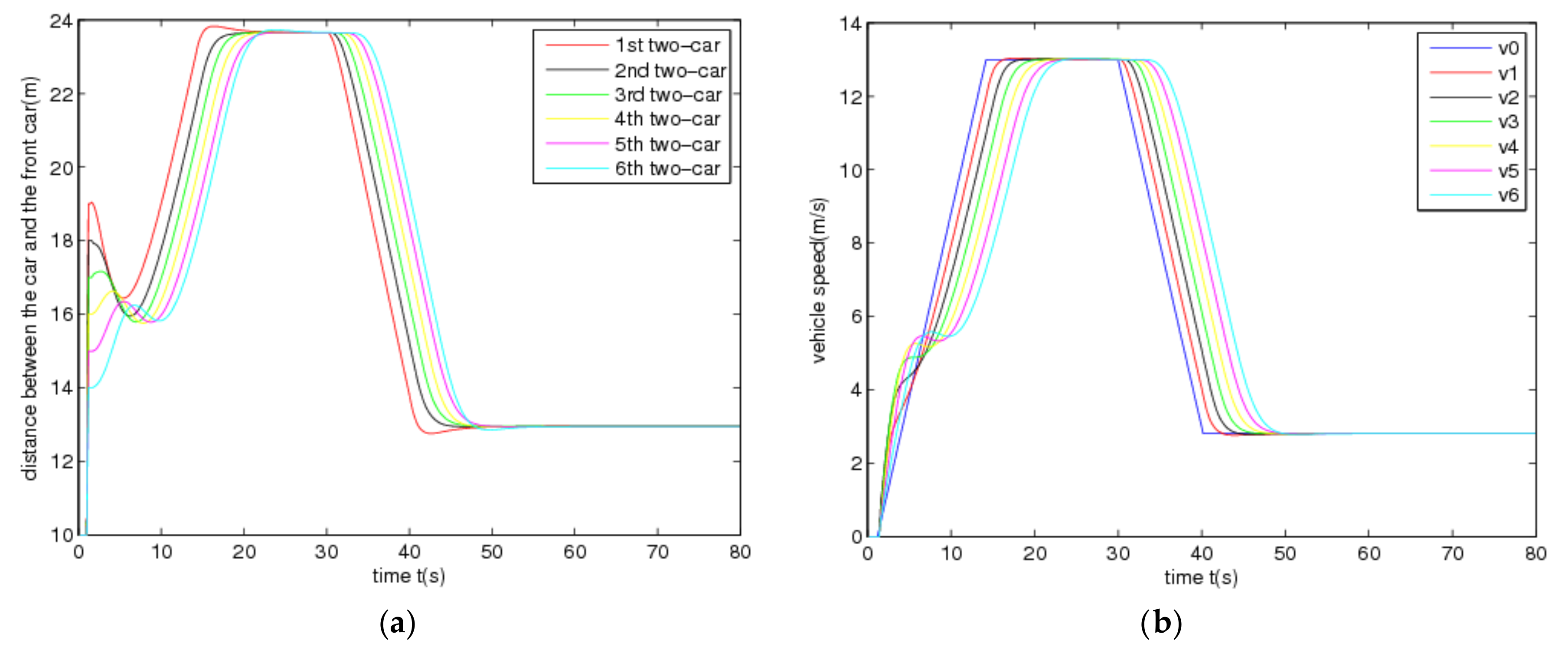
In the simulation study, the initial spacing errors e_i(0) of the vehicle platoon are set as e₁(0) = 9 m, e₂(0) = 8 m, e₃(0) = 7 m, e₄(0) = 6 m, e₅(0) = 5 m and e₆(0) = 4 m, and all cars of the vehicle platoon stop at initial time t=0. To begin with, the leading vehicle accelerates at 1 m/s² from 1 to 13 s and then cruises at the constant speed 13 m/s for lasting 8 secs. At time 31 s, due to the emerging traffic scenarios, e.g., front jamming, cars suddenly cutting-in from adjacent lanes, etc., the leading vehicle decelerates fast until the velocity gets to 2.9 m/s at the time 41 s and then cruises at the low speed. These driving behaviors are very common in real traffic scenarios, especially in urban environments. Under these traffic scenarios, Figure 2 shows the time evolutions of all vehicles controlled by the designed CACC controllers with the gains in Table 1, where the subplot (a) pictures the actual inter-vehicle distance (spacing) profiles between the adjacent vehicles and the subplots (b)–(d) picture the time evolutions of the vehicle velocity, acceleration and computed control signals of the host vehicles, respectively. Note that in simulation, the varying time-delay of the communication network is produced by a stochastic signal satisfying the range of [0, h] with h = 1.0 s.

From Figure 2, it is observed that the trajectories of all vehicles can quickly converge in the face of the uncertainties and varying time-delay induced by the communication transmission. In other words, each car has the ability to track its immediately preceding one and maintain the inter-vehicle distance at the desired safety spacing as well as ensuring common speeds of all cars for the vehicle platoon subject to uncertainties and varying delay under the varying speed traffic scenario. This suggests that the vehicle platoon with the designed CACC controllers is robust stable in the presence of the uncertainties and varying communication delay. Note that at the starting, each following vehicle has a fast, transient behavior of acceleration and control input in order to quickly response the behaviors of the leading vehicle. Due to different uncertainties, varying time-delay and initial state of each vehicle, the transient behaviors of all vehicle are different accordingly. 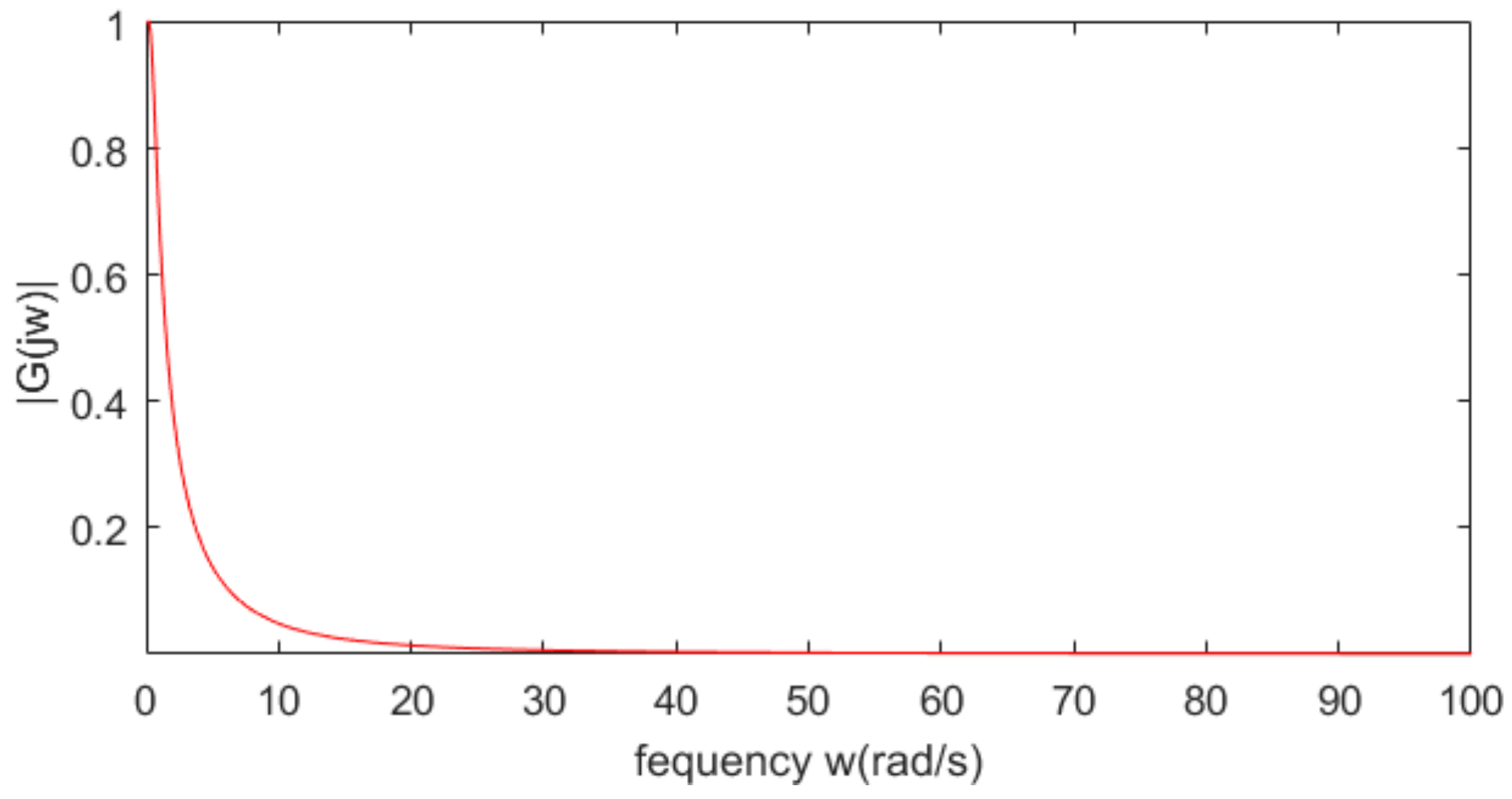Moreover, Figure 3 shows that the frequency response of the acceleration transfer function, G_i(jw), on the adjacent vehicles in the vehicle platoon with the CACC system. From Figure 3, it is observed that the frequency response of G_i(jw) satisfies that ‖G_i(jw)‖ ≤ 1 for any w ≥ 0, i = 1,…,6 in the presence of the uncertainties and varying communication delay. As a result, it is known from Definition 2 and Figure 2 and Figure 3 that the vehicle platoon with the CACC system has robust string stability for the uncertainties and varying time-delay of range [0, h]. This implies that the vehicle platoon with the designed CACC controllers has ability to attenuate spacing errors and velocity fluctuations resulted from the cars in front even in the presence of the uncertainties and varying communication delay. The robust stability and robust string stability performances of the CACC system are beneficial to improve and keep smooth traffic flow of roads. These results illustrate the effectiveness of the proposed robust CACC method for vehicle platoons subject to uncertainties and varying communication delay.

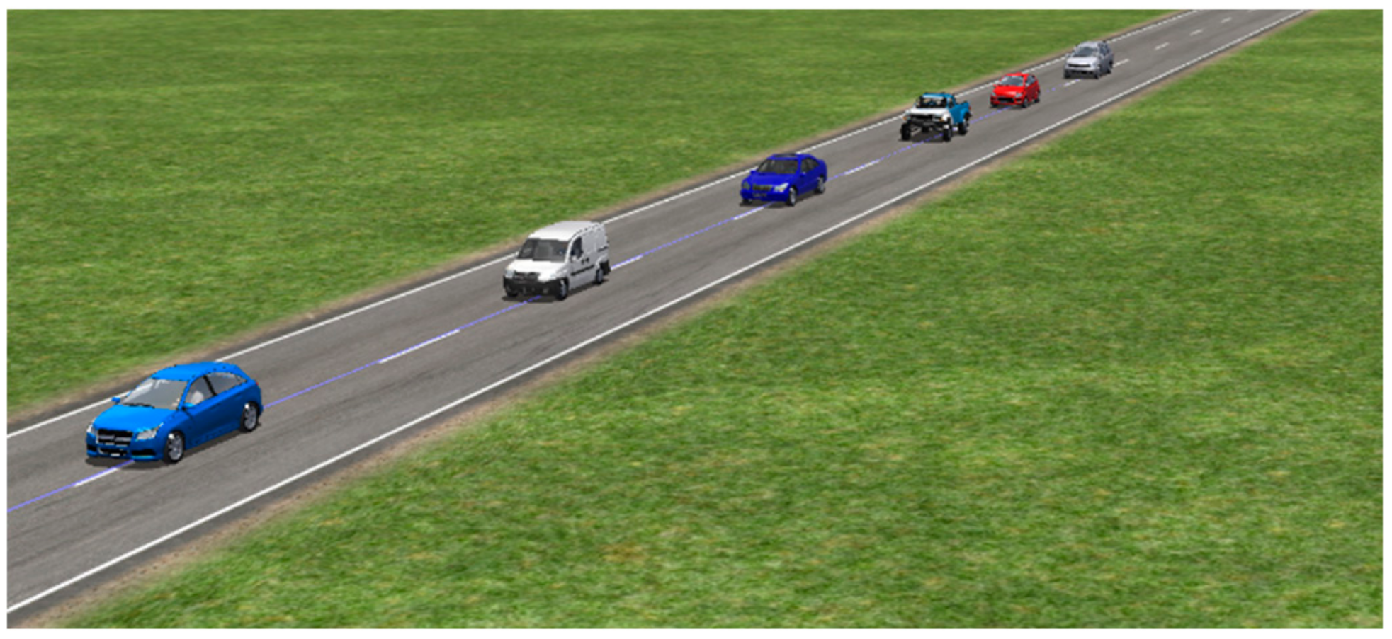
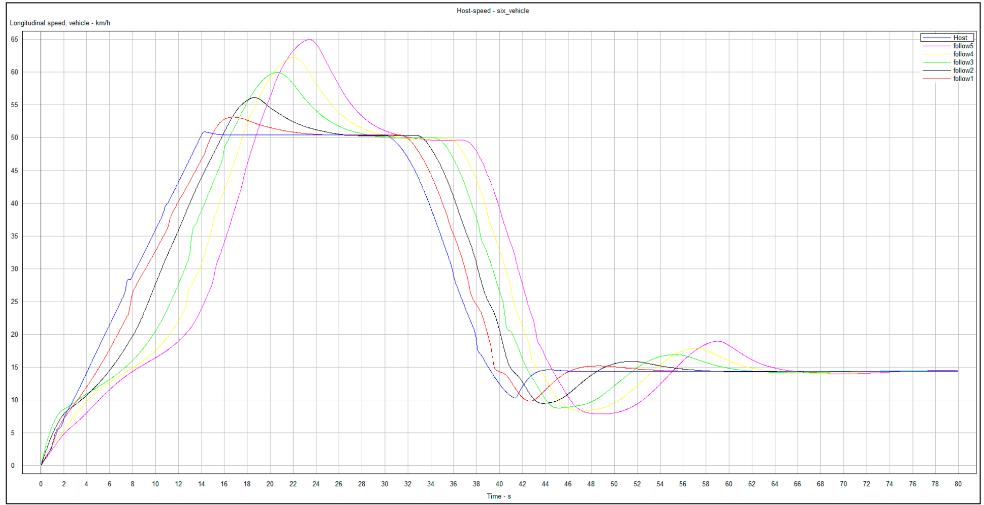
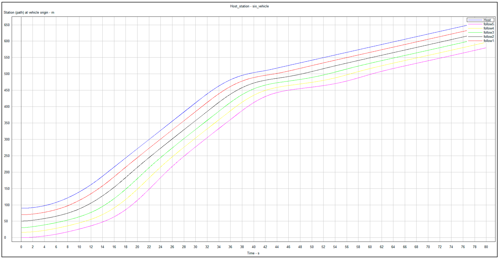
In order to further demonstrate the effectiveness of the presented CACC method, we use the CarSim2016.1 software to evaluate the stability performance of the control method. The software is a high-fidelity simulation environment with an interface for MATLAB/Simulink. In this experiment, six heterogeneous vehicles are used to make up a vehicle platoon which is shown in Figure 4. The vehicle types of the six vehicles are selected as C-Class Hatchback, European Van, F-Class Sedan, Off-Road Pickup, B-Class Hatchback, and D-Class Minivan, respectively. These different cars will be used to illustrate the applicability of the proposed CACC method to heterogeneous vehicle platoon. The velocity and acceleration of the leading car and simulation parameters are selected to be the same as the aforementioned MATLAB numerical experiment. The remaining parameters of these vehicles, e.g., the mass, transmission system and other parameters are selected to be the default values of the software.

In this co-simulation experiment of CarSim and Simulink, the CarSim software outputs the position, velocity and acceleration of each vehicle to Simulink at each time. Then, with the default parameters of the vehicular powertrain system and braking system, the throttle opening, or the main cylinder pressure output of each vehicle is computed by the input of CarSim and the controller in Simulink. The readers refer [34] for detailed co-simulation setup of CarSim and Simulink. Figure 5 and Figure 6 show the time profiles of velocity and position of the six vehicles, respectively. From Figure 5 and Figure 6, it can be seen that the vehicle platoon with the designed CACC controllers is robust stable and robust string stable in the presence of the uncertainties and varying time-delay. These results are the similar to those of the aforesaid MatLab simulation experiment, which further verify the robustness performance of the proposed CACC approach for vehicle platoons subject to uncertainties and varying communication delay.

From the aforesaid simulation results and discussions, it is known that the robust time-delay feedback CACC method is an effective strategy employed to achieve the goal of CACC for the vehicle platoon systems subject to uncertainties and varying communication delay. Therefore, these simulation results demonstrate the robust stability and robust string stability performances of the robust CACC method proposed in this paper.

6. Conclusions

In this paper, we presented a new robust cooperative adaptive cruise control method for vehicle platoons subject to parametric uncertainties and varying communication delay. A set of robust delay feedback CACC controllers was designed for the uncertain vehicle platoon with varying communication delay and was computed by solving some linear matrix inequalities. Moreover, the LMI conditions were established to guarantee the robust stability and robust string stability properties of the vehicle platoon in the presence of the uncertainties and varying time-delay. The results of simulation experiments demonstrated the effectiveness of the robust CACC method presented in this paper and evaluated the robust stability and robust string stability properties of the vehicle platoon subject to uncertainties and varying communication delay.

Since there generally exist nonlinearities and uncertainties in real vehicles, some interesting directions of future work include the investigation on nonlinear CACC methods and robust (string) stability of nonlinear vehicle platoons subject to varying time-delay induced by heterogeneous communication and vehicles’ actuators.

References

1. Silva, C.M.; Masini, B.M.; Ferrari, G.; Thibault, I. A survey on infrastructure-based vehicular networks. Mob. Inf. Syst. 2017, 2017, 1–28. [Google Scholar] [CrossRef] [Green Version]
2. Dey, K.C.; Yan, L.; Wang, X.; Wang, Y.; Shen, H.; Chowdhury, M.; Yu, L.; Qiu, C.; Soundararaj, V. A review of communication, driver characteristics, and controls aspects of cooperative adaptive cruise control (CACC). IEEE Trans. Intell. Transp. Syst. 2016, 17, 491–509. [Google Scholar] [CrossRef]
3. Wang, Z.; Wu, G.; Barth, M.J. A review on cooperative adaptive cruise control (CACC) systems: Achitectures, controls, and applications. In Proceedings of the 21st International Conference on Intelligent Transportation Systems (ITSC), Maui, HI, USA, 4–7 November 2018. [Google Scholar] [CrossRef] [Green Version]
4. Milanés, V.; Shladover, S.E.; Spring, J.; Nowakowski, C.; Kawazoe, H.; Nakamura, M. Cooperative adaptive cruise control in real traffic situations. IEEE Trans. Intell. Transp. Syst. 2014, 15, 296–305. [Google Scholar] [CrossRef] [Green Version]
5. Al-Jhayyish, A.M.H.; Schmidt, K.W. Feedforward strategies for cooperative adaptive cruise control in heterogeneous vehicle strings. IEEE Trans. Intell. Transp. Syst. 2018, 19, 113–122. [Google Scholar] [CrossRef]
6. Li, F.; Wang, Y. Cooperative adaptive cruise control for string stable mixed traffic: Benchmark and human-centered design. IEEE Trans. Intell. Transp. Syst. 2017, 18, 3473–3485. [Google Scholar] [CrossRef]
7. Guo, G.; Wang, Q. Fuel-efficient en route speed planning and tracking control of truck platoons. IEEE Trans. Intell. Transp. Syst. 2019, 20, 3091–3103. [Google Scholar] [CrossRef]
8. Van Nunen, E.; Reinders, J.; Semsar-Kazerooni, E.; van de Wouw, N. String stable model predictive cooperative adaptive cruise control for heterogeneous platoons. IEEE Trans. Intell. Veh. 2019, 4, 186–196. [Google Scholar] [CrossRef]
9. He, D.; Peng, B. Gaussian learning-based fuzzy predictive cruise control for improving safety and economy of connected vehicles. IET Intell. Transp. Syst. 2020, in press. [Google Scholar] [CrossRef]
10. Ploeg, J.; Van De Wouw, N.; Nijmeijer, H. Lp string stability of cascaded systems: Application to vehicle platooning. IEEE Trans. Control Syst. Technol. 2014, 22, 786–793. [Google Scholar] [CrossRef] [Green Version]
11. Feng, S.; Zhang, Y.; Li, S.E.; Cao, Z.; Liu, H.X.; Li, L. String stability for vehicular platoon control: Definitions and analysis methods. Annu. Rev. Control 2019, 47, 81–97. [Google Scholar] [CrossRef]
12. He, D.; Shi, Y.; Li, H.; Du, H. Multi-objective predictive cruise control for connected vehicle systems on urban conditions with InPA-SQP algorithm. Optim. Control Appl. Methods 2019, 40, 479–498. [Google Scholar] [CrossRef]
13. Wang, M.; Daamen, W.; Hoogendoorn, S.P.; Arem, B. Rolling horizon control framework for driver assistance systems-Part II: Cooperative sensing and cooperative control. Transp. Res. Part C 2014, 40, 290–311. [Google Scholar] [CrossRef]
14. He, D.; Qiu, T.; Luo, R. Fuel efficiency-oriented platooning control of connected nonlinear vehicles: A distributed economic MPC approach. Asian J. Control 2019, 21, 1–11. [Google Scholar] [CrossRef]
15. Kayacan, E. Multiobjective H control for string stability of cooperative adaptive cruise control systems. IEEE Trans. Intell. Veh. 2017, 2, 52–61. [Google Scholar] [CrossRef]
16. Li, Y.; Xu, C.; Xing, L.; Wang, W. Integrated cooperative adaptive cruise and variable speed limit controls for reducing rear-end collision risks near freeway bottlenecks based on micro-simulations. IEEE Trans. Intell. Transp. Syst. 2017, 18, 3157–3167. [Google Scholar] [CrossRef]
17. Guo, G.; Yue, W. Autonomous platoon control allowing range-limited sensors. IEEE Trans. Veh. Technol. 2012, 61, 2901–2912. [Google Scholar] [CrossRef]
18. Yu, S.; Wu, S.; Zhao, Y.; He, D. Delayed feedback MPC algorithm of vehicle platoons subject to constraints on measurement range and driving behaviors. Asian J. Control 2018, 20, 2260–2270. [Google Scholar] [CrossRef]
19. Oncu, S.; Ploeg, J.; van de Wouw, N.; Nijmeijer, H. Cooperative adaptive cruise control: Network-aware analysis of string stability. IEEE Trans. Intell. Transp. Syst. 2014, 15, 1527–1537. [Google Scholar] [CrossRef] [Green Version]
20. Firooznia, A.; Ploeg, J.; van de Wouw, N.; Zwart, H. Co-design of controller and communication topology for vehicular platooning. IEEE Trans. Intell. Transp. Syst. 2017, 18, 2728–2739. [Google Scholar] [CrossRef]
21. Orosz, G. Connected cruise control: Modelling, delay effects, and nonlinear behavior. Veh. Syst. Dyn. 2016, 54, 1147–1176. [Google Scholar] [CrossRef]
22. Abdessameuda, A.; Polushin, I.G.; Tayebi, A. Synchronization of nonlinear systems with communication delays and intermittent information exchange. Automatica 2015, 59, 1–8. [Google Scholar] [CrossRef]
23. Izadi, H.A.; Gordon, B.W.; Zhang, Y. Decentralized receding horizon control for cooperative multiple vehicles subject to communication delay. J. Guid. Control Dyn. 2009, 32, 1959–1965. [Google Scholar] [CrossRef]
24. Bernardo, M.; Salvi, A.; Santini, S. Distributed consensus strategy for platooning of vehicles in the presence of time-varying heterogeneous communication delays. IEEE Trans. Intell. Transp. Syst. 2015, 16, 102–112. [Google Scholar] [CrossRef]
25. Song, X.; Lou, X.; Meng, L. Time-delay feedback CACC of connected vehicles by heterogeneous channel trans-mission. Meas. Control 2019, 52, 369–378. [Google Scholar] [CrossRef] [Green Version]
26. Smith, O.J. A controller to overcome dead time. ISA Trans. 1959, 6, 28–33. [Google Scholar]
27. Shaqarin, T.; Al-Rawajfeh, A.E.; Hajaya, M.G.; Alshabatat, N.; Noack, B.R. Model-based robust H control of a granulation process using Smith predictor with reference updating. J. Process Control 2019, 77, 38–47. [Google Scholar] [CrossRef]
28. Zhu, Y.; Zhao, D.; Zhong, Z. Adaptive optimal control of heterogeneous CACC system with uncertain dynamics. IEEE Trans. Control Syst. Technol. 2019, 27, 1772–1779. [Google Scholar] [CrossRef]
29. Verginis, C.K.; Bechlioulis, C.P.; Dimarogonas, D.V.; Kyriakopoulos, K.J. Robust distributed control protocols for large vehicular platoons with prescribed transient and steady-state performance. IEEE Trans. Control Syst. Technol. 2018, 26, 299–304. [Google Scholar] [CrossRef] [Green Version]
30. Gao, F.; Li, S.; Zheng, Y.; Kum, D. Robust control of heterogeneous vehicular platoon with uncertain dynamics and communication delay. IET Intell. Transp. Syst. 2016, 10, 503–513. [Google Scholar] [CrossRef] [Green Version]
31. Zhang, X.M.; Wu, M.; She, J.; He, Y. Delay-dependent stabilization of linear systems with time-varying state and input delays. Automatica 2005, 41, 1405–1412. [Google Scholar] [CrossRef]
32. Boyd, S.; Ghaoui, L.E.; Feron, E.; Balakrishnan, V. Linear Matrix Inequalities in System and Control Theory; SIAM: Philadelphia, PA, USA, 1994. [Google Scholar]
33. He, D.; Huang, H.; Chen, Q. Quasi-min-max MPC for constrained nonlinear systems with guaranteed input-to-state stability. J. Frankl. Inst. 2014, 351, 3405–3423. [Google Scholar] [CrossRef]
34. Li, Y.; Deng, H.; Xu, X.; Wang, W. Modeling and testing of in-wheel motor drive intelligent electric vehicles based on co-simulation with Carsim/Simulink. IET Intell. Transp. Syst. 2019, 13, 115–123. [Google Scholar] [CrossRef]
Figure 1. A schematic CACC system of the vehicle platoon.
Sensors 20 01775 g001
Figure 2. Time evolutions of states and control of the vehicle platoon: (a) Actual spacing, (b) Velocity, (c) Acceleration, (d) Control signal.
Sensors 20 01775 g002aSensors 20 01775 g002b
Figure 3. Frequency response for any w ≥ 0.
Sensors 20 01775 g003
Figure 4. The six-vehicle platoon with CACC in CarSim.
Sensors 20 01775 g004
Figure 5. Velocity profiles of the six vehicles.
Sensors 20 01775 g005
Figure 6. Position profiles of the six vehicles.
Sensors 20 01775 g006