mGEODAR—A Mobile Radar System for Detection and Monitoring of Gravitational Mass-Movements

 , , , and
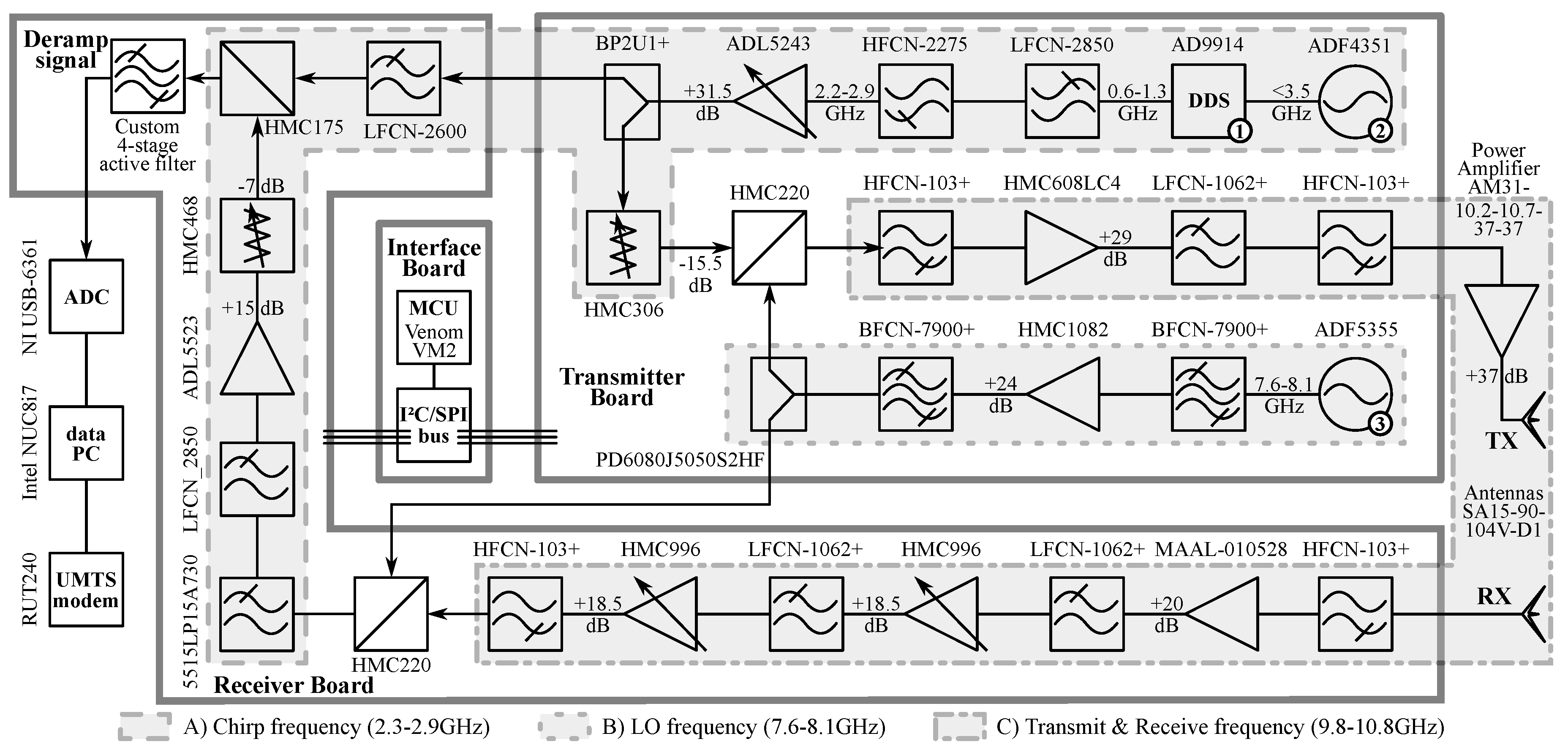
Abstract
:1. Introduction
2. Materials and Methods
2.1. Radar Hardware
2.2. FMCW Design Variables
2.3. Reconfigurable Signal Generation
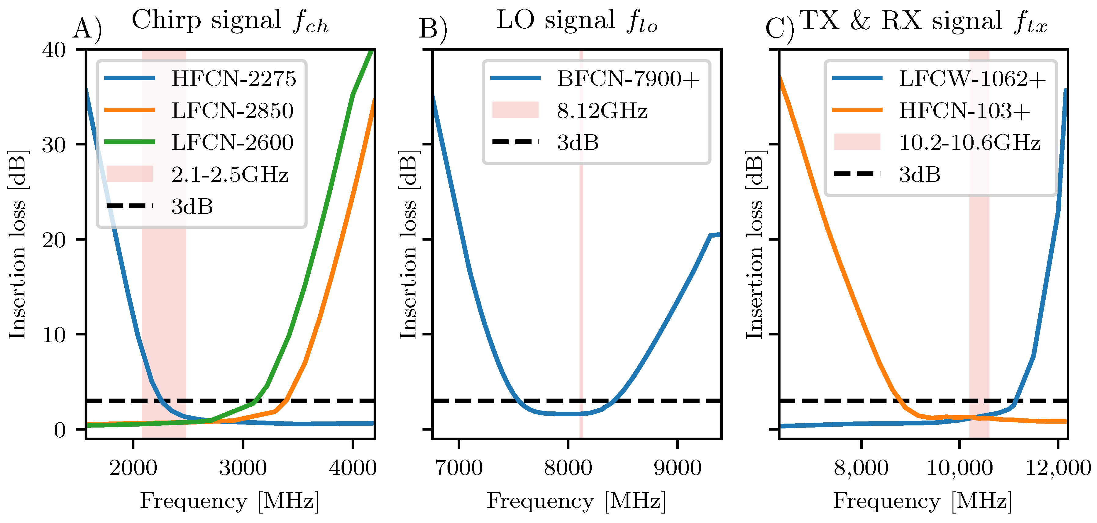
2.4. Baseband Filter
2.5. Digital Signal Processing
3. Measurements and Results
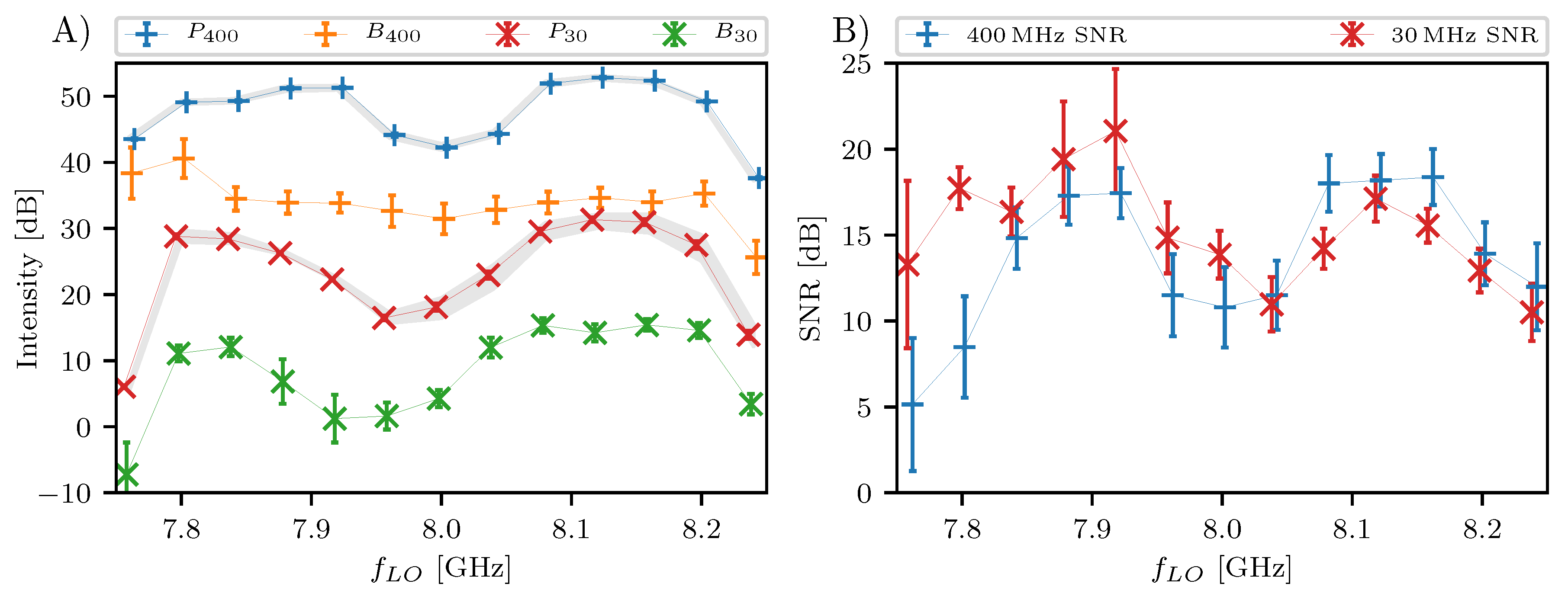
3.1. Signal Strength Optimization
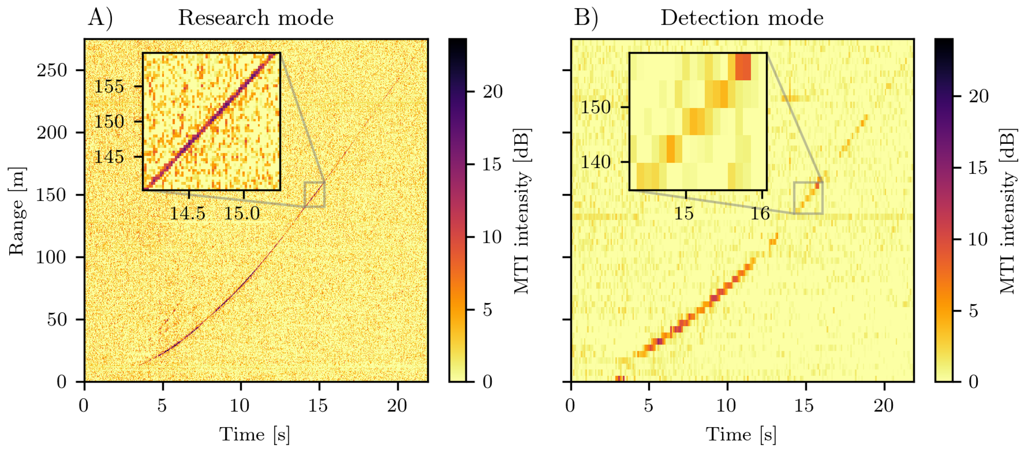
3.2. Moving Point Target
4. Discussion
5. Conclusions
Author Contributions
Funding
Acknowledgments
Conflicts of Interest
References
- Salm, B.; Gubler, H. Measurement and Analysis of the Motion of Dense Flow Avalanches. Ann. Glaciol. 1985, 6, 26–34. [Google Scholar] [CrossRef] [Green Version]
- Gauer, P.; Kern, M.; Kristensen, K.; Lied, K.; Rammer, L.; Schreiber, H. On pulsed Doppler radar measurements of avalanches and their implication to avalanche dynamics. Cold Reg. Sci. Tech. 2007, 6, 55–71. [Google Scholar] [CrossRef]
- Ash, M.; Brennan, P.V.; Chetty, K.; McElwaine, J.N.; Keylock, C.J. FMCW Radar Imaging of Avalanche-like Snow Movements. In Proceedings of the 2010 IEEE Radar Conference, Washington, DC, USA, 10–14 May 2010; pp. 102–107. [Google Scholar] [CrossRef]
- Vriend, N.M.; McElwaine, J.N.; Sovilla, B.; Keylock, C.J.; Ash, M.; Brennan, P.V. High-resolution Radar Measurements of Snow Avalanches. Geophys. Res. Lett. 2013, 40, 727–731. [Google Scholar] [CrossRef] [Green Version]
- Köhler, A.; McElwaine, J.N.; Sovilla, B.; Ash, M.; Brennan, P.V. The dynamics of surges in the 3 February 2015 avalanches in Vallée de la Sionne. J. Geophys. Res. 2016, 121, 2192–2210. [Google Scholar] [CrossRef] [Green Version]
- Faug, T.; Turnbull, B.; Gauer, P. Looking Beyond the Powder/Dense Flow Avalanche Dichotomy. J. Geophys. Res. 2018, 123, 1183–1186. [Google Scholar] [CrossRef]
- Köhler, A.; Sovilla, B.; McElwaine, J.N. 7 years of avalanche measurements with the GEODAR radar system. In Proceedings of the International Snow Science Workshop, Innsbruck, Austria, 7–12 October 2018; pp. 665–669. [Google Scholar]
- Ash, M.; Tanha, M.A.; Brennan, P.V.; Köhler, A.; McElwaine, J.N.; Keylock, C.J. Improving the sensitivity and phased array response of FMCW radar for imaging avalanches. In Proceedings of the 2014 International Radar Conference, Lille, France, 13–17 October 2014; pp. 1–5. [Google Scholar] [CrossRef]
- Ash, M.; Brennan, P.V.; Keylock, C.J.; Vriend, N.M.; McElwaine, J.N.; Sovilla, B. Two-Dimensional Radar Imaging of Flowing Avalanches. Cold Reg. Sci. Tech. 2014, 102, 41–51. [Google Scholar] [CrossRef] [Green Version]
- Peters, N.J.; Oppenheimer, C.; Brennan, P.; Lok, L.B.; Ash, M.; Kyle, P. Radar Altimetry as a Robust Tool for Monitoring the Active Lava Lake at Erebus Volcano, Antarctica. Geophys. Res. Lett. 2018, 45, 8897–8904. [Google Scholar] [CrossRef] [Green Version]
- Gentile, K. Super-Nyquist Operation of the AD9912 Yields a High RF Output Signal. Available online: http://www.analog.com/media/en/technical-documentation/application-notes/AN-939.pdf (accessed on 30 May 2020).
- Brennan, P.V.; Huang, Y.; Ash, M.; Chetty, K. Determination of Sweep Linearity Requirements in FMCW Radar Systems Based on Simple Voltage-Controlled Oscillator Sources. IEEE Trans. Aerosp. Electron. Syst. 2011, 47, 1594–1604. [Google Scholar] [CrossRef]
- Ash, M.; Brennan, P.V. Transmitter noise considerations in super-Nyquist FMCW radar design. IEEE Electron. Lett. 2015, 51, 413–415. [Google Scholar] [CrossRef] [Green Version]
- Federal Ministry for Transport, Innovation and Technology (BMVIT). Frequenznutzungsverordnung 2013, BGBl. II Nr. 63/2014 (German). Available online: https://www.ris.bka.gv.at/eli/bgbl/II/2014/63/20140324 (accessed on 14 September 2020).
- Stove, A.G. Modern FMCW radar—Techniques and applications. In Proceedings of the First European Radar Conference, Amsterdam, The Netherlands, 11–15 October 2004; pp. 149–152. [Google Scholar]
- Köhler, A. High Resolution Radar Imaging of Snow Avalanches. Ph.D. Thesis, Durham University, Durham, UK, 2018. [Google Scholar]
- Köhler, A.; McElwaine, J.N.; Sovilla, B. GEODAR Data and the Flow Regimes of Snow Avalanches. J. Geophys. Res. 2018, 123, 1272–1294. [Google Scholar] [CrossRef]
- Taraldsen, G.; Berge, T.; Haukland, F.; Lindqvist, B.H.; Jonasson, H. Uncertainty of decibel levels. J. Acoust. 2015, 138, EL264–EL269. [Google Scholar] [CrossRef] [Green Version]
- Ash, M. FMCW Phased Array Radar for Imaging Snow Avalanches. Ph.D. Thesis, University College London, London, UK, 2013. [Google Scholar]
- Long, D.A.; Reschovsky, B.J. Electro-optic frequency combs generated via direct digital synthesis applied to sub-Doppler spectroscopy. OSA Continuum. 2019, 2, 3576–3583. [Google Scholar] [CrossRef]


Publisher’s Note: MDPI stays neutral with regard to jurisdictional claims in published maps and institutional affiliations. |
© 2020 by the authors. Licensee MDPI, Basel, Switzerland. This article is an open access article distributed under the terms and conditions of the Creative Commons Attribution (CC BY) license (http://creativecommons.org/licenses/by/4.0/).
Share and Cite
Köhler, A.; Lok, L.B.; Felbermayr, S.; Peters, N.; Brennan, P.V.; Fischer, J.-T. mGEODAR—A Mobile Radar System for Detection and Monitoring of Gravitational Mass-Movements. Sensors 2020, 20, 6373. https://doi.org/10.3390/s20216373
Köhler A, Lok LB, Felbermayr S, Peters N, Brennan PV, Fischer J-T. mGEODAR—A Mobile Radar System for Detection and Monitoring of Gravitational Mass-Movements. Sensors. 2020; 20(21):6373. https://doi.org/10.3390/s20216373
Chicago/Turabian StyleKöhler, Anselm, Lai Bun Lok, Simon Felbermayr, Nial Peters, Paul V. Brennan, and Jan-Thomas Fischer. 2020. "mGEODAR—A Mobile Radar System for Detection and Monitoring of Gravitational Mass-Movements" Sensors 20, no. 21: 6373. https://doi.org/10.3390/s20216373
APA StyleKöhler, A., Lok, L. B., Felbermayr, S., Peters, N., Brennan, P. V., & Fischer, J.-T. (2020). mGEODAR—A Mobile Radar System for Detection and Monitoring of Gravitational Mass-Movements. Sensors, 20(21), 6373. https://doi.org/10.3390/s20216373