Abstract
Internet of Things (IoT) is characterized by a system of interconnected devices capable of communicating with each other to carry out specific useful tasks. The connection between these devices is ensured by routers distributed in a network. Optimizing the placement of these routers in a distributed wireless sensor network (WSN) in a smart building is a tedious task. Computer-Aided Design (CAD) programs and software can simplify this task since they provide a robust and efficient tool. At the same time, experienced engineers from different backgrounds must play a prominent role in the abovementioned task. Therefore, specialized companies rely on both; a useful CAD tool along with the experience and the flair of a sound expert/engineer to optimally place routers in a WSN. This paper aims to develop a new approach based on the interaction between an efficient CAD tool and an experienced engineer for the optimal placement of routers in smart buildings for IoT applications. The approach follows a step-by-step procedure to weave an optimal network infrastructure, having both automatic and designer-intervention modes. Several case studies have been investigated, and the obtained results show that the developed approach produces a synthesized network with full coverage and a reduced number of routers.
1. Introduction
With the advent of low-power high-fidelity sensors capable of making precise measurements of the environmental parameters, the need to effectively link them in a network has arisen. Wireless communication networks have successfully replaced wired connections for efficient data transmission between sensor nodes, via radio communication. As a result, wireless sensor networks (WSN) have come into existence, and are playing an essential role in our daily lives [1]. WSNs also play a pivotal role in realizing the recent development of the Internet of Things (IoT), where the applications of such networks include security systems, environment monitoring, healthcare systems, and smart homes to name a few [2]. In one of the recent IoT applications, a WSN connects the legacy electrical equipment, incapable of communicating with standard protocols, with the smart grid controller [3]. The concept receives further attention from the research community when it is incorporated in an entire building to monitor and control appliances so that the building is automated. The purpose of this automation can be to make the building energy-efficient, or environmentally and inhabitant friendly. These automation systems are known as the building automation system (BAS). Energy efficiency is not only a focal point of research for large systems but also for systems as small as the sensors themselves [4,5]. Moreover, researchers are seeking adaptive solutions capable of providing more stable network performance with optimal network paths and resources [6].
Designing WSNs for the BAS has been a challenging task for the research community. Usually, while establishing an optimal arrangement of a network system, conflicting objective functions might arise [7]. A joint optimization model has been developed in [8] to optimize power, rate, and delay of radio sensor networks collectively. In [9], a large scale WSN is considered where authors utilize the genetic algorithm to determine the moving trajectory of the mobile sinks and an improved version of particle swarm optimization (PSO) to ascertain parking positions so that coverage rate is optimized. The same group developed the PSO-based coverage control algorithm in [10] considering both coverage rate and ensuring reduced energy consumption. On a smaller scale, an indoor localization of routers has been carried out in [11] using an interpolation algorithm and dual-frequency bands. For enhancing data collection rata, [12] presents a data-aggregation-based algorithm formulated as a linear programming problem. Energy-efficient software-defined WSNs are proposed by combining content awareness and adaptive data broadcast in [13], increasing the sensor’s lifespan. In [14,15], the authors utilized a CAD tool to model, simulate, and automate code generation for the optimal placement of routers in the design of WSN for BAS. Its extension was presented in [16], where the authors developed an interactive tool for network synthesis. The improved version of that in [16] claims to reduce design time while improving the quality of network topology. They offer a crude simulation-based trial-and-error approach to simulate multiple topologies one by one and select the better performing solution without the guarantee of optimality. It provides a graphical user interface (GUI) where a designer places the routers in a 2D floor plan to establish the connection between end devices (EDs)—which include sensors and actuators—and the base station (BS). This GUI provides a router placement plan for a single floor, considering that this is how building floors are distributed in rented residential units and offices. An exciting alternative was proposed in [17], where the duct system of a building is used as a waveguide to establish communication between various WSNs. The optimal placement of the sensor is not limited to BAS only. For example, in [18], a preferred placement of sensors to monitor human activity using smart textile systems and inertial measurement units, was presented.
Similarly, in [19,20], a GUI based interactive tool was developed for optimal placement of router nodes while considering different propagation models and terrain obstacles depicted in the floor plan. Reference [19] presents two methods to design the architecture of the WSN backbone: mixed integer linear programming (MILP) and the Dijkstras algorithm. The former one gives the exact solution to the problem for a network consisting of about 50 nodes in an hour. In contrast, the second method gives the suboptimal solution but was significantly faster than the first method. MILP, a computationally expensive method, was also utilized in [21] to design a WSN. In [22], the neural-gas algorithm was utilized to design the BAS, where it takes the information of building geometry, target constraints, and special zones and comes up with the candidate solutions for placing sensors in the network. Reference [22] differs from [16] in the sense that it determined the optimal placement of sensors, whereas [16] gave the optimal solution for a routers’ location that connects EDs with BS.
Another similar approach is developed in [23]. However, instead of the neural-gas algorithm, it used simulated annealing. It deployed a method of partitioning in which target space is subdivided into smaller sub-regions to deal with the dynamic environment of each sub-region. In this work, however, the target space is not explicitly divided, and the algorithm will automatically take care of the spatial variations. Search oriented strategies, primarily based on simulated annealing, were presented in [24]. It also considers the radiation pattern of antennae while determining the sensor positions. The algorithm looks for those positions of the nodes in the search space that satisfy the connectivity and coverage constraints. Instead of a WSN, Reference [25] used simulated annealing to find the optimal location of mesh routers in a wireless mesh network. In this paper, the underlying optimization algorithm remains the same, but the network has an additional gateway router to be considered while deploying communication protocols. The same objective was achieved in [26] using the firefly optimization algorithm, instead of simulated annealing. Other coverage constraints are beyond the scope of this work, as it is focused on ensuring the connectivity of fixed EDs to the BS. Another grid-based nodes deployment technique was presented in [27,28], to maximize the coverage of network sensors; however, the problem turns out to be constrained, in terms of being truly optimal, due to limited search space.
The main contributions of this paper are:
- The development and deployment of a new technique that would result in a synthesis of backbone network architecture having a smaller number of routers in smaller amount of time, ensuring high fidelity connectivity between the EDs and the BS, throughout the target space.
- Develop an interactive CAD based on a smart approach for optimal router placement.
- Combine the benefits of the developed CAD and the experience of design engineers in an automatized manner.
2. Proposed Approach
2.1. Walkthrough
The proposed approach takes a step-by-step approach to develop the synthesized structure of routers. The flowchart of this approach is given in Figure 1. In the first step, the input data are provided by the user—the floor plan, the position of the BS, the Eds, and the thicknesses of the walls. Furthermore, communication parameters, like the operating frequency of the wireless sensors, are fed into the algorithm.
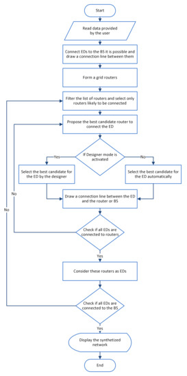
Figure 1.
Flowchart of the proposed approach.
The Free Space Path Loss (FSPL) in (dB) between two routers is given by:
where is the distance between the two routers [m], is the frequency [GHz], is the light speed [m/s], is the transmitter gain [dB] and is the receiver gain [dB].
In this paper, an operating frequency of 2.4 GHz is considered, and are supposed to be null, a −75 dB communication range (minimum FSPL) is assumed in a lossless free space medium. Equation (1) indicates that the assumed minimum FSPL is equivalent to 55 m as a maximal distance between two connected sensors (if there are no walls or obstacles in between). If there is an obstacle between the two sensors this 55 m distance is reduced in the function of the obstacle (or wall) thickness.
In the second step, a connection is established between the BS and EDs situated nearby. To be precise, EDs situated within a range of 55 m are linked to the BS, and a subsequent connection line—a thick black colored line—is then drawn to show that this ED has been connected. Later, in step 3, a grid of N × M potential routers is constructed over the entire floor plan. Routers placed on walls or obstacles are slightly moved to avoid the overlap.
In step 4, it was realized that not all routers can be connected to EDs. Therefore, the information of the routers that are likely to be connected to an ED (i.e., routers within 55 m range from EDs) are kept for the next step, and the remaining routers are removed, reducing the size of feed-forward matrices and consequently minimizing the processing time.
In the fifth step, the algorithm can either propose the best candidate router or automatically select the best candidate router for each ED, depending on the mode selected. The mechanism of selecting the best candidate router is the same as the one presented in [29]. In this mechanism, routers are sorted, and the ones with the ability to connect to more routers and are near to the BS are ranked highest. The first ranked router is the best candidate router. For example, if there are two routers where the first one can connect to two EDs while the second one can connect to three EDs, the second one is ranked better than the first one. This is the same if two routers have the same number of potential connections to EDs; however, if the first one is nearer to the BS then it is ranked better than the second one.
In the first mode of operation, the designer can either approve the algorithm proposal or select a different router based on his experience or any other external factor that the algorithm cannot take into consideration. A blue-colored connection line is drawn to show that this ED has been connected. This operation is repeated until all EDs are connected.
In step 6, the previously connected routers take the role of EDs, and the process from step 2 to step 5 is repeated until all EDs are fully connected to the BS via best candidate routers. In the end, the entire synthesized network is displayed.
2.2. Illustration with a Simple Network Setup
Step 1 deals with reading and storing all the data given by the user such as the dimensions of the layout, the obstacles, the EDs numbers and locations, and the BS location. In this illustrative example there are 19 EDs located at (50 m, 50 m), (150 m, 50 m), (150 m, 200 m), (400 m, 250 m), (450 m, 200 m), (50 m, 350 m), (100 m, 350 m), (200 m, 350 m), (450 m, 350 m), (450 m, 300 m), (300 m, 100 m), (350 m, 75 m), (150 m, 150 m), (350 m, 100 m), (300 m, 350 m), (50 m, 300 m), (125 m, 175 m), (450 m, 50 m), (450 m, 100 m) and (250 m, 240 m) and one BS located at (250 m, 200 m). The initial layout has a dimension of (500 m × 400 m), as shown in Figure 2a where EDs are represented by cyan colored circles whilst the BS is represented by a green-colored square. The origin (0 m, 0 m) is located in the upper left corner of the layout. Step 2 connects the EDs to the BS if they lie in close vicinity. In this example, there is one ED that can be connected directly to the BS because the distance between them is less than 55 m, as shown in Figure 2b. Consequently, in step 3, a grid of 24 × 30 = 720 potential routers is constructed over the entire floor plan, as shown in Figure 2c. Step 4 keeps only those routers that are likely to be connected to an ED and discards remaining routers from the list of potential routers, as shown in Figure 2d.
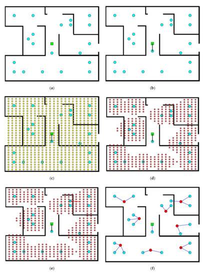
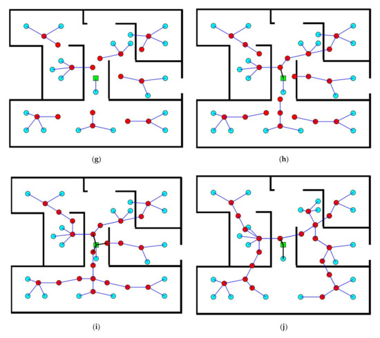
Figure 2.
Illustrative example: (a) Initial layout; (b) Connection of an end device (ED) to the base station (BS); (c) grid construction over the entire floor plan; (d) routers list filtering; (e) best router proposal for a given ED; (f) connection of all EDs to routers; (g) connection of the first set of routers to a second set; (h) connection of the second set of routers to a third set; (i) final design; and (j) an alternative final design.
Assuming the selection of designer mode for step 5 of this illustration, the algorithm proposes the best candidate router to connect to each ED one by one. This choice is represented by a thick red line, as shown in Figure 2e. Whether the designer approves this choice or not, the whole process is repeated until all EDs are connected, as shown in Figure 2f where red circles represent connected routers.
Step 6 considers previously connected routers as EDs and the process from step 2 to step 5 is repeated until all the initial EDs are connected to the BS as shown in Figure 2g,h. Once all EDs are connected to the BS, the optimal network is obtained, as shown in Figure 2i. Based on designer choices, other networks can also be obtained. An alternative network choice is shown in Figure 2j. The first obtained design is composed of 22 routers, whilst the second one is composed of 21 routers.
3. Application and Results
The developed approach has been tested on different floor plans using a variety of dimensions and sizes and different numbers of EDs. The obtained networks have been compared with the synthesized networks using the CAD tool developed in [29].
3.1. Case Study 1
The initial layout (430 m × 420 m) for this case is given in Figure 3a. There are 13 EDs and 1 BS. The synthesized network using the fully automatized CAD tool is given in Figure 3b while the one obtained using the proposed approach is given in Figure 3c. It can be seen from these figures that, for the first network, there are 18 placed routers whilst for the second network, there are 16 placed routers. It can also be noticed that the synthesized network using the proposed approach is much more optimized than the one using the CAD tool without the interaction of the expert designer.
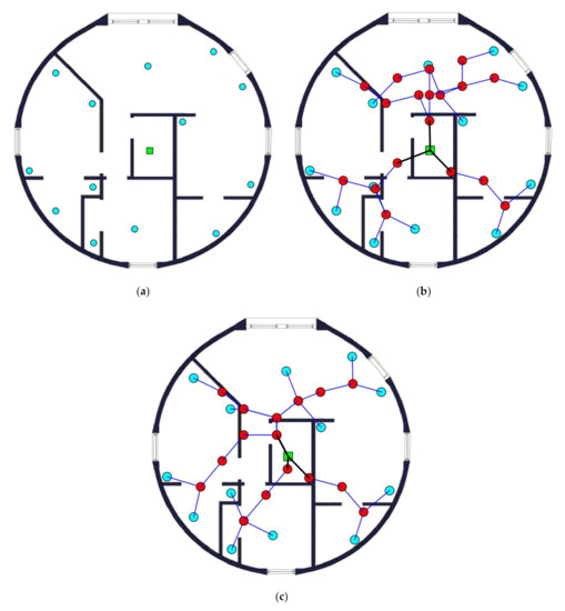
Figure 3.
Case study 1: (a) Initial layout; (b) synthesized network using the CAD tool; and (c) synthesized network using the proposed approach.
The detailed information about the synthesized network is tabulated in Table 1. In this table, the first column represents the node BS, ED or router number, the second column shown the type of the node where ‘1’ stands for BS node, ‘2’ stands for ED, ‘3’ stands for the router, and the last two columns represent the x-coordinate and y-coordinate of each node, respectively.

Table 1.
Nodes of the synthesized network using the proposed approach for case study 1.
3.2. Case Study 2
For this case study, the initial layout has the dimensions of (310 m × 270 m), as shown in Figure 4a. The area is equipped with 15 EDs and 1 BS. Figure 4b shows the synthesized network obtained using a fully automatized CAD tool, while Figure 4c displays the one obtained using the proposed approach. With a fully automized CAD tool, 16 routers are placed, whereas the proposed algorithm offers the solution by optimally placing only 14 routers. In congruence with the previous case study, the synthesized network using the proposed approach produces better results than those using the CAD tool only. The detailed information about the synthesized network obtained using the proposed approach is tabulated in Table 2.
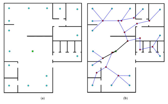
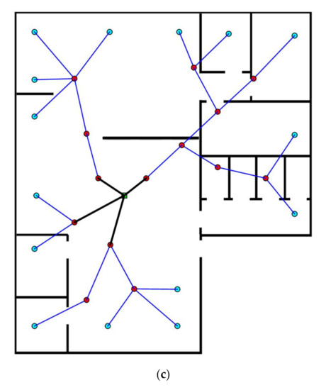
Figure 4.
Case study 2: (a) Initial layout; (b) synthesized network using the CAD tool; and (c) synthesized network using the proposed approach.
Table 2.
Nodes of the synthesized network using the proposed approach for case study 2.
3.3. Case Study 3
In case three, the layout dimensions are (380 m × 340 m), the number of EDs are 40 with 1 BS, as shown in Figure 5a. Without expert intervention, i.e., only using the CAD, the network architecture obtained is shown in Figure 5b, whereas, the one obtained using the proposed approach is depicted in Figure 5c. The proposed technique provides the solution with 19 routers in comparison with 30 routers which were obtained using the CAD only approach. Thus, an optimal result is obtained using the proposed approach. Table 3 tabulates the necessary information related to the coordinates and the position of every node in the network.
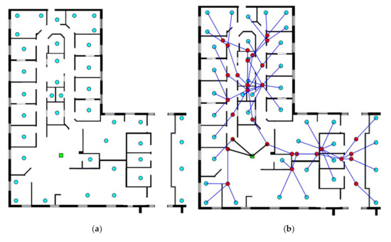
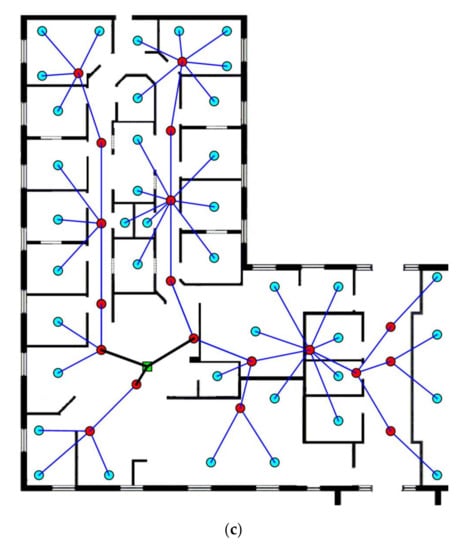
Figure 5.
Case study 3: (a) Initial layout; (b) synthesized network using the CAD tool; and (c) synthesized network using the proposed approach.
Table 3.
Nodes of the synthesized network using the proposed approach for case study 3.
4. Conclusions
In this paper, a new efficient and interactive synthesis algorithm for optimal router placement in WSNs has been proposed, developed, and implemented. This algorithm has been first illustrated using a simple network setup. Then, three case studies, with different difficulties and configurations, were investigated to test the validity of the proposed algorithm. Finally, a case study at the University of Hafr Al Batin was investigated. The obtained results are satisfactory compared to the use of CAD only. The interaction between the designer and the CAD led to better results.
However, there are some perspectives to investigate in future studies. One aspect could be the design of WSNs with some redundancy to avoid network failure that can be caused by nodes failures. Another future axis could be to include more details about the building, such as the types of materials used for walls and windows. Finally, considering more than one base station could also be investigated in our future work.
Author Contributions
All authors discussed the results and contributed to the final manuscript. H.R.E.H.B. and M.S.J. developed the CAD tool and performed the numerical simulations. M.A.A. conceived the original idea and supervised the project. All authors have read and agreed to the published version of the manuscript.
Funding
This research was funded by the Deanship of Scientific Research, University of Hafr Al Batin, grant number G-101-2020.
Acknowledgments
The authors extend their appreciation to the Deanship of Scientific Research, University of Hafr Al Batin, for funding this work through the research group project No G-101-2020.
Conflicts of Interest
The authors declare no conflict of interest.
Abbreviations
| BS | Base Station |
| BAS | Building Automation System |
| CAD | Computer-Aided Design |
| EDs | End Devices |
| GUI | Graphical User Interface |
| IoT | Internet of Things |
| MILP | Mixed Integer Linear Programming |
| WSN | Wireless Sensor Network |
References
- Obeid, A.M.; Karray, F.; Jmal, M.W.; Abid, M.; Qasim, S.M.; BenSaleh, M.S. Towards realization of wireless sensor network-based water pipeline monitoring systems: A comprehensive review of techniques and platforms. IET Sci. Meas. Technol. 2016, 10, 420–426. [Google Scholar] [CrossRef]
- Serra, R.; Nabi, M. Wireless coexistence and interference test method for low-power wireless sensor networks. IET Sci. Meas. Technol. 2015, 9, 563–569. [Google Scholar] [CrossRef]
- De Araújo, P.; Filho, R.; Rodrigues, J.; Oliveira, J.; Braga, S. Infrastructure for Integration of Legacy Electrical Equipment into a Smart-Grid Using Wireless Sensor Networks. Sensors 2018, 18, 1312. [Google Scholar] [CrossRef] [PubMed]
- Tümer, A.E.; Gündüz, M. Energy-Efficient and Fast Data Gathering Protocols for Indoor Wireless Sensor Networks. Sensors 2010, 10, 8054–8069. [Google Scholar] [CrossRef] [PubMed]
- Cerchecci, M.; Luti, F.; Mecocci, A.; Parrino, S.; Peruzzi, G.; Pozzebon, A. A Low Power IoT Sensor Node Architecture for Waste Management Within Smart Cities Context. Sensors 2018, 18, 1282. [Google Scholar] [CrossRef] [PubMed]
- Jutila, M. An Adaptive Edge Router Enabling Internet of Things. IEEE Internet Things J. 2016, 3, 1061–1069. [Google Scholar] [CrossRef]
- Yu, W.; Li, X.; Yang, H.; Huang, B. A multi-objective metaheuristics study on solving constrained relay node deployment problem in WSNS. Intell. Autom. Soft Comput. 2018, 24, 367–376. [Google Scholar] [CrossRef]
- Ssajjabbi Muwonge, B.; Pei, T.; Sansa Otim, J.; Mayambala, F. A Joint Power, Delay and Rate Optimization Model for Secondary Users in Cognitive Radio Sensor Networks. Sensors 2020, 20, 4907. [Google Scholar] [CrossRef] [PubMed]
- Wang, J.; Gao, Y.; Zhou, C.; Simon Sherratt, R.; Wang, L. Optimal coverage multi-path scheduling scheme with multiple mobile sinks for WSNs. Comput. Mater. Contin. 2020, 62, 695–711. [Google Scholar] [CrossRef]
- Wang, J.; Ju, C.; Gao, Y.; Sangaiah, A.K.; Kim, G.J. A PSO based energy efficient coverage control algorithm for wireless sensor networks. Comput. Mater. Contin. 2018, 56, 433–446. [Google Scholar]
- Yang, J. Indoor Localization System Using Dual-Frequency Bands and Interpolation Algorithm. IEEE Internet Things J. 2020, 1. [Google Scholar] [CrossRef]
- Lin, H.; Bai, D.; Gao, D.; Liu, Y. Maximum Data Collection Rate Routing Protocol Based on Topology Control for Rechargeable Wireless Sensor Networks. Sensors 2016, 16, 1201. [Google Scholar] [CrossRef] [PubMed]
- Buzura, S.; Iancu, B.; Dadarlat, V.; Peculea, A.; Cebuc, E. Optimizations for Energy Efficiency in Software-Defined Wireless Sensor Networks. Sensors 2020, 20, 4779. [Google Scholar] [CrossRef] [PubMed]
- Mozumdar, M.M.R.; Gregoretti, F.; Lavagno, L.; Vanzago, L.; Olivieri, S. A framework for modeling, simulation and automatic code generation of sensor network applications. In Proceedings of the 5th Annual Communications Society Conference on Sensor, Mesh and Ad Hoc Communications and Networks, SECON’, San Francisco, CA, USA, 16–20 June 2008; pp. 515–522. [Google Scholar]
- Rahman Mozumdar, M.M.; Lavagno, L.; Vanzago, L.; Sangiovanni-Vincentelli, A.L. HILAC: A framework for Hardware in the Loop simulation and multi-platform automatic code generation of WSN applications. In Proceedings of the International Symposium on Industrial Embedded Systems (SIES), Trento, Italy, 7–9 July 2010; pp. 88–97. [Google Scholar]
- Mozumdar, M.M.R.; Ganesan, A.; Ameri, A. Synthesizing sensor networks backbone architecture for smart buildings. IEEE Sens. J. 2014, 14, 4273–4283. [Google Scholar] [CrossRef]
- Yang, H.; Kim, B.; Lee, J.; Ahn, Y.; Lee, C. Advanced Wireless Sensor Networks for Sustainable Buildings Using Building Ducts. Sustainability 2018, 10, 2628. [Google Scholar] [CrossRef]
- Mokhlespour Esfahani, M.; Nussbaum, M. Preferred Placement and Usability of a Smart Textile System vs. Inertial Measurement Units for Activity Monitoring. Sensors 2018, 18, 2501. [Google Scholar] [CrossRef] [PubMed]
- Puggelli, A.; Mozumdar, M.M.R.; Lavagno, L.; Sangiovanni-Vincentelli, A.L. Routing-aware design of indoor wireless sensor networks using an interactive tool. IEEE Syst. J. 2015, 9, 717–727. [Google Scholar] [CrossRef]
- Mozumdar, M.; Ganesan, A.; Daragheh, A.A. Optimizing router nodes placement for designing distributed sensor networks. In Proceedings of the 2014 International Conference on Distributed Computing in Sensor Systems (DCOSS 2014), Marina Del Rey, CA, USA, 26–28 May 2014; pp. 344–348. [Google Scholar]
- Pinto, A.; D’Angelo, M.; Fischione, C.; Scholte, E.; Sangiovanni-Vincentelli, A. Synthesis of embedded networks for building automation and control. In Proceedings of the American Control Conference, Seattle, WA, USA, 11–13 June 2008; pp. 920–925. [Google Scholar]
- McGibney, A.; Klepal, M.; O’Donnell, J.T. Design of underlying network infrastructure of smart buildings. In Proceedings of the 4th International Conference on Intelligent Environments, Seattle, WA, USA, 21–22 July 2008; pp. 1–4. [Google Scholar]
- Wang, Y.C.; Hu, C.C.; Tseng, Y.C. Efficient deployment algorithms for ensuring coverage and connectivity of wireless sensor networks. In Proceedings of the 1st International Conference on Wireless Internet (WICON 2005), Budapest, Hungary, 10–15 July 2005; pp. 114–121. [Google Scholar]
- Chang, J.J.; Hsiu, P.C.; Kuo, T.W. Search-oriented deployment strategies for wireless sensor networks. In Proceedings of the 10th International Symposium on Object and Component-Oriented Real-Time Distributed Computing (ISORC 2007), Thera, Greece, 7–9 May 2007; pp. 164–171. [Google Scholar]
- Sayad, L. Optimal placement of mesh routers in a wireless mesh network with mobile mesh clients using simulated annealing. In Proceedings of the 5th International Symposium on Computational and Business Intelligence(ISCBI 2017), Dubai, UAE, 11–14 August 2017; pp. 45–49. [Google Scholar]
- Sayad, L.; Aissani, D.; Bouallouche-Medjkoune, L. Placement optimization of wireless mesh routers using firefly optimization algorithm. In Proceedings of the 2018 International Conference on Smart Communications in Network Technologies (SaCoNeT 2018), El Oued, Algeria, 27–31 October 2018; pp. 144–148. [Google Scholar]
- Akshay, N.; Kumar, M.P.; Harish, B.; Dhanorkar, S. An efficient approach for sensor deployments in wireless sensor network. In Proceedings of the International Conference on Emerging Trends in Robotics and Communication Technologies (INTERACT 2010), Chennai, India, 3–5 December 2010; pp. 350–355. [Google Scholar]
- Bai, X.; Kumar, S.; Xuan, D.; Yun, Z.; Lai, T.H. Deploying wireless sensors to achieve both coverage and connectivity. In Proceedings of the International Symposium on Mobile Ad Hoc Networking and Computing (MobiHoc), Florence, Italy, 22–25 May 2006; pp. 131–142. [Google Scholar]
- Gandhi, R.P. Optimizing Router Nodes for Implementing an Efficient Wireless Sensor Network Model for BAS; Department of Electrical Engineering, California State University: Long Beach, CA, USA, 2003; pp. 6–8. [Google Scholar]
Publisher’s Note: MDPI stays neutral with regard to jurisdictional claims in published maps and institutional affiliations. |
© 2020 by the authors. Licensee MDPI, Basel, Switzerland. This article is an open access article distributed under the terms and conditions of the Creative Commons Attribution (CC BY) license (http://creativecommons.org/licenses/by/4.0/).