One-Dimensional Multi-Scale Domain Adaptive Network for Bearing-Fault Diagnosis under Varying Working Conditions

Abstract
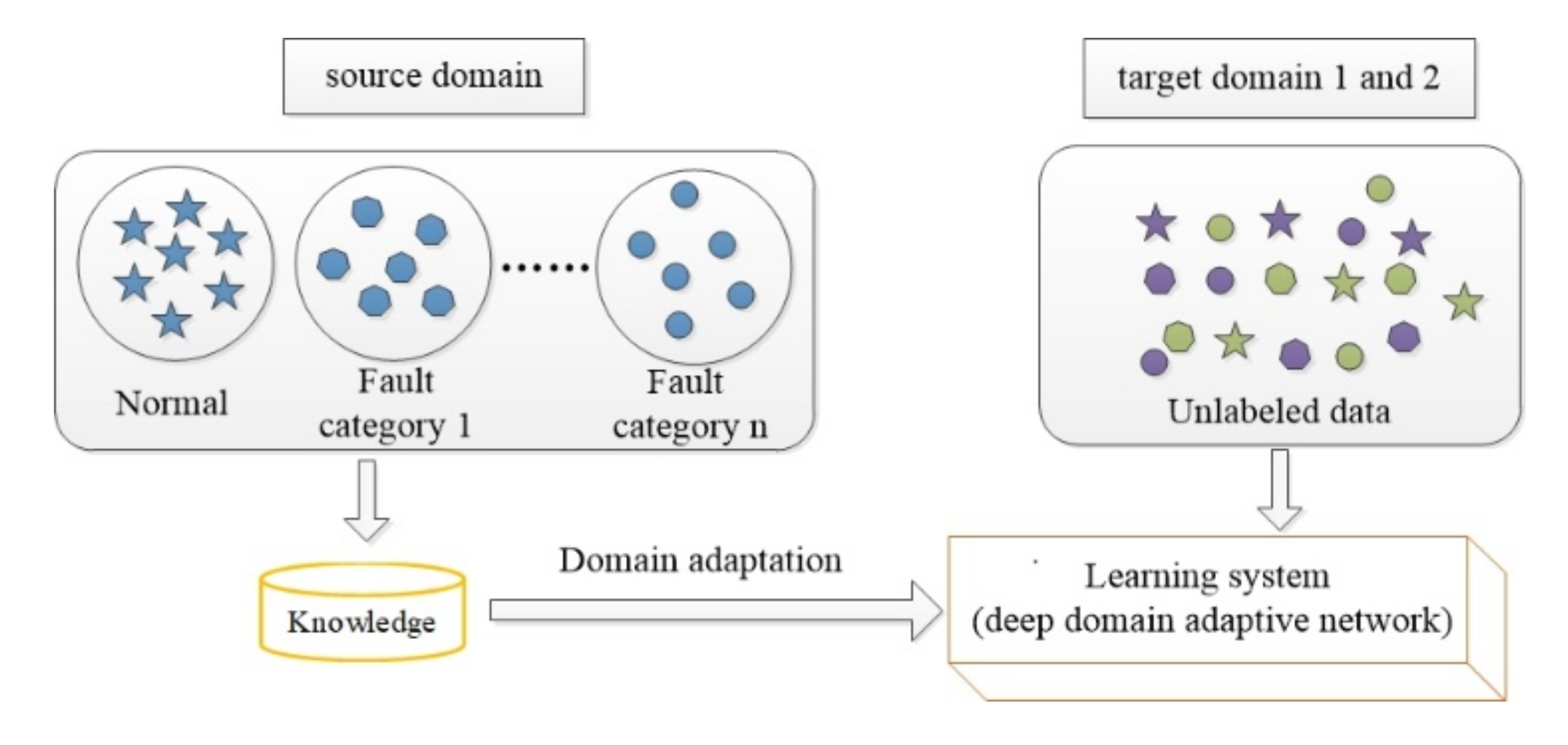
1. Introduction
- (1)
- The 1D-MSDAN model is proposed for the fault diagnosis of motor bearings under different working conditions. Different domain-invariant features are learned from multi-scale convolutional neural networks, and the distribution discrepancy can thus be minimized by multi-scale and multi-level feature adaptation; in addition, the classifier adaptation bridges the source classifier and target classifier for further domain adaptation.
- (2)
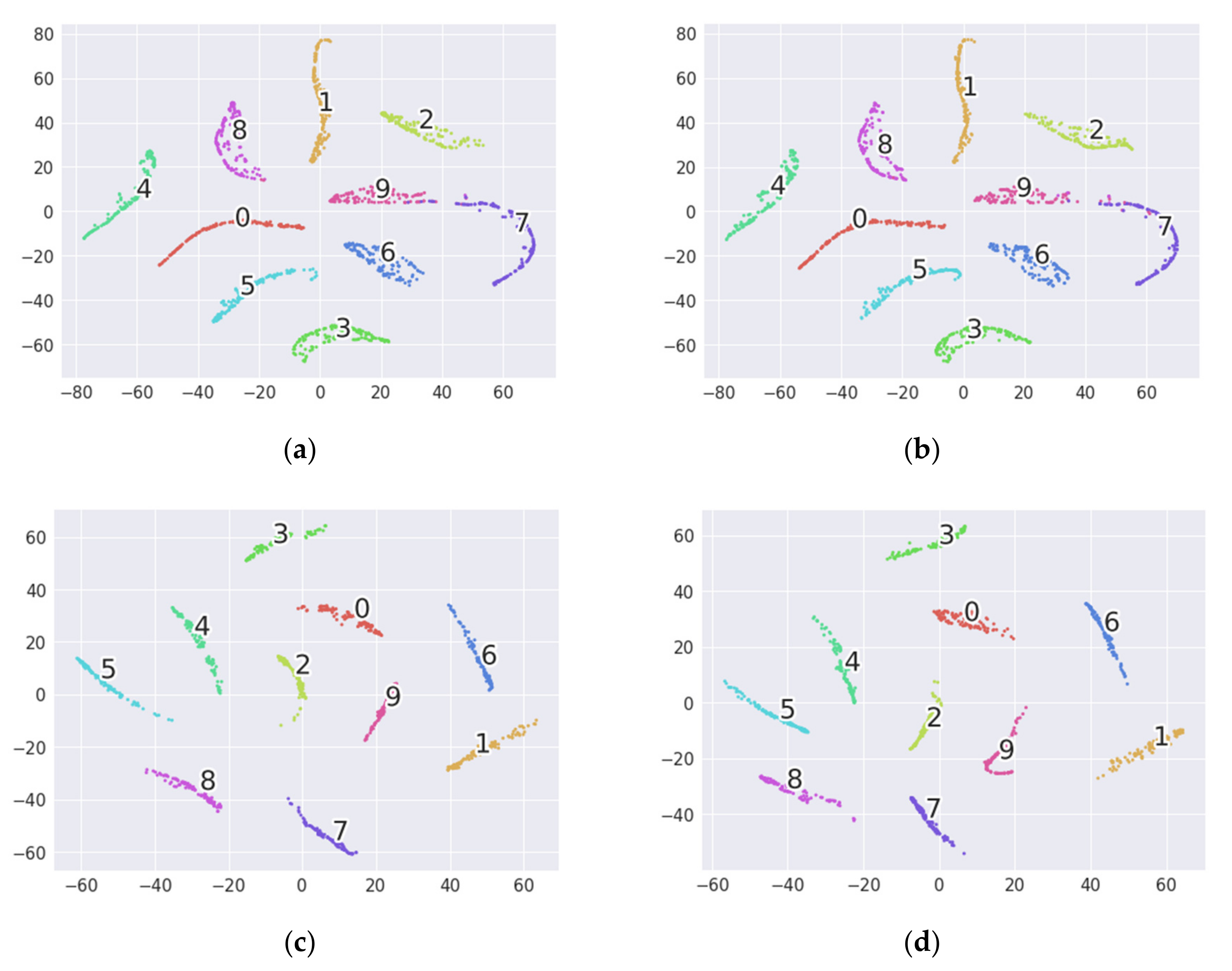
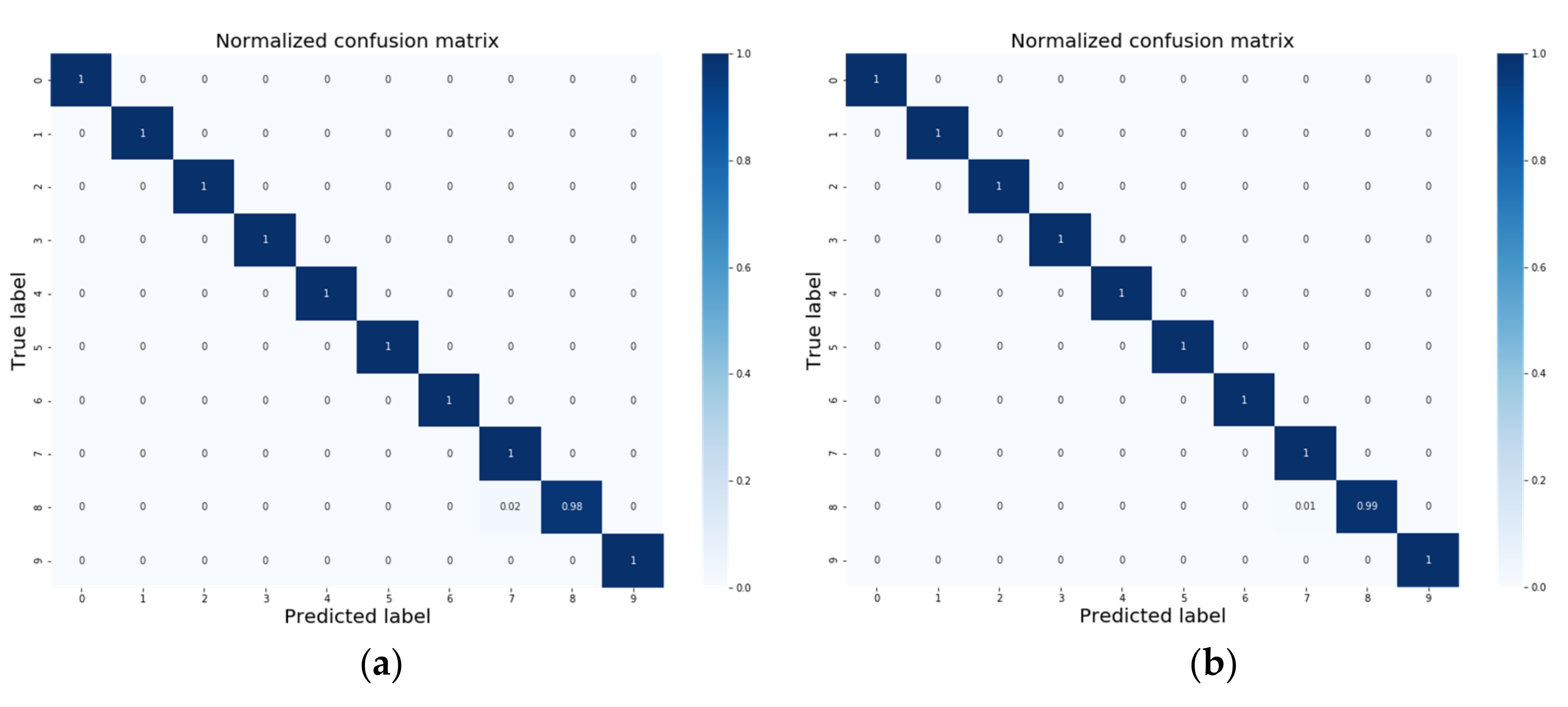
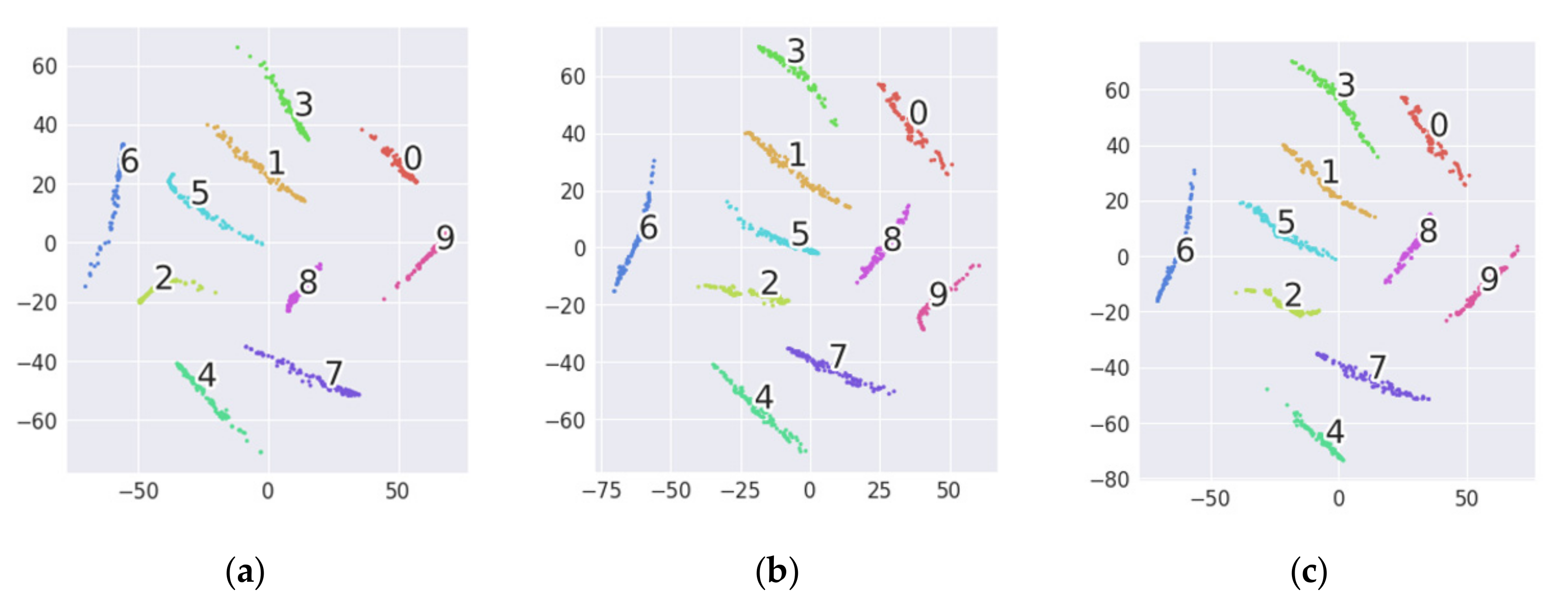
- The superiority of 1D-MSDAN is compared with some mainstream methods by implementing 12 transfer tasks on the Case Western Reserve University (CWRU) dataset, and feature visualization is used to further evaluate the superiority of the proposed 1D-MSDAN.
- (3)
- A transfer model is established to simultaneously solve the fault diagnosis problem of two unlabeled conditions in order to further improve the transfer efficiency. The transfer efficiency is increased by 50% while ensuring accuracy.
- (4)
- Different levels of Gaussian white noise are mixed with the data under testing to verify the effectiveness of 1D-MSDAN in real industrial scenarios.
2. Preliminary Knowledge of Some Concepts
2.1. Problem Formalization
2.2. Convolutional Neural Network
2.2.1. The Convolutional Layer
2.2.2. The Pooling Layer
2.2.3. The Fully Connected Layer
2.3. Maximum Mean Discrepancy
3. Proposed 1D-MSDAN for Bearing-Fault Diagnosis under Varying Working Conditions
3.1. Multi-Scale Feature Learning
3.2. Feature and Classification Adaptation
3.2.1. Multi-Scale and Multi-Level Feature Adaptation
3.2.2. Classifier Adaptation
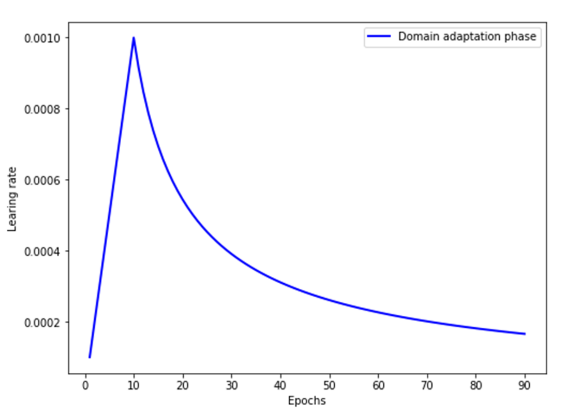
3.3. Optimization Objective and Training Strategy
- (1)
- Initial with random values.
- (2)
- Pre-training: update all the parameters by minimizing with the Adam optimization algorithm.
- (3)
- Repeat Step (2) until pre-training is finished.
- (4)
- Domain adaptation training: update by minimizing , and update by minimizing and .where α is the learning rate.
- (5)
- Repeat Step (4) until domain adaptation training is finished.
4. Case Study
4.1. Data Description and Parameter Setting
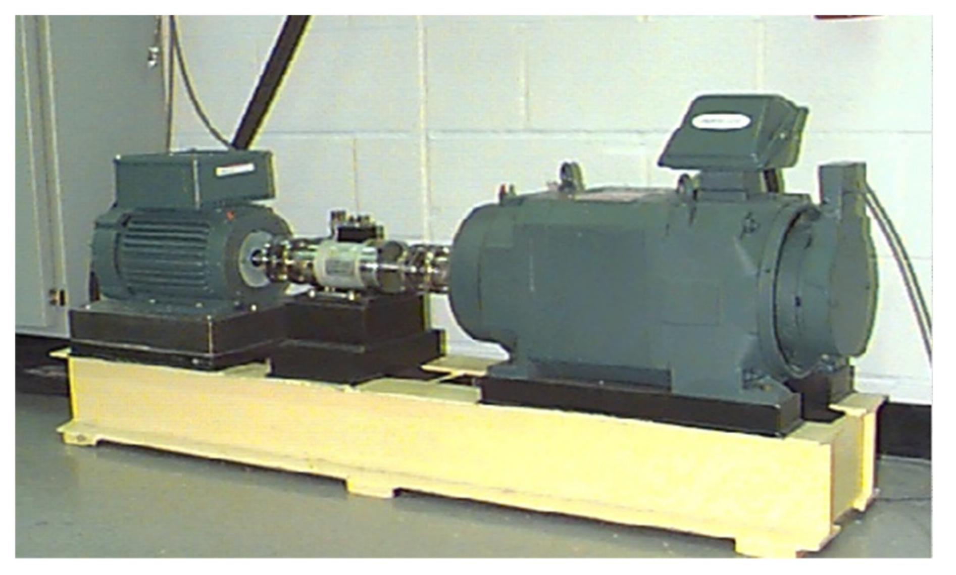
4.1.1. Data Description
4.1.2. Parameter Setting
4.2. Comparison with Other Transfer Learning Methods
- Ensemble TICNN: Zhang et al. [23] proposed TICNN, inspired by AdaBN [39]. TICNN replaces the batch normalization (BN) statistics from the source data with those from the target data to reduce the distribution discrepancy. In addition, Ensemble TICNN adds ensemble learning to improve the stability of the algorithm.
- SF-SOF-HKL: Inspired by moment discrepancy and Kullback-Leibler (KL) divergence, Qian et al. [26] proposed using high-order KL (HKL) divergence to align the high-order moments of the domain-specific distributions. Sparse filtering with HKL divergence (SF-HKL) can learn both discriminative and shared features between the source and target domains. Besides, Qian et al. validated that softmax regression with HKL divergence (SOF-HKL) can further improve performance.
- DACNN: Zhang et al. [24] proposed DACNN, which consists of three parts: a source feature extractor, a target feature extractor, and a label classifier. Like our approach, DACNN uses a two-stage training process: First, it uses pre-training to obtain the fault discriminative features. Then, the target feature extractor is trained to minimize the squared MMD. Different from in other domain adaptation models, the layers between the source and target feature extractor are partially untied in the training.
- WDMAN: Zhang et al. [25] proposed an adversarial training strategy for Multi-Adversarial networks guided by the Wasserstein distance to learn the domain-invariant features between the source and target domains. This method is inspired by the Generative Adversarial Network (GAN) [40], and its purpose is to learn a generator to generate fake images that are indistinguishable from real images.
4.3. Verification of Multi-Target Domain Adaptation
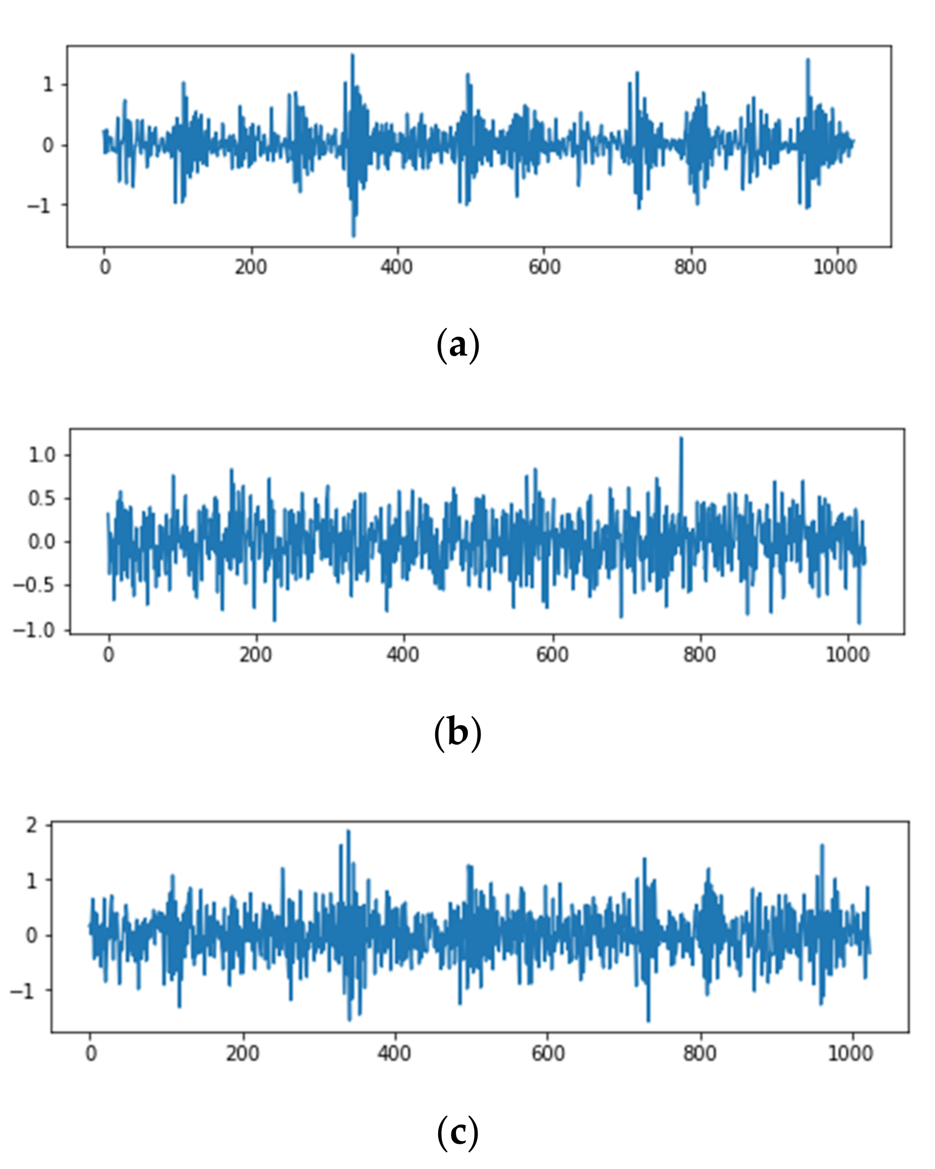
4.4. Verification of Real Industrial Scenarios
5. Conclusions
Author Contributions
Funding
Conflicts of Interest
References
- Cerrada, M.; Sanchez, R.V.; Li, C.; Pacheco, F.; Cabrera, D.; Oliveira, J.V.D.; Vasquez, R. A review on data-driven fault severity assessment in rolling bearings. Mech. Syst. Signal Process. 2018, 99, 169–196. [Google Scholar] [CrossRef]
- Georgoulas, G.; Loutas, T.; Stylios, C.D.; Kostopoulos, V. Bearing fault detection based on hybrid ensemble detector and empirical mode decomposition. Mech. Syst. Signal Process. 2013, 41, 510–525. [Google Scholar] [CrossRef]
- Hoang, D.T.; Kang, H.J. A survey on Deep Learning based bearing fault diagnosis. Neurocomputing 2019, 335, 327–335. [Google Scholar] [CrossRef]
- Ince, T.; Kiranyaz, S.; Eren, L.; Askar, M.; Gabbouj, M. Real-time motor fault detection by 1-d convolutional neural networks. IEEE Trans. Ind. Electron. 2016, 63, 7067–7075. [Google Scholar] [CrossRef]
- Wen, L.; Li, X.; Gao, L.; Zhang, Y. A new convolutional neural network-based data-driven fault diagnosis method. IEEE Trans. Ind. Electron. 2018, 65, 5990–5998. [Google Scholar] [CrossRef]
- Wang, J.; Li, S.; Han, B.; An, Z.; Ji, S. Generalization of deep neural networks for imbalanced fault classification of machinery using generative adversarial networks. IEEE Access 2019, 7, 111168–111180. [Google Scholar] [CrossRef]
- Mao, W.; Liu, Y.; Ding, L.; Li, Y. Imbalanced Fault Diagnosis of Rolling Bearing Based on Generative Adversarial Network: A Comparative Study. IEEE Access 2019, 7, 9515–9530. [Google Scholar] [CrossRef]
- Ma, S.; Liu, W.; Cai, W.; Shang, Z.; Liu, G. Lightweight Deep Residual CNN for Fault Diagnosis of Rotating Machinery Based on Depthwise Separable Convolutions. IEEE Access 2019, 7, 57023–57036. [Google Scholar] [CrossRef]
- Gan, M.; Wang, C.; Zhu, C.A. Construction of hierarchical diagnosis network based on deep learning and its application in the fault pattern recognition of rolling element bearings. Mech. Syst. Signal Process. 2016, 72, 92–104. [Google Scholar] [CrossRef]
- Hao, S.; Ge, F.X.; Li, Y.; Jiang, J. Multisensor bearing fault diagnosis based on one-dimensional convolutional long short-term memory networks. Measurement 2020, 159, 107802. [Google Scholar] [CrossRef]
- Pan, S.J.; Yang, Q. A survey on transfer learning. IEEE Trans. Knowl. Data Eng. 2010, 22, 1345–1359. [Google Scholar] [CrossRef]
- Pan, S.J.; Tsang, I.W.; Kwok, J.T.; Yang, Q. Domain adaptation via transfer component analysis. IEEE Trans. Neural Netw. 2011, 22, 199–210. [Google Scholar] [CrossRef] [PubMed]
- Long, M.; Wang, J.; Ding, G.; Sun, J.; Yu, P.S. Transfer feature learning with joint distribution adaptation. In Proceedings of the IEEE International Conference on Computer Vision, Sydney, Australia, 1–8 December 2013; pp. 2200–2207. [Google Scholar]
- Sun, B.; Saenko, K. Subspace distribution alignment for unsupervised domain adaptation. In Proceedings of the British Machine Vision Conference 2015, Swansea, UK, 7–10 September 2015; pp. 24.1–24.10. [Google Scholar]
- Shao, M.; Kit, D.; Fu, Y. Generalized transfer subspace learning through low-rank constraint. Int. J. Comput. Vis. 2014, 109, 74–93. [Google Scholar] [CrossRef]
- Long, M.; Cao, Y.; Wang, J.; Jordan, M.I. Learning transferable features with deep adaptation networks. In Proceedings of the International Conference on Machine learning, Lille, France, 6–11 July 2015; pp. 97–105. [Google Scholar]
- Long, M.; Zhu, H.; Wang, J.; Jordan, M.I. Deep transfer learning with joint adaptation networks. In Proceedings of the International Conference on Machine Learning, Sydney, Australia, 6–11 August 2017; pp. 2208–2217. [Google Scholar]
- Sun, B.; Saenko, K. Deep coral: Correlation alignment for deep domain adaptation. In Proceedings of the European Conference Computer Vision, Amsterdam, The Netherlands, 8–16 October 2016; pp. 443–450. [Google Scholar]
- Long, M.; Cao, Y.; Cao, Z.; Wang, J.; Jordan, M.I. Transferable Representation Learning with Deep Adaptation Networks. IEEE Trans. Pattern Anal. Mach. Intell. 2019, 41, 3071–3085. [Google Scholar] [CrossRef] [PubMed]
- Li, X.; Zhang, W.; Ding, Q.; Sun, J.Q. Multi-layer domain adaptation method for rolling bearing fault diagnosis. Signal Process. 2019, 157, 180–197. [Google Scholar] [CrossRef]
- Zhu, J.; Chen, N.; Shen, C. A New Deep Transfer Learning Method for Bearing Fault Diagnosis under Different Working Conditions. IEEE Sens. J. 2020, 20, 8394–8840. [Google Scholar] [CrossRef]
- Zhang, W.; Peng, G.; Li, C.; Chen, Y.; Zhang, Z. A new deep learning model for fault diagnosis with good anti-noise and domain adaptation ability on raw vibration signals. Sensors 2017, 17, 425. [Google Scholar] [CrossRef] [PubMed]
- Zhang, W.; Li, C.; Peng, G.; Chen, Y.; Zhang, Z. A deep convolutional neural network with new training methods for bearing fault diagnosis under noisy environment and different working load. Mech. Syst. Signal Process. 2018, 100, 439–453. [Google Scholar] [CrossRef]
- Zhang, B.; Li, W.; Li, X.; Ng, S. Intelligent Fault Diagnosis Under Varying Working Conditions Based on Domain Adaptive Convolutional Neural Networks. IEEE Access 2018, 6, 66367–66384. [Google Scholar] [CrossRef]
- Zhang, M.; Wang, D.; Lu, W.; Yang, J.; Li, Z.; Liang, B. A Deep Transfer Model with Wasserstein Distance Guided Multi-Adversarial Networks for Bearing Fault Diagnosis under Different Working Conditions. IEEE Access 2019, 7, 65303–65318. [Google Scholar] [CrossRef]
- Qian, W.; Li, S.; Wang, J. A New Transfer Learning Method and its Application on Rotating Machine Fault Diagnosis under Variant Working Conditions. IEEE Access 2018, 6, 69907–69917. [Google Scholar] [CrossRef]
- Long, M.; Zhu, H.; Wang, J.; Jordan, M.I. Unsupervised Domain Adaptation with Residual Transfer Networks. In Proceedings of the Neural Information Processing Systems (NIPS), Barcelona, Spain, 5–10 December 2016; pp. 136–144. [Google Scholar]
- Zhu, Y.; Zhuang, F.; Wang, J.; Chen, J.; Shi, Z.; Wu, W.; He, Q. Multi-representation adaptation network for cross-domain image classification. Neural Networks 2019, 119, 214–221. [Google Scholar] [CrossRef] [PubMed]
- Krizhevsky, A.; Sutskever, I.; Hinton, G.E. Imagenet classification with deep convolutional neural networks. In Proceedings of the Advances in Neural Information Processing Systems, Harrahs and Harveys, Tahoe City, CA, USA, 3–6 December 2012; pp. 1097–1105. [Google Scholar]
- Jiang, Q.; Chang, F.; Sheng, B. Bearing Fault Classification Based on Convolutional Neural Network in Noise Environment. IEEE Access 2019, 7, 69795–69807. [Google Scholar] [CrossRef]
- Goodfellow, I.; Bengio, Y.; Courville, A. Deep Learning; The MIT Press: Cambridge, MA, USA, 2016; pp. 203–206. [Google Scholar]
- Fukumizu, K.; Gretton, A.; Sun, X.; Schölkopf, B. Kernel measures of conditional dependence. In Proceedings of the Advances in Neural Information Processing Systems, Vancouver, BC, Canada, 3–6 December 2008; pp. 489–496. [Google Scholar]
- Hinton, G.; Srivastava, N.; Krizhevsky, A.; Sutskever, I.; Salakhutdinov, R. Improving neural networks by preventing co-adaptation of feature detectors. arXiv 2012, arXiv:1207.0580. [Google Scholar]
- Ioffe, S.; Szegedy, C. Batch normalization: Accelerating deep network training by reducing internal covariate shift. arXiv 2015, arXiv:1502.03167. [Google Scholar]
- Kingma, D.P.; Ba, J. Adam: A method for stochastic optimization. arXiv 2014, arXiv:1412.6980. [Google Scholar]
- Smith, W.A.; Randall, R.B. Rolling element bearing diagnostics using the Case Western Reserve University data: A benchmark study. Mech. Syst. Signal Process. 2015, 64, 100–131. [Google Scholar] [CrossRef]
- He, K.; Zhang, X.; Ren, S.; Sun, J. Deep Residual Learning for Image Recognition. In Proceedings of the 2016 IEEE Conference on Computer Vision and Pattern Recognition (CVPR), Las Vegas, NV, USA, 27–30 June 2016; pp. 770–778. [Google Scholar]
- Ganin, Y.; Ustinova, E.; Ajakan, H.; Germain, P.; Larochelle, H.; Laviolette, F.; Marchand, M.; Lempitsky, V. Domain-adversarial training of neural networks. J. Mach. Learn. Res. 2016, 17, 2096–2030. [Google Scholar]
- Li, Y.; Wang, N.; Shi, J.; Hou, X.; Liu, J. Adaptive batch normalization for practical domain adaptation. Pattern Recognit. 2018, 80, 109–117. [Google Scholar] [CrossRef]
- Goodfellow, I.; Pouget-Abadie, J.; Mirza, M.; Xu, B.; Warde-Farley, D.; Ozair, S.; Courville, A.; Bengio, Y. Generative adversarial nets. In Proceedings of the Advances in Neural Information Processing Systems, Montreal, QC, Canada, 8–13 December 2014; pp. 2672–2680. [Google Scholar]
- Van der Maaten, L.; Hinton, G. Visualizing data using t-SNE. J. Mach. Learn. Res. 2008, 9, 2579–2605. [Google Scholar]


| Module | Layer | Parameters | Activation Function | Output Size |
|---|---|---|---|---|
| Input | Input | / | / | 1024 × 1 |
| Feature extractor 1 | Convolution 1_1 | Kernel_size = 20 × 1, stride = 2 | ReLU | 512 × 16 |
| Max pooling 1_1 | Kernel_size = 2 × 1, stride = 2 | / | 256 × 16 | |
| Convolution 1_2 | Kernel_size = 5 × 1, stride = 1 | ReLU | 256 × 32 | |
| Max pooling 1_2 | Kernel_size = 2 × 1, stride = 2 | / | 128 × 32 | |
| Convolution 1_3 | Kernel_size = 5 × 1, stride = 1 | ReLU | 128 × 64 | |
| Max pooling 1_3 | Kernel_size = 2 × 1, stride = 2 | / | 64 × 64 | |
| Convolution 1_4 | Kernel_size = 5 × 1, stride = 1 | ReLU | 64 × 64 | |
| Average pooling 1_4 | Kernel_size = 2 × 1, stride = 2 | / | 32 × 64 | |
| Feature extractor 2 | Convolution 2_1 | Kernel_size = 20 × 1, stride = 2 | ReLU | 512 × 16 |
| Max pooling 2_1 | Kernel_size = 2 × 1, stride = 2 | / | 256 × 16 | |
| Convolution 2_2 | Kernel_size = 3 × 1, stride = 1 | ReLU | 256 × 32 | |
| Max pooling 2_2 | Kernel_size = 2 × 1, stride = 2 | / | 128 × 32 | |
| Convolution 2_3 | Kernel_size = 3 × 1, stride = 1 | ReLU | 128 × 64 | |
| Max pooling 2_3 | Kernel_size = 2 × 1, stride = 2 | / | 64 × 64 | |
| Convolution 2_4 | Kernel_size = 3 × 1, stride = 1 | ReLU | 64 × 64 | |
| Average pooling 2_4 | Kernel_size = 2 × 1, stride = 2 | / | 32 × 64 | |
| Feature extractor 3 | Convolution 3_1 | Kernel_size = 20 × 1, stride = 2 | ReLU | 512 × 16 |
| Max pooling 3_1 | Kernel_size = 2 × 1, stride = 2 | / | 256 × 16 | |
| Convolution 3_2 | Kernel_size = 1 × 1, stride = 1 | ReLU | 256 × 32 | |
| Max pooling 3_2 | Kernel_size = 2 × 1, stride = 2 | / | 128 × 32 | |
| Convolution 3_3 | Kernel_size = 1 × 1, stride = 1 | ReLU | 128 × 64 | |
| Max pooling 3_3 | Kernel_size = 2 × 1, stride = 2 | / | 64 × 64 | |
| Convolution 3_4 | Kernel_size = 1 × 1, stride = 1 | ReLU | 64 × 64 | |
| Average pooling 3_4 | Kernel_size = 2 × 1, stride = 2 | / | 32 × 64 | |
| Classifier | Fully connected 1 | Weights = 64 × 96, bias = 1024 | ReLU | 1014 × 1 |
| Fully connected 2 | Weights = 1024 × 10, bias = 10 | Softmax | 10 × 1 |
| Domain | Operation Conditions | Number of Samples | Number of Categories |
|---|---|---|---|
| A | 0 HP | 5000 | 10 |
| B | 1 HP | 5000 | 10 |
| C | 2 HP | 5000 | 10 |
| D | 3 HP | 5000 | 10 |
| Ensemble TICNN [23] | SF-SOF-HKL [26] | DACNN [24] | WDMAN [25] | 1D-MSDAN | |
|---|---|---|---|---|---|
| A→B | _ | 99.80% | _ | 99.73% | 100.00% |
| A→C | _ | 87.56% | _ | 99.67% | 100.00% |
| A→D | _ | 99.70% | _ | 100.00% | 100.00% |
| B→A | _ | 99.86% | _ | 99.13% | 99.95% |
| B→C | 99.50% | 99.59% | 100.00% | 100.00% | 100.00% |
| B→D | 91.10% | 95.50% | 99.69% | 99.93% | 100.00% |
| C→A | _ | 88.50% | _ | 98.53% | 99.90% |
| C→B | 97.60% | 99.23% | 100.00% | 99.80% | 100.00% |
| C→D | 99.40% | 98.16% | 99.90% | 100.00% | 100.00% |
| D→A | _ | 100.00% | _ | 98.07% | 99.86% |
| D→B | 90.20% | 95.17% | 97.98% | 98.27% | 99.90% |
| D→C | 98.7% | 97.81% | 100.00% | 99.53% | 100.00% |
| AVG | _ | 96.74% | _ | 99.39% | 99.97% |
| Task | Parameter | Target 1 | Target 2 |
|---|---|---|---|
| A→B + C | λ = 1, γ = 0.2 | 100.00% | 100.00% |
| B→A + C | λ = 1, γ = 0.2 | 99.90% | 100.00% |
| B→C + D | λ = 1, γ = 0.2 | 100.00% | 100.00% |
| C→B + A | λ = 1, γ = 0.2 | 99.80% | 99.80% |
| C→B + D | λ = 1, γ = 0.2 | 100.00% | 100.00% |
| D→B + C | λ = 1, γ = 0.2 | 99.30% | 100.00% |
| Task | SNR = 1 | SNR = 2 | SNR = 3 | No Noise |
|---|---|---|---|---|
| A→B | 98.76% | 99.70% | 99.70% | 100.00% |
| A→C | 99.60% | 99.85% | 99.90% | 100.00% |
| A→D | 99.70% | 99.68% | 99.92% | 100.00% |
| B→A | 98.50% | 99.30% | 99.10% | 99.70% |
| B→C | 99.68% | 99.95% | 99.95% | 100.00% |
| B→D | 99.01% | 99.70% | 99.85% | 100.00% |
| C→A | 99.08% | 99.34% | 99.40% | 99.90% |
| C→B | 97.44% | 97.20% | 97.20% | 100.00% |
| C→D | 100.00% | 99.80% | 100.00% | 100.00% |
| D→A | 99.14% | 99.60% | 99.70% | 99.70% |
| D→B | 97.24% | 97.10% | 97.10% | 99.90% |
| D→C | 100.00% | 100.00% | 99.85% | 100.00% |
| AVG | 99.01% | 99.27% | 99.31% | 99.97% |
Publisher’s Note: MDPI stays neutral with regard to jurisdictional claims in published maps and institutional affiliations. |
© 2020 by the authors. Licensee MDPI, Basel, Switzerland. This article is an open access article distributed under the terms and conditions of the Creative Commons Attribution (CC BY) license (http://creativecommons.org/licenses/by/4.0/).
Share and Cite
Wang, K.; Zhao, W.; Xu, A.; Zeng, P.; Yang, S. One-Dimensional Multi-Scale Domain Adaptive Network for Bearing-Fault Diagnosis under Varying Working Conditions. Sensors 2020, 20, 6039. https://doi.org/10.3390/s20216039
Wang K, Zhao W, Xu A, Zeng P, Yang S. One-Dimensional Multi-Scale Domain Adaptive Network for Bearing-Fault Diagnosis under Varying Working Conditions. Sensors. 2020; 20(21):6039. https://doi.org/10.3390/s20216039
Chicago/Turabian StyleWang, Kai, Wei Zhao, Aidong Xu, Peng Zeng, and Shunkun Yang. 2020. "One-Dimensional Multi-Scale Domain Adaptive Network for Bearing-Fault Diagnosis under Varying Working Conditions" Sensors 20, no. 21: 6039. https://doi.org/10.3390/s20216039
APA StyleWang, K., Zhao, W., Xu, A., Zeng, P., & Yang, S. (2020). One-Dimensional Multi-Scale Domain Adaptive Network for Bearing-Fault Diagnosis under Varying Working Conditions. Sensors, 20(21), 6039. https://doi.org/10.3390/s20216039