Power-Saving Design of Radio Frequency Identification Sensor Networks in Bus Seatbelt Monitoring Systems


Abstract
1. Introduction
2. Power-Saving Design in Hardware Systems
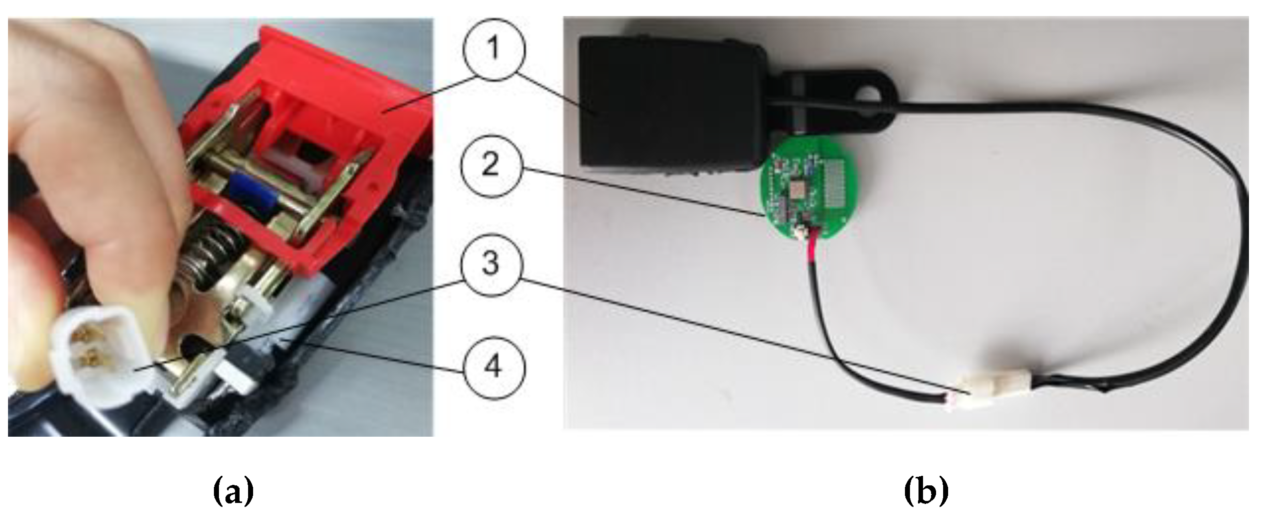
2.1. Overview
- (1)
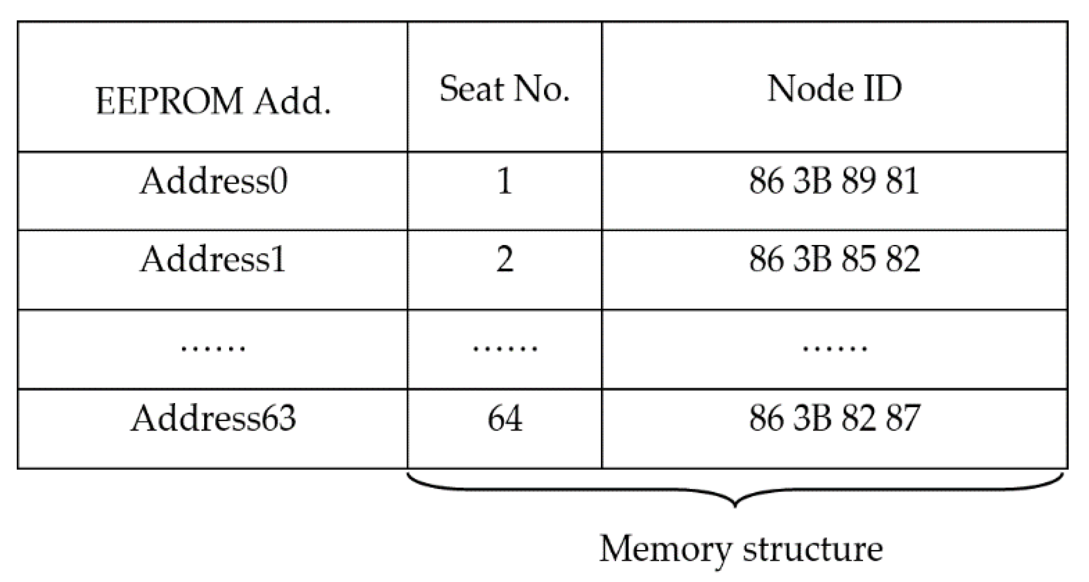
- Node Registration:
- Turn concentrator power on.
- Press “plus” key and make the data counter (i.e., digital tube) display “01”.
- Press the node registration key and then fasten the seat safety belt (i.e., power on) to make node transmit registration ID.
- If the data counter in the concentrator adds one to “02”, the node registration is successful.
- Repeat these procedures until all of the 64-seatbelt node ID registration is completed.
- Press the “reset key” to enter into normal mode.
- (2)
- Normal Mode Control:
- When the data counter displays “00”, the concentrator enters into its normal mode.
- In the normal mode, the node will transmit seatbelt state data when it is buckled. The concentrator will receive the state data and check state data integrity.
- If the state data belongs to this bus, it will be sent to RF controller. Otherwise, it will be cleared.
- (3)
- Node Replacement:
- Adjust the data counter to match the seat number if modification is required.
- Press the new node registration key, and then fasten the seatbelt to transmit registration ID.
- If the data counter in the concentrator adds one, the replacement of the new node is completed.
- Press “Reset” key to enter into the normal mode.
2.2. Low-Power Design in Hardware Systems
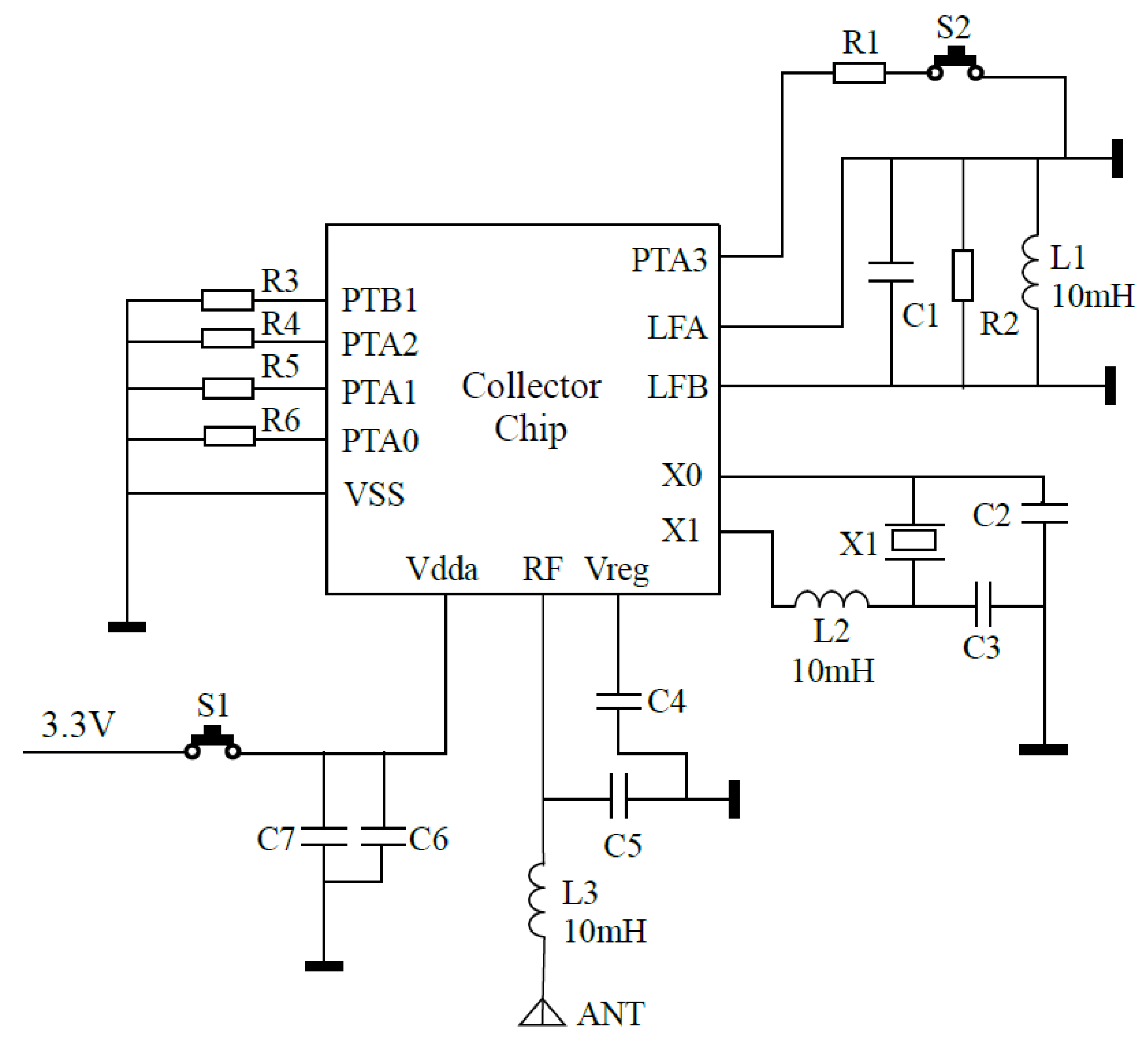
2.2.1. Use of Low-Power Devices
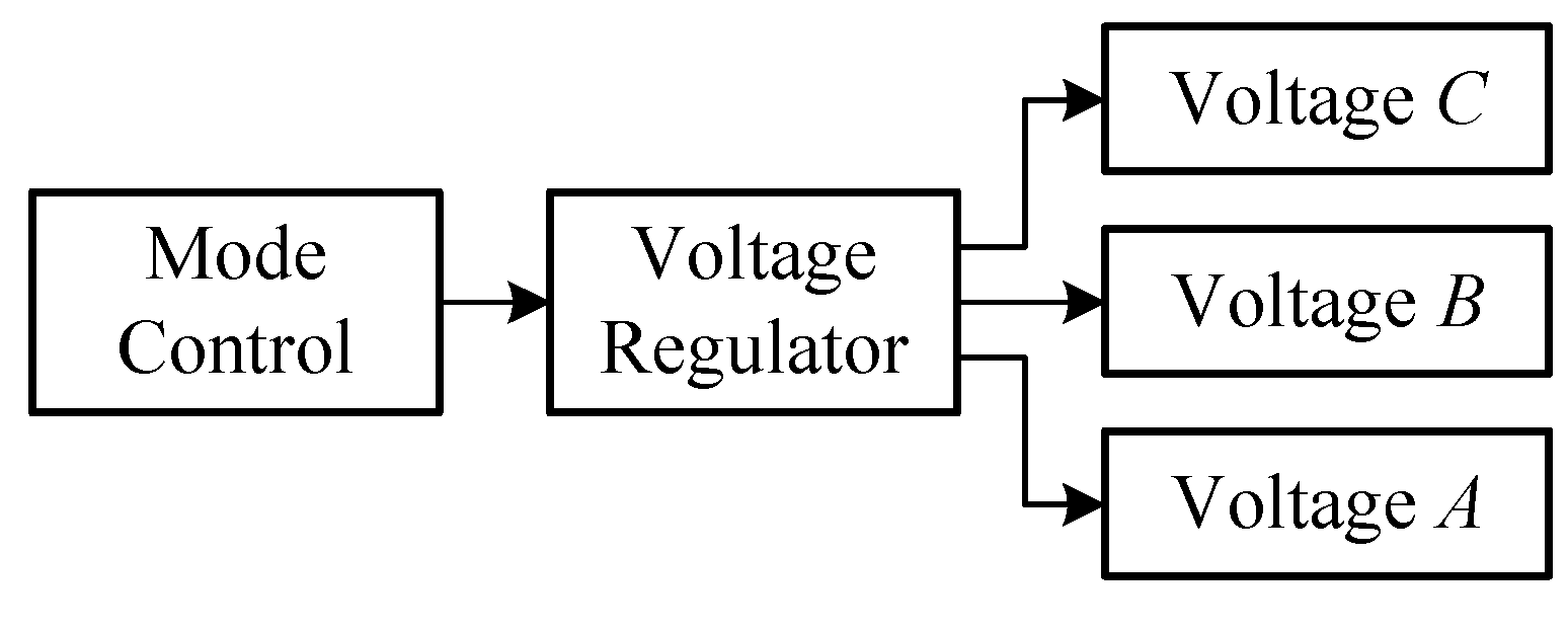
2.2.2. Low-Power Supply Control
2.2.3. Low-Power Frequency Control
3. Power-Saving Design of the Software System
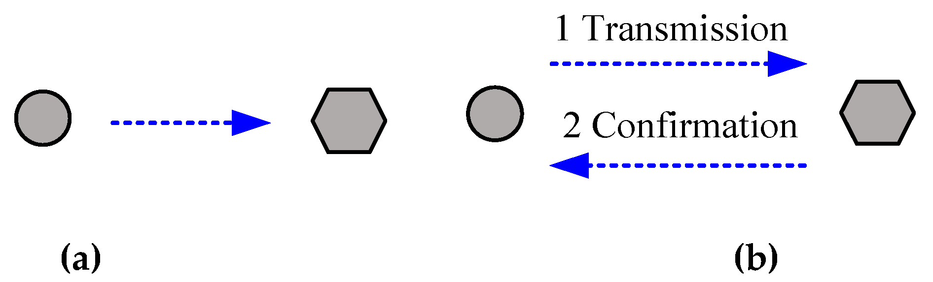
3.1. Selection of Node Communication Mode
3.2. Sending Period of the Node
3.2.1. Real-Time Transmission State
3.2.2. Periodic Transmission State
3.2.3. Determination of Transmission Duration
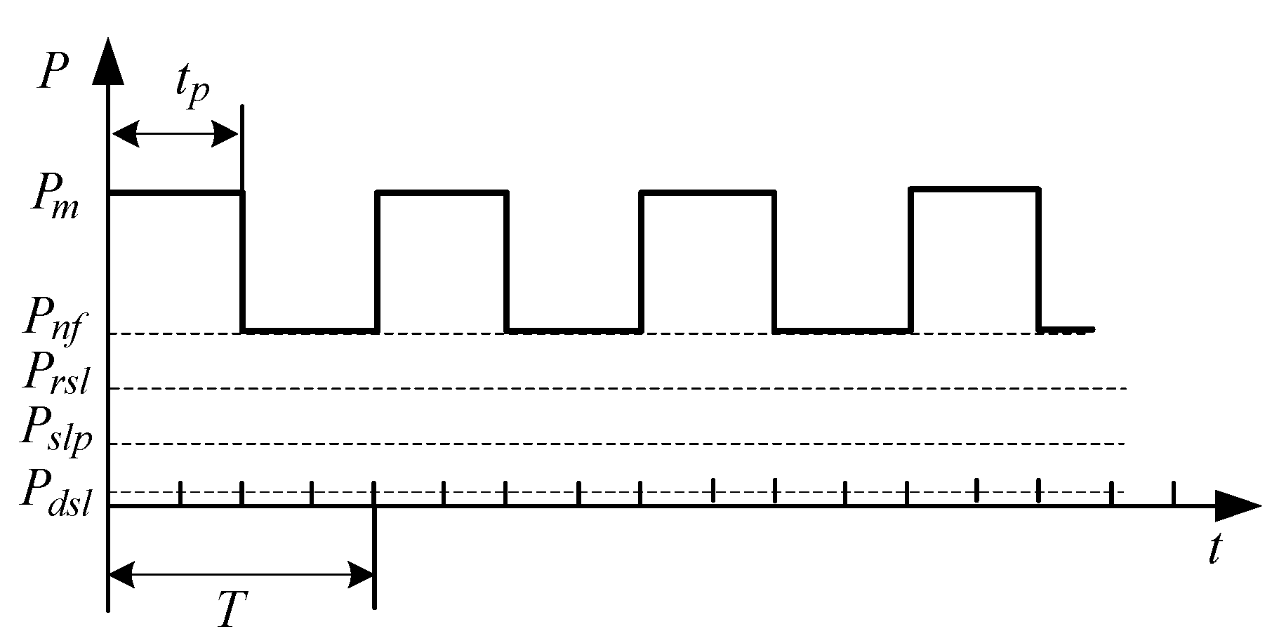
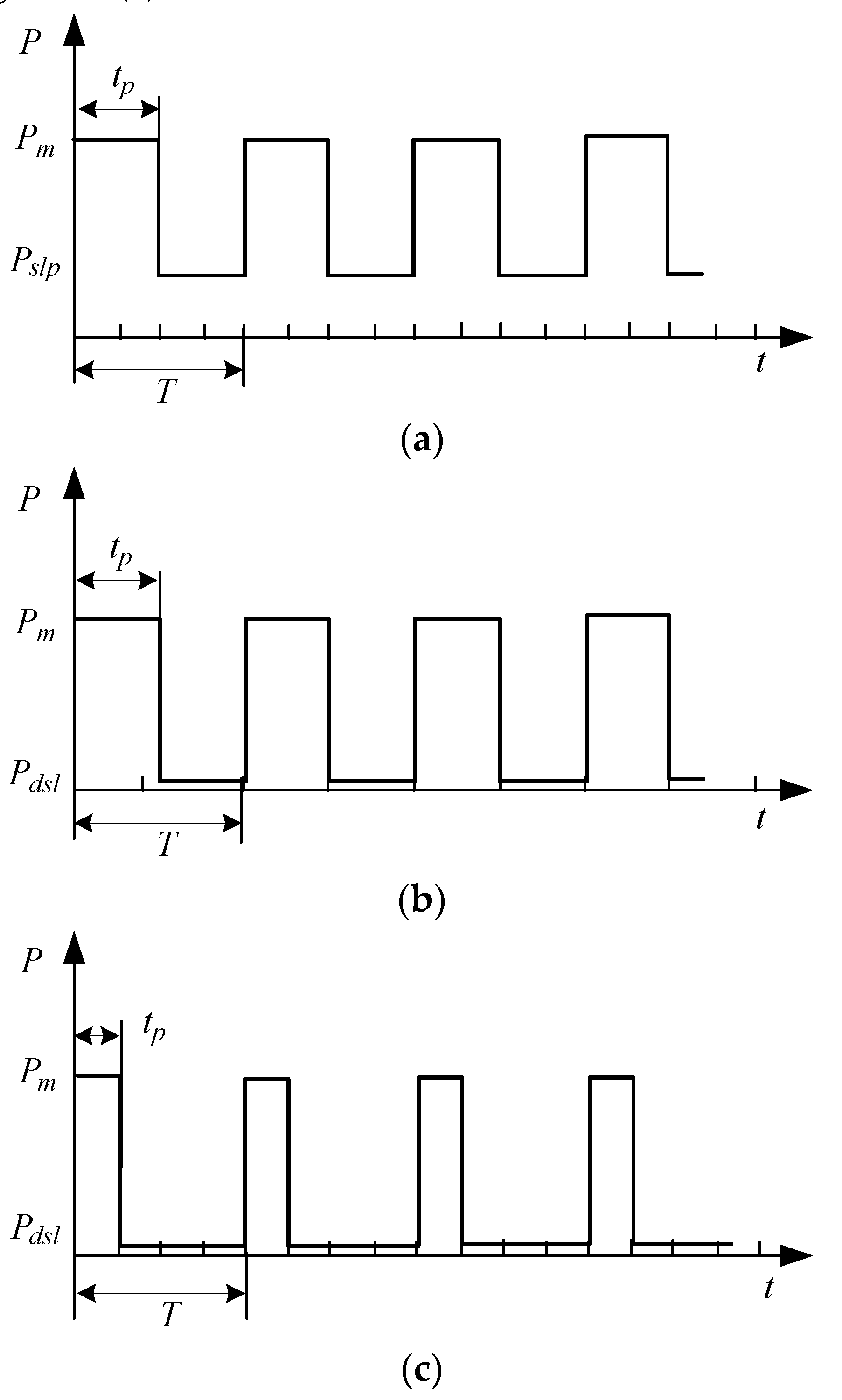
3.3. Selection of Sleep Mode
4. System Performance Testing
4.1. System Running Testing
4.2. Node Battery Current Consumption
5. Conclusions
Author Contributions
Funding
Conflicts of Interest
References
- Peng, J.; Feng, C. 3D coverage scheme based on hibernation of redundant nodes and phased waking up strategy for wireless sensor networks. J. Electron. Inf. Technol. 2009, 31, 2807–2812. [Google Scholar]
- Kai, Y.; Zhijun, X.; Guang, J.; Jiangbo, Q. Design and implementation of low-power wireless sensor net-work node. In Proceedings of the IEEE Conference on Vehicular Technology (VTC), Sydney, NSW, Australia, 4–7 June 2017. [Google Scholar]
- Ziwei, Y.; Zhijiu, Z.; Jia, Y. Design and optimization of the off mode of low power MCU. Microelectron. Comput. 2017, 34, 26–30. [Google Scholar]
- Behrouj, A.R.; Ghorbani, A.R.; Ghaznavi-Ghoushchi, M.B.; Jalali, M. A low-power CMOS transceiver in 130 nm for wireless sensor network applications. Wirel. Pers. Commun. 2019, 106, 1015–1039. [Google Scholar] [CrossRef]
- Radfar, M.; Nakhlestani, A.; Le Viet, H.; Desai, A. Battery management technique to reduce standby energy consumption in ultra-low power IoT and sensory applications. IEEE Trans. Circuits Syst. I Regul. Pap. 2020, 67, 336–345. [Google Scholar] [CrossRef]
- Kaushik, K.; Mishra, D.; De, S.; Chowdhury, K.R.; Heinzelman, W. Low-cost wake-up receiver for RF energy harvesting wireless sensor networks. IEEE Sens. J. 2016, 16, 6270–6278. [Google Scholar] [CrossRef]
- Oller, J.; Demirkol, I.; Casademont, J.; Paradells, J.; Gamm, G.U.; Reindl, L. Has time come to switch from duty-cycled MAC protocols to wake-up radio for wireless sensor networks? IEEE/ACM Trans. Netw. 2015, 24, 674–687. [Google Scholar] [CrossRef]
- Piyare, R.; Murphy, A.L.; Kiraly, C.; Tosato, P.; Brunelli, D. Ultra low power wake-up radios: A hardware and networking survey. IEEE Commun. Surv. Tutor. 2017, 19, 2117–2157. [Google Scholar] [CrossRef]
- Xiang, H.; Dan, L.; Jianhong, L.; Xiang, Y. Design of active RFID low-power tag based on DFM. Microelectron. Comput. 2014, 2, 171–173. [Google Scholar]
- Zhuojin, P.; Jilei, L.; Zhen, L. Design and implementation of low-power wireless sensor network nodes. Comput. Eng. Des. 2015, 36, 73–77. [Google Scholar]
- Ren, Z.; Zhao, Y.; Cao, H. Energy saving algorithm of zigbee network based on whole network dormancy. In Proceedings of the 2017 International Conference on Mechanical, Electronic, Control and Automation Engineering (MECAE 2017), Beijing, China, 25–26 March 2017; pp. 391–397. [Google Scholar]
- Jingxiang, L.; Wenlang, L. Quantization and energy optimization strategy of wireless sensor networks. J. Electron. Inf. Technol. 2020, 1, 1–7. [Google Scholar]
- Wei, L.; Jiali, Z. Design of a high-precision and low-power temperature acquisition system based on NB-IoT. Chin. J. Sens. Actuators. 2018, 31, 20–24. [Google Scholar]
- Abdal-Kadhim, A.M.; Leong, K.S. Electrical power flow of typical wireless sensor node based on energy harvesting approach. Int. J. Electron. Lett. 2018, 8, 17–27. [Google Scholar] [CrossRef]
- Shinghal, K.; Noor, A.; Srivastava, N.; Singh, R. Power measurements of wireless sensor networks node. Int. J. Comput. Eng. Sci. 2011, 1, 8–13. [Google Scholar] [CrossRef]
- Jurenoks, A. Method for node lifetime assessment in wireless sensor network with dynamic coordinator. In Proceedings of the 2015 IEEE 3rd Workshop on Advances in Information, Electronic and Electrical Engineering (AIEEE), At Riga, Latvia, 13–14 November 2015; pp. 1–5. [Google Scholar]
- Dey, N.; Ashour, A.S.; Shi, F.; Fong, S.J.; Sherratt, R.S. Developing residential wireless sensor networks for ECG healthcare monitoring. IEEE Trans. Consum. Electron. 2017, 63, 442–449. [Google Scholar] [CrossRef]
- Sundaravadivel, P.; Kougianos, E.; Mohanty, S.P.; Ganapathiraju, M.K. Everything you wanted to know about smart health care: Evaluating the different technologies and components of the internet of things for better health. IEEE Consum. Electron. Mag. 2017, 7, 18–28. [Google Scholar] [CrossRef]
- Lee, S.-Y.; Tsou, C.; Huang, P.-W. Ultra-high-frequency radio-frequency-identification baseband processor design for bio-signal acquisition and wireless transmission in healthcare system. IEEE Trans. Consum. Electron. 2019, 66, 77–86. [Google Scholar] [CrossRef]
- Sun, F.; Zhao, Z.; Fang, Z.; Chen, D.; Chen, X.; Xuan, Y. Design and implementation of an ultra low power health monitoring node for wireless body sensor network. In Proceedings of the 2013 Fourth International Conference on Digital Manufacturing & Automation, Qingdao, Shandong, China, 29–30 June 2013; pp. 417–422. [Google Scholar]
- Le, W. Application of wireless sensor network and RFID monitoring system in airport logistics. Int. J. Online Eng. 2018, 14, 89–103. [Google Scholar] [CrossRef]
- Xiaojun, M.; Shengbo, Z.; Bixi, X. Research on auto-test device of safety buckles in car. Mach. Tool Hydraul. 2006, 12, 158–160. [Google Scholar]
- Cotter, W.D. Seat Belt Status External Monitoring Apparatus and Method. U.S. Patent 7812716B1, 12 October 2010. [Google Scholar]
- Dexu, W.; Xiaolong, Z.; Yanzhao, W. Study on the effect of seat belt reminder for passenger cars in China. Beijing Automot. Eng. 2006, 2, 5–8. [Google Scholar]
- Yejian, T.; Songbai, J. Design of automatic safety belt reminder system for large bus seats. Mech. Electr. Eng. Technol. 2017, 46, 78–79. [Google Scholar]
- Hui, L.; Jianbiao, Z.; Chuang, L.; Song, Y.; Xuedong, L.; Ren, D.; Hong, G. Safety belt compulsory device based on speed limit. Int. Electr. Elem. 2011, 19, 141–144. [Google Scholar]
- Yano, I.H.; De Oliveira, V.C.; Becker, M.; Correa, A.S. Applying a hybrid polling approach by software implementation to extend the lifetime of a wireless sensor network. J. Comput. Sci. 2015, 11, 699–706. [Google Scholar] [CrossRef][Green Version]
- Rukpakavong, W.; Guan, L.; Phillips, I. Dynamic node lifetime estimation for wireless sensor networks. IEEE Sens. J. 2013, 14, 1370–1379. [Google Scholar] [CrossRef]
- Nan, L.; Wei, L. Research and simulation of sleeping schedule algorithm of wireless sensor networks. J. MinJiang Univ. 2008, 29, 72–76. [Google Scholar]
Publisher’s Note: MDPI stays neutral with regard to jurisdictional claims in published maps and institutional affiliations. |


| Working Mode | Clock Allocation Description |
|---|---|
| Operation | Turn on all clock sources. All circuits work normally. |
| Standby | HF and LF are on. MF is off. CPU and fixed cycle wake-up circuit are in standby state. When the set time is up, CPU is woken up, and enters the operation mode. |
| Sleep-receiving | MF is on. HF and LF are off. CPU is in sleep mode. RF receiving circuit is always on. Once the request signal of the upper level is detected, MCU will turn into operation mode. |
| General sleep | LF and MF is on. HF is off. CPU, flash and random-access memory (RAM) are in the hold state. Sensor group can be opened selectively. |
| Deep sleep | LF is on. MF and HF are off. Only service parameter register, real-time clock and wake-up module are serviced. |
| Chip Parameters | Operation Design | General Sleep Design | Deep Sleep Design | |
|---|---|---|---|---|
| Maximum launching voltage drop (V) | 0.10 | 0.10 | 0.10 | |
| Launching current (mA) | 7.60 | 10.00 | 10.00 | 10.00 |
| Sending interval (s) | 59.99 | 1.86 | 59.99 | 59.99 |
| Time of launching 16 bytes (ms) | 13.00 | 14.00 | 14.10 | 13.90 |
| Standby/sleeping current (uA) | 0.90 | 95.00 | 56.20 | 5.31 |
| Cycle current consumption (mAs) | 0.18 | 581.58 | 3.49 | 0.45 |
| Total service life (year) | 0.004 | 0.69 | 5.35 |
© 2020 by the authors. Licensee MDPI, Basel, Switzerland. This article is an open access article distributed under the terms and conditions of the Creative Commons Attribution (CC BY) license (http://creativecommons.org/licenses/by/4.0/).
Share and Cite
Sun, S.; Yang, W.; Wang, W. Power-Saving Design of Radio Frequency Identification Sensor Networks in Bus Seatbelt Monitoring Systems. Sensors 2020, 20, 5882. https://doi.org/10.3390/s20205882
Sun S, Yang W, Wang W. Power-Saving Design of Radio Frequency Identification Sensor Networks in Bus Seatbelt Monitoring Systems. Sensors. 2020; 20(20):5882. https://doi.org/10.3390/s20205882
Chicago/Turabian StyleSun, Sitong, Wen Yang, and Wilson Wang. 2020. "Power-Saving Design of Radio Frequency Identification Sensor Networks in Bus Seatbelt Monitoring Systems" Sensors 20, no. 20: 5882. https://doi.org/10.3390/s20205882
APA StyleSun, S., Yang, W., & Wang, W. (2020). Power-Saving Design of Radio Frequency Identification Sensor Networks in Bus Seatbelt Monitoring Systems. Sensors, 20(20), 5882. https://doi.org/10.3390/s20205882