A Shape Approximation for Medical Imaging Data


Abstract
:1. Introduction
2. Optimization Criteria
- Rotate by the following rotation matrix M with three radians :
- Furthermore, by translating and scaling by and , respectively, the general form of a cashew-shaped equation is represented bywhere and is defined in (4).
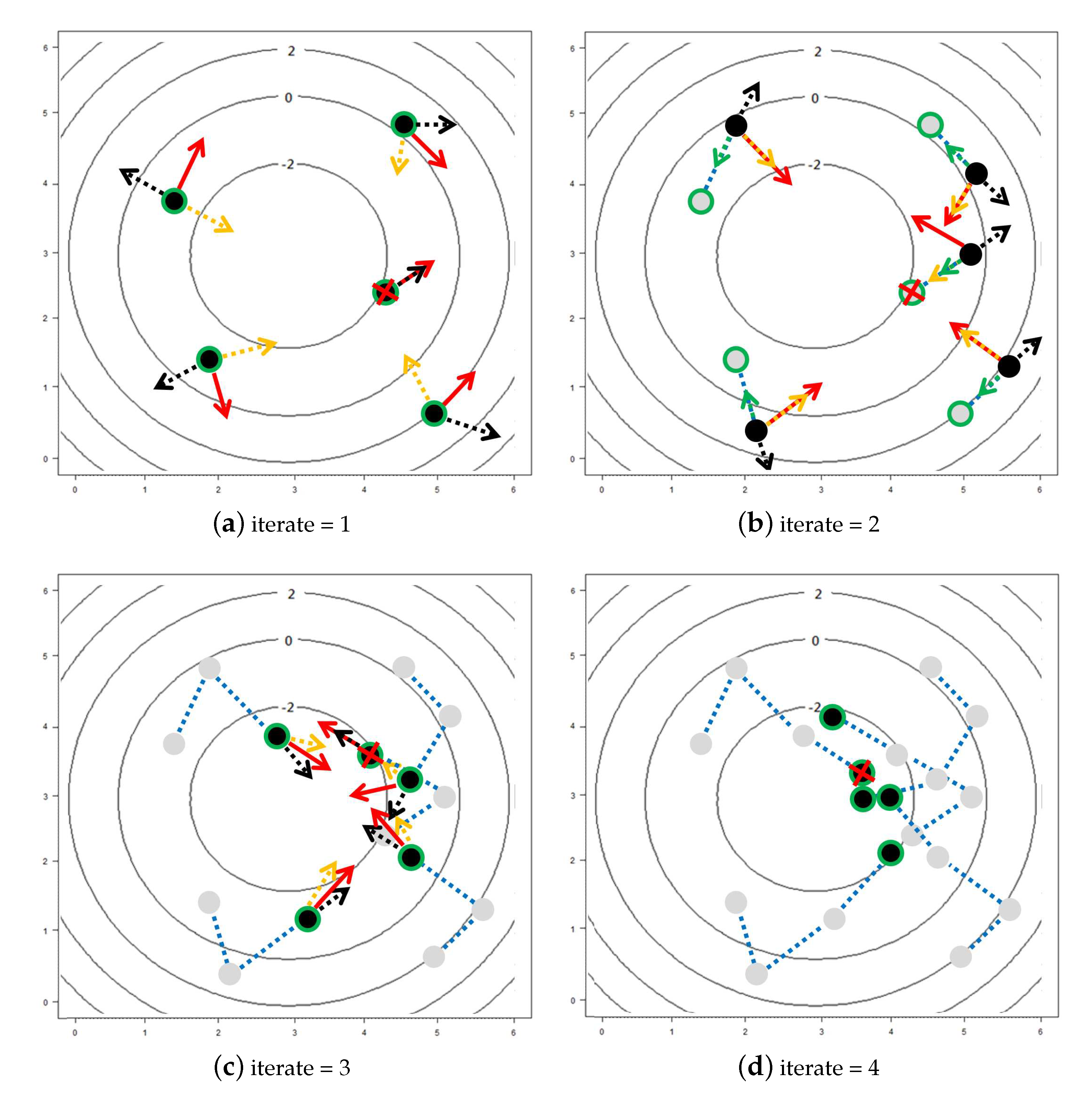
3. The Proposed Algorithm
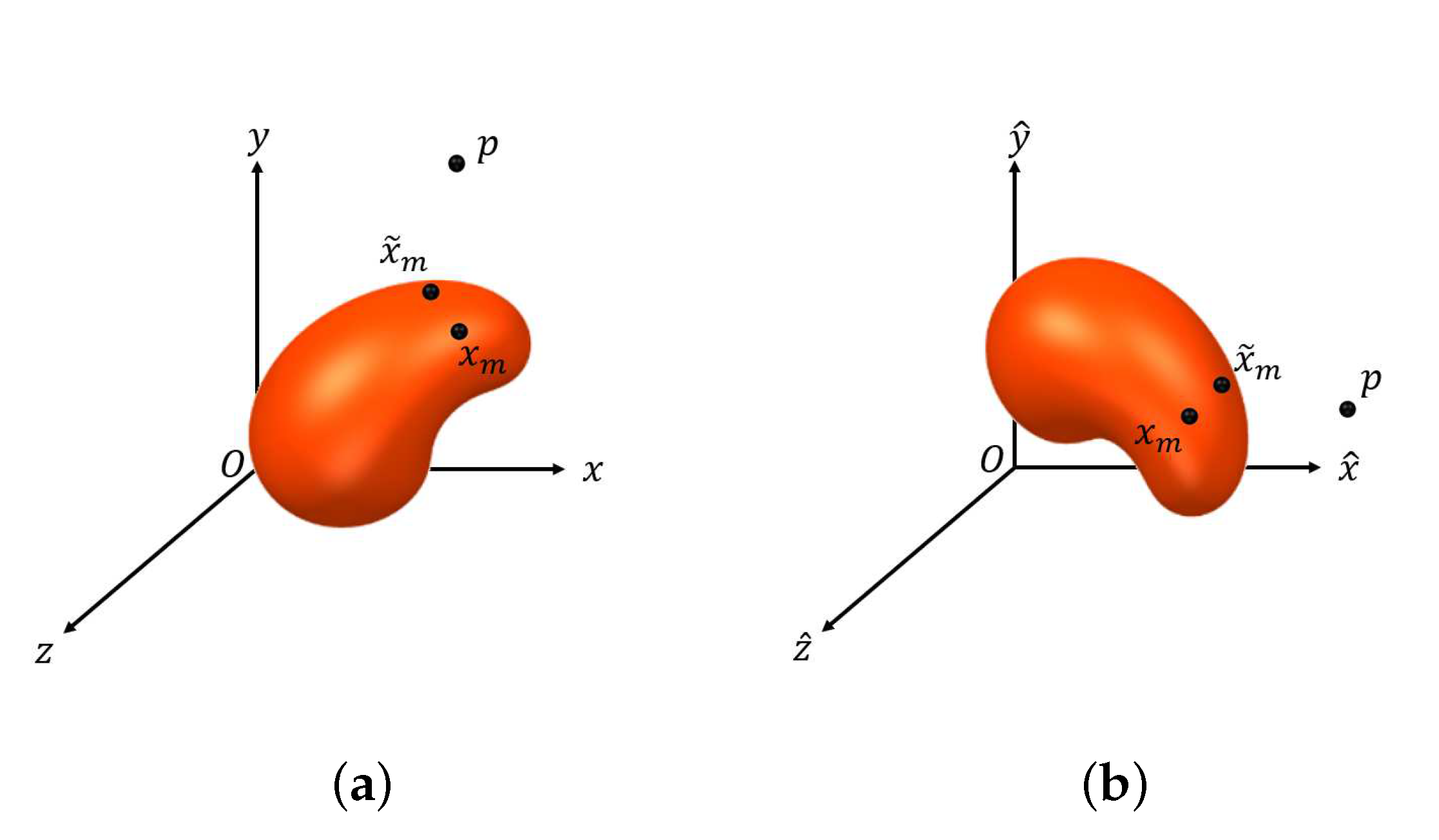
- Set an such that for all , we have , where is defined similarly to . Let denote the initial point for estimating and can be obtained by lettingwhere and denotes the set of boundary points of .
- Let be a predetermined tolerance, and set .
- (i)
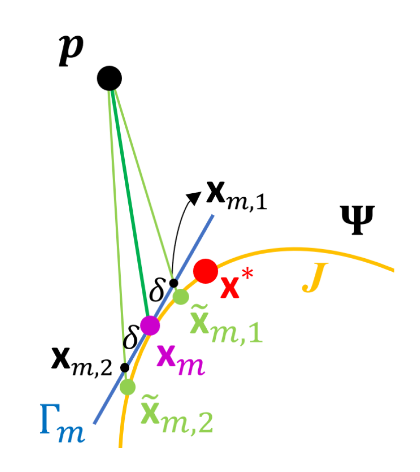
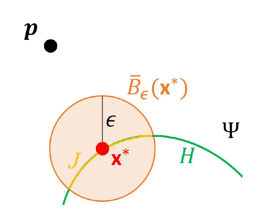
- Compute the tangent plane to at and denote it by . Let be a set of points on and , where is a predetermined positive constant.
- (ii)
- Let and as defined in (10), where , . Let
- (iii)
- Let , where , is the acute angle of two vectors, and , which denotes the normal vector to at . If , set and stop, where denotes the estimate of . Otherwise, set and repeat Steps (i) and (ii).
- C1.
- is continuously differentiable, denoted by .
- C2.
- For any fixed , , and , there exists a 2-dimensional neighborhood of , where with being a 2-dimensional open ball of radius centered at , such that and for any and , and for any , satisfies or .
4. Numerical Results
- Set 1
- Grayscale features (9 features): For each 2D-combined image, we compute the empirical density of the grayscale values, which are normalized into , and calculate 8 probabilities between two adjacent percentiles in to represent the ratios of areas having different magnitudes of uptakes. In addition, we also compute the ratios of average uptake values near striatum to the average uptake values of the background.
- Set 2
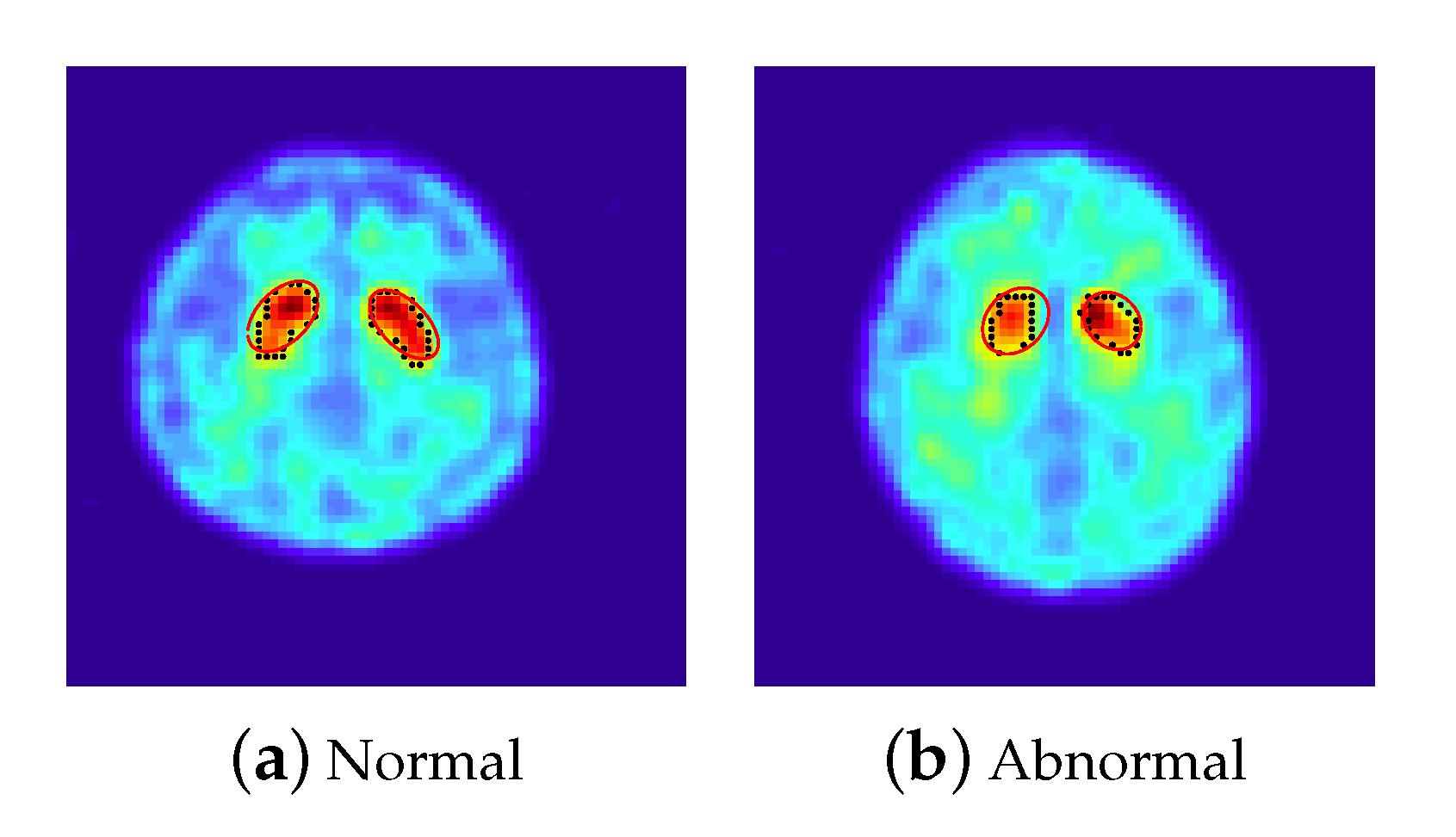
- The features extracted from the ellipse equations (12 features): We employed the PSO-FS algorithm to approximate the shape of striatum for each 2D-combined image by the criterion defined in (3), where 100 particles are randomly set centered on an initial estimator of . Figure 2 presents approximated ellipses in red of a normal subject and a subject with PD, which reveal that the PSO-FS algorithm is capable of obtaining satisfactory ellipses to approximate the shapes of uptakes.
- Set 3
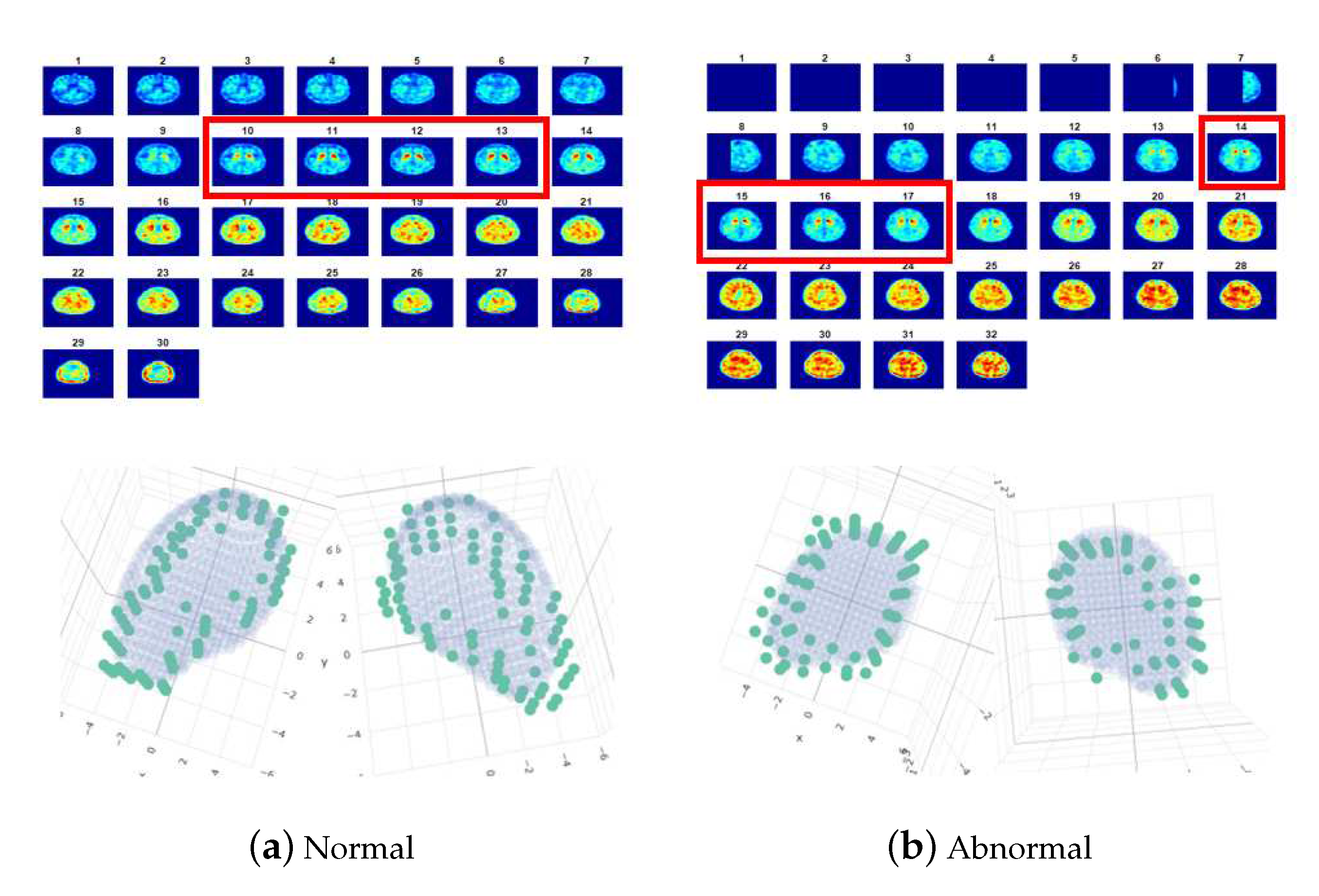
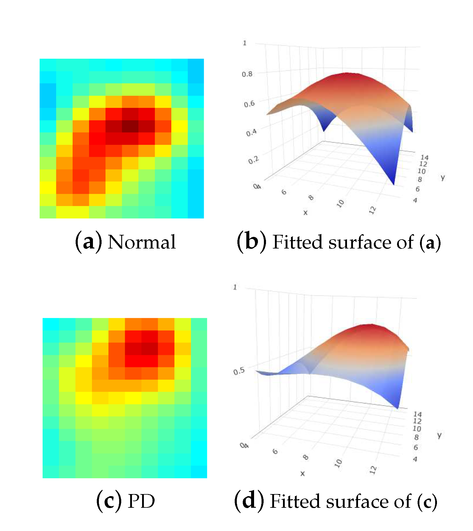
- The features extracted from the cashew-shaped equations (22 features): The procedure for fitting a 3D structure is similar to the above 2D shape fitting process. Figure 7 presents the sequences of 2D images in the upper panel and the corresponding cashew-shaped surfaces in 3D space in the lower panel of a normal subject and a subject with PD, where the 2D images in the red rectangles are recommended by the physicians and are used to construct the cashew-shaped surfaces. The fitting results shown in Figure 7 display that the PSO-FS algorithm is capable of obtaining satisfactory cashew-shaped equations to approximate the shapes of uptakes.
- Set 4
- The union of Sets 1 and 2.
- Set 5
- The union of Sets 1, 2, and 3.
- Set 6
- We randomly split the data into training and test sets with the proportions of 80% and 20%, respectively, under a stratified sampling scheme, where the proportions of normal, nearly normal, potentially abnormal, and abnormal subjects in the training and test sets are the same.
- In the training set, we conduct a stratified 5-fold CV framework on each of the SVM, NB, RF, XGB, LR, and LDA classifiers by R-packages svm(), naiveBayes(), randomForest(), xgboost(), glm(), and lda(), respectively. The tuning parameters in each of the SVM, RF, and XGB methods are determined by computing the validation accuracies under several settings of tuning parameters and selecting the one with the highest validation accuracy. For each of the SVM, RF, and XGB classifiers, we set 5 candidates for each tuning parameters centered at the default values of the corresponding R packages. Therefore, we have 6 candidate classifiers, where each of them has the best 5-fold CV performances for the training data.
- Let the classifier with the best 5-fold CV accuracy from the 6 candidates be our final selection. Learn this classifier again with all the training data and use it to compute the classification performances of the test data.
- Repeat the above 3 steps 100 times. Compute the mean and standard deviation (SD) of accuracy (ACC), sensitivity (SEN), specificity (SPE), and GM under the 5-fold CV framework of the 6 classifiers for training data, and compute the mean, SD, and 95% confidence interval (CI) of the 4 measurements for test data based on the results of the 100 rounds.
5. Discussion
- For a specific ROI, the proposed method needs to select a suitable family of mathematical representation, like the ellipse and cashew-shaped equations for identifying PD in 2D and 3D spaces, respectively. However, we may not have enough understanding or knowledge to derive useful features directly from a mathematical representation of any shape of the ROI, like the cashew-shaped equation used in this study. Therefore, we just adopt the coefficients of the shape equation as features for classification. Although these coefficients can represent the shape of the ROI, it may not be the most effective way for a suitable classifier to learn. More studies are needed to dig more insights for this issue.
- This study and [8] both adopted the family of ellipse equations to portray the ROI observed from an 2D-combined image for PD identification. However, the ROI for normal subjects should be comma-shaped, which is not an ellipse. Due to the reason that we know ellipses better than comma-shaped equations, the family of ellipse equations is selected to approximate the ROI. This selection, of course, has systematic biases (or called model risk), which might reduce the classification performance.
- In the proposed PSO-FS algorithm, we need to compute the distance of each boundary point of the ROI to a given shape equation in each PSO iteration. This procedure is computationally expensive, especially when training a classifier with a huge number of boundary points. A more efficiently computing way should be developed in the future.
Author Contributions
Funding
Conflicts of Interest
Appendix A. Derivation of the Cashew-Shaped Equation (5) Satisfying C2

- 1.
- G is continuous on , .
- 2.
- If and , there exists another point such that .

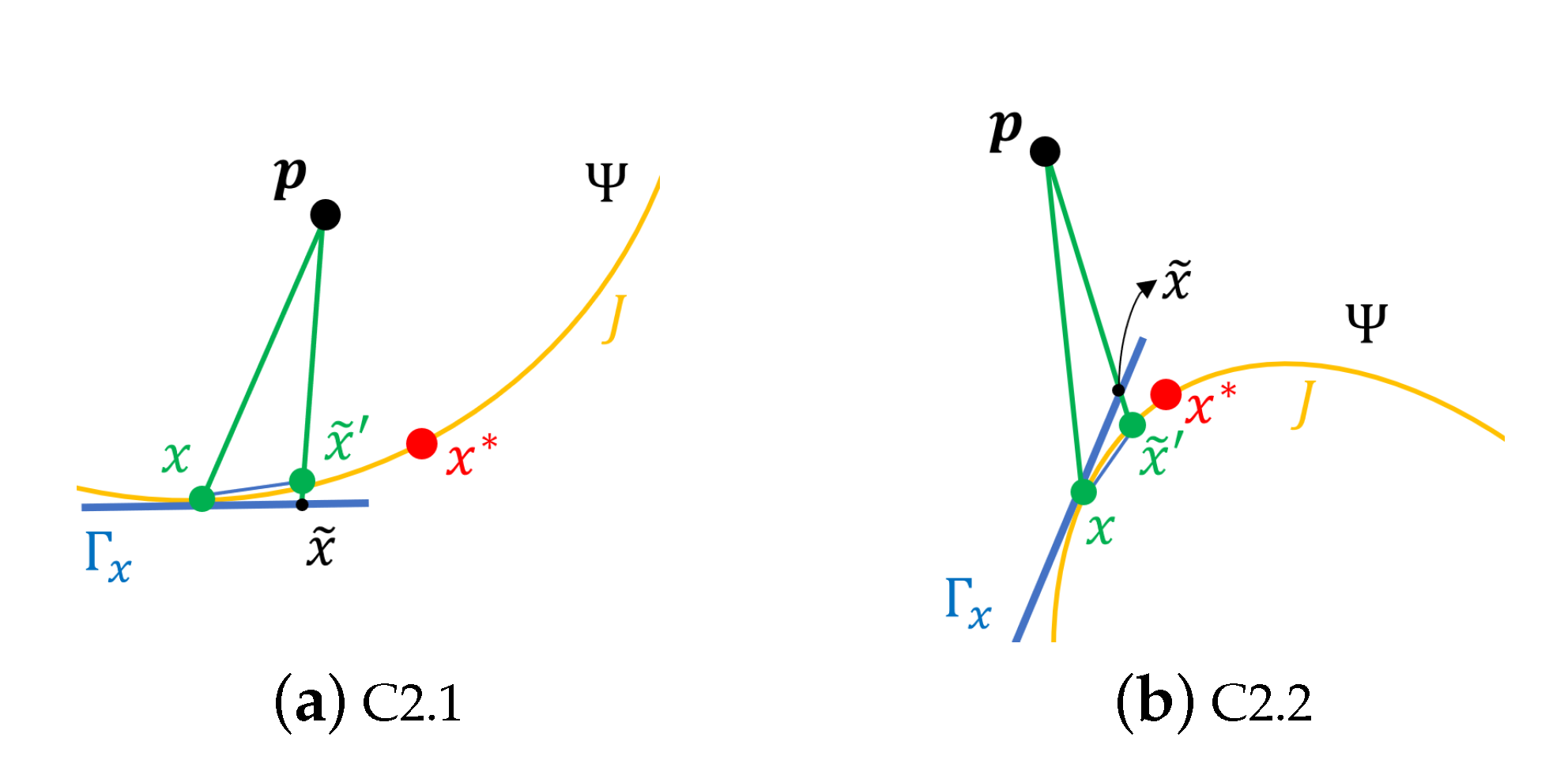
- C2.1
- , for ;
- C2.2
- , for .
References
- Prashanth, R.; Roy, S.D.; Mandal, P.K.; Ghosh, S. Automatic classification and prediction models for early Parkinson’s disease diagnosis from SPECT imaging. Expert Syst. Appl. 2014, 41, 3333–3342. [Google Scholar] [CrossRef]
- Taylor, J.C.; Fenner, J.W. Comparison of machine learning and semi-quantification algorithms for (I123) FP-CIT classification: The beginning of the end for semi-quantification? EJNMMI Phys. 2017, 4, 29. [Google Scholar] [CrossRef] [PubMed] [Green Version]
- Oliveira, F.P.; Faria, D.B.; Costa, D.C.; Castelo-Branco, M.; Tavares, J.M.R. Extraction, selection and comparison of features for an effective automated computer-aided diagnosis of Parkinson’s disease based on [123 I] FP-CIT SPECT images. Eur. J. Nucl. Med. Mol. Imaging 2018, 45, 1052–1062. [Google Scholar] [CrossRef] [Green Version]
- Nicastro, N.; Wegrzyk, J.; Preti, M.G.; Fleury, V.; Van de Ville, D.; Garibotto, V.; Burkhard, P.R. Classification of degenerative parkinsonism subtypes by support-vector-machine analysis and striatal 123 I-FP-CIT indices. J. Neurol. 2019, 266, 1771–1781. [Google Scholar] [CrossRef] [PubMed] [Green Version]
- Iwabuchi, Y.; Nakahara, T.; Kameyama, M.; Yamada, Y.; Hashimoto, M.; Matsusaka, Y.; Osada, T.; Ito, D.; Tabuchi, H.; Jinzaki, M. Impact of a combination of quantitative indices representing uptake intensity, shape, and asymmetry in DAT SPECT using machine learning: Comparison of different volume of interest settings. EJNMMI Res. 2019, 9, 7. [Google Scholar] [CrossRef] [PubMed]
- Ziegler, D.A.; Wonderlick, J.S.; Ashourian, P.; Hansen, L.A.; Young, J.C.; Murphy, A.J.; Koppuzha, C.K.; Growdon, J.H.; Corkin, S. Substantia nigra volume loss before basal forebrain degeneration in early Parkinson disease. JAMA Neurol. 2013, 70, 241–247. [Google Scholar] [CrossRef] [PubMed] [Green Version]
- Palumbo, B.; Fravolini, M.L.; Buresta, T.; Pompili, F.; Forini, N.; Nigro, P.; Calabresi, P.; Tambasco, N. Diagnostic accuracy of Parkinson disease by support vector machine (SVM) analysis of 123I-FP-CIT brain SPECT data: Implications of putaminal findings and age. Medicine 2014, 93, e228. [Google Scholar] [CrossRef]
- Prashanth, R.; Roy, S.D.; Mandal, P.K.; Ghosh, S. High-accuracy classification of Parkinson’s disease through shape analysis and surface fitting in 123I-Ioflupane SPECT imaging. IEEE J. Biomed. Health Inform. 2016, 21, 794–802. [Google Scholar] [CrossRef] [Green Version]
- Hsu, S.Y.; Lin, H.C.; Chen, T.B.; Du, W.C.; Hsu, Y.H.; Wu, Y.C.; Tu, P.W.; Huang, Y.H.; Chen, H.Y. Feasible classified models for Parkinson disease from 99mTc-TRODAT-1 SPECT imaging. Sensors 2019, 19, 1740. [Google Scholar] [CrossRef] [Green Version]
- Cheng, Z.; Zhang, J.; He, N.; Li, Y.; Wen, Y.; Xu, H.; Tang, R.; Jin, Z.; Haacke, M.; Yan, F.; et al. Radiomic features of the Nigrosome-1 region of the substantia nigra: Using quantitative susceptibility mapping to assist the diagnosis of idiopathic Parkinson’s disease. Front. Aging Neurosci. 2019, 11, 167. [Google Scholar] [CrossRef] [Green Version]
- Xu, R.; Hu, X.; Jiang, X.; Zhang, Y.; Wang, J.; Zeng, X. Longitudinal volume changes of hippocampal subfields and cognitive decline in Parkinson’s disease. Quant. Imaging Med. Surg. 2020, 10, 220–232. [Google Scholar] [CrossRef] [PubMed]
- Kalia, L.V.; Lang, A.E. Parkinson’s disease. Lancet 2015, 386, 896–912. [Google Scholar] [CrossRef]
- Hayes, M.T. Parkinson’s disease and Parkinsonism. Am. J. Med. 2019, 132, 802–807. [Google Scholar] [CrossRef] [PubMed]
- Kung, H.F.; Kung, M.P.; Wey, S.P.; Lin, K.J.; Yen, T.C. Clinical acceptance of a molecular imaging agent: A long march with [99mTc] TRODAT. Nucl. Med. Biol. 2007, 34, 787–789. [Google Scholar] [CrossRef]
- Bajaj, N.; Hauser, R.A.; Grachev, I.D. Clinical utility of dopamine transporter single photon emission CT (DaT-SPECT) with (123I) ioflupane in diagnosis of parkinsonian syndromes. J. Neurol. Neurosurg. Psychiatry 2013, 84, 1288–1295. [Google Scholar] [CrossRef] [Green Version]
- Törn, A.; Žilinskas, A. Global Optimization; Springer: Berlin, Germany, 1989. [Google Scholar]
- Eberhart, R.; Kennedy, J. Particle swarm optimization. In Proceedings of the IEEE International Conference on Neural Networks, Perth, WA, Australia, 27 November–1 December 1995; Volume 4, pp. 1942–1948. [Google Scholar]
- Delgarm, N.; Sajadi, B.; Kowsary, F.; Delgarm, S. Multi-objective optimization of the building energy performance: A simulation-based approach by means of particle swarm optimization (PSO). Appl. Energy 2016, 170, 293–303. [Google Scholar] [CrossRef]
- Mistry, K.; Zhang, L.; Neoh, S.C.; Lim, C.P.; Fielding, B. A micro-GA embedded PSO feature selection approach to intelligent facial emotion recognition. IEEE Trans. Cybern. 2016, 47, 1496–1509. [Google Scholar] [CrossRef] [PubMed] [Green Version]
- Hasanipanah, M.; Naderi, R.; Kashir, J.; Noorani, S.A.; Qaleh, A.Z.A. Prediction of blast-produced ground vibration using particle swarm optimization. Eng. Comput. 2017, 33, 173–179. [Google Scholar] [CrossRef]
- Kumar, A.; Pant, S.; Ram, M.; Singh, S.B. On solving complex reliability optimization problem using multi-objective particle swarm optimization. In Mathematics Applied to Engineering; Academic Press: London, UK, 2017; pp. 115–131. [Google Scholar]
- Morera, D.M.; Sarlabous, J.E. On the distance from a point to a quadric surface. Investig. Oper. 2003, 24, 153–161. [Google Scholar]
- Rovini, E.; Maremmani, C.; Moschetti, A.; Esposito, D.; Cavallo, F. Comparative motor pre-clinical assessment in Parkinson’s disease using supervised machine learning approaches. Ann Biomed. Eng. 2018, 46, 2057–2068. [Google Scholar] [CrossRef]
- Chen, T.; Guestrin, C. Xgboost: A scalable tree boosting system. In Proceedings of the 22nd ACM SIGKDD International Conference on Knowledge Discovery and Data Mining, San Francisco, CA, USA, 13–17 August 2016; pp. 785–794. [Google Scholar]
- Huang, S.F.; Lu, H.P. Classification of temporal data using dynamic time warping andcompressed learning. Biomed. Signal Process. Control 2020, 57, 101781. [Google Scholar] [CrossRef]
- Dolz, J.; Desrosiers, C.; Ayed, I.B. 3D fully convolutional networks for subcortical segmentation in MRI: A large-scale study. NeuroImage 2018, 170, 456–470. [Google Scholar] [CrossRef] [PubMed] [Green Version]
- Carr, J.C.; Fright, W.R.; Beatson, R.K. Surface interpolation with radial basis functions for medical imaging. IEEE Trans. Med. Imaging 1997, 16, 96–107. [Google Scholar] [CrossRef] [PubMed]
- Pu, J.; Zheng, B.; Leader, J.K.; Fuhrman, C.; Knollmann, F.; Klym, A.; Gur, D. Pulmonary lobe segmentation in CT examinations using implicit surface fitting. IEEE Trans. Med. Imaging 2009, 28, 1986–1996. [Google Scholar] [PubMed] [Green Version]
- Huang, A.; Summers, R.M.; Hara, A.K. Surface curvature estimation for automatic colonic polyp detection. In Proceedings of the Medical Imaging 2005: Physiology, Function, and Structure from Medical Images, San Diego, CA, USA, 12–17 February 2005; pp. 393–402. [Google Scholar]
- Hu, X.; Eberhart, R. Solving constrained nonlinear optimization problems with particle swarm optimization. In Proceedings of the Sixth World Multiconference on Systemics, Cybernetics and Informatics, Orlando, FL, USA, 14–18 July 2002; Volume 5, pp. 203–206. [Google Scholar]
- Robinson, J.; Rahmat-Samii, Y. Particle swarm optimization in electromagnetics. IEEE Trans. Antennas Propag. 2004, 52, 397–407. [Google Scholar] [CrossRef]
- Sumardi, M.S.; Riyadi, M.A. Particle swarm optimization (PSO)-based self tuning proportional integral derivative (PID) for bearing navigation control system on quadcopter. In Proceedings of the 4th International Conference on Information Technology, Computer, and Electrical Engineering, Semarang, Indonesia, 18–19 October 2017; pp. 181–186. [Google Scholar]
- Kuncheva, L.I.; Arnaiz-Gonzalez, A.; Diez-Pastor, J.F.; Gunn, I.A. Instance selection improves geometric mean accuracy: A study on imbalanced data classification. Prog. Artif. Intell. 2019, 8, 215–228. [Google Scholar] [CrossRef] [Green Version]


| Normal | Abnormal | |||||||
|---|---|---|---|---|---|---|---|---|
| 2D | 3D | 2D | 3D | |||||
| L | R | L | R | L | R | L | R | |
| mean | 0.55 | 0.69 | 33.75 | 42.22 | 0.40 | 0.40 | 34.28 | 30.52 |
| SD | 0.01 | 0.14 | 1.43 | 3.81 | 0.01 | 0.04 | 0.97 | 0.95 |
| Classifier | ||||||||
|---|---|---|---|---|---|---|---|---|
| Measure | Set | SVM | NB | RF | XGB | LR | LDA | |
| ACC | 1 | AVE | 0.865 | 0.753 | 0.866 | 0.836 | 0.842 | 0.848 |
| SD | 0.008 | 0.008 | 0.009 | 0.013 | 0.009 | 0.008 | ||
| 2 | AVE | 0.798 | 0.760 | 0.793 | 0.747 | 0.789 | 0.776 | |
| SD | 0.008 | 0.007 | 0.010 | 0.015 | 0.010 | 0.010 | ||
| 3 | AVE | 0.798 | 0.805 | 0.826 | 0.788 | 0.824 | 0.819 | |
| SD | 0.012 | 0.009 | 0.010 | 0.016 | 0.010 | 0.009 | ||
| 4 | AVE | 0.873 | 0.788 | 0.880 | 0.845 | 0.854 | 0.862 | |
| SD | 0.007 | 0.008 | 0.007 | 0.013 | 0.009 | 0.008 | ||
| 5 | AVE | 0.824 | 0.824 | 0.880 | 0.835 | 0.855 | 0.859 | |
| SD | 0.010 | 0.008 | 0.007 | 0.012 | 0.011 | 0.009 | ||
| 6 | AVE | 0.619 | 0.620 | 0.865 | 0.830 | 0.849 | 0.857 | |
| SD | 0.011 | 0.012 | 0.009 | 0.014 | 0.004 | 0.009 | ||
| SEN | 1 | AVE | 0.823 | 0.564 | 0.846 | 0.825 | 0.819 | 0.765 |
| SD | 0.013 | 0.014 | 0.011 | 0.018 | 0.012 | 0.015 | ||
| 2 | AVE | 0.760 | 0.642 | 0.785 | 0.734 | 0.772 | 0.700 | |
| SD | 0.015 | 0.011 | 0.013 | 0.018 | 0.013 | 0.016 | ||
| 3 | AVE | 0.715 | 0.706 | 0.775 | 0.760 | 0.799 | 0.771 | |
| SD | 0.026 | 0.017 | 0.014 | 0.021 | 0.013 | 0.013 | ||
| 4 | AVE | 0.845 | 0.656 | 0.870 | 0.828 | 0.836 | 0.802 | |
| SD | 0.010 | 0.013 | 0.008 | 0.017 | 0.013 | 0.011 | ||
| 5 | AVE | 0.766 | 0.733 | 0.874 | 0.813 | 0.843 | 0.818 | |
| SD | 0.017 | 0.012 | 0.009 | 0.016 | 0.013 | 0.012 | ||
| 6 | AVE | 0.975 | 0.286 | 0.852 | 0.815 | 0.846 | 0.812 | |
| SD | 0.006 | 0.024 | 0.010 | 0.017 | 0.007 | 0.013 | ||
| SPE | 1 | AVE | 0.911 | 0.963 | 0.888 | 0.848 | 0.867 | 0.939 |
| SD | 0.014 | 0.005 | 0.012 | 0.019 | 0.013 | 0.010 | ||
| 2 | AVE | 0.841 | 0.891 | 0.802 | 0.761 | 0.808 | 0.861 | |
| SD | 0.015 | 0.009 | 0.016 | 0.020 | 0.013 | 0.013 | ||
| 3 | AVE | 0.891 | 0.915 | 0.882 | 0.818 | 0.853 | 0.873 | |
| SD | 0.020 | 0.011 | 0.012 | 0.019 | 0.014 | 0.012 | ||
| 4 | AVE | 0.903 | 0.935 | 0.890 | 0.864 | 0.873 | 0.928 | |
| SD | 0.011 | 0.006 | 0.011 | 0.019 | 0.013 | 0.011 | ||
| 5 | AVE | 0.888 | 0.925 | 0.888 | 0.858 | 0.869 | 0.904 | |
| SD | 0.016 | 0.009 | 0.009 | 0.018 | 0.014 | 0.011 | ||
| 6 | AVE | 0.224 | 0.990 | 0.879 | 0.847 | 0.851 | 0.907 | |
| SD | 0.022 | 0.004 | 0.014 | 0.021 | 0.006 | 0.013 | ||
| GM | 1 | AVE | 0.866 | 0.737 | 0.867 | 0.837 | 0.843 | 0.848 |
| SD | 0.008 | 0.010 | 0.009 | 0.013 | 0.009 | 0.008 | ||
| 2 | AVE | 0.799 | 0.756 | 0.793 | 0.747 | 0.790 | 0.776 | |
| SD | 0.008 | 0.008 | 0.010 | 0.015 | 0.010 | 0.010 | ||
| 3 | AVE | 0.798 | 0.804 | 0.827 | 0.788 | 0.825 | 0.820 | |
| SD | 0.012 | 0.010 | 0.010 | 0.016 | 0.010 | 0.009 | ||
| 4 | AVE | 0.874 | 0.783 | 0.880 | 0.845 | 0.854 | 0.863 | |
| SD | 0.007 | 0.008 | 0.007 | 0.013 | 0.009 | 0.008 | ||
| 5 | AVE | 0.825 | 0.824 | 0.881 | 0.835 | 0.856 | 0.860 | |
| SD | 0.010 | 0.008 | 0.007 | 0.012 | 0.011 | 0.009 | ||
| 6 | AVE | 0.467 | 0.531 | 0.865 | 0.831 | 0.849 | 0.858 | |
| SD | 0.023 | 0.022 | 0.009 | 0.014 | 0.004 | 0.009 | ||
| Measure | # Times | ||||||||||
|---|---|---|---|---|---|---|---|---|---|---|---|
| Set | ACC | SEN | SPE | GM | |||||||
| 1 | AVE | 0.858 | 0.822 | 0.898 | 0.859 | 45 | 0 | 54 | 0 | 1 | 0 |
| SD | 0.024 | 0.042 | 0.036 | 0.024 | |||||||
| 95%CI | (0.81,0.91) | (0.74,0.91) | (0.83,0.97) | (0.81,0.91) | |||||||
| 2 | AVE | 0.792 | 0.759 | 0.828 | 0.792 | 60 | 0 | 23 | 0 | 17 | 0 |
| SD | 0.024 | 0.045 | 0.047 | 0.024 | |||||||
| 95%CI | (0.74,0.84) | (0.67,0.85) | (0.73,0.92) | (0.74,0.84) | |||||||
| 3 | AVE | 0.825 | 0.788 | 0.866 | 0.825 | 0 | 0 | 54 | 0 | 41 | 5 |
| SD | 0.028 | 0.049 | 0.045 | 0.028 | |||||||
| 95%CI | (0.77,0.88) | (0.69,0.89) | (0.78,0.96) | (0.77,0.88) | |||||||
| 4 | AVE | 0.873 | 0.855 | 0.892 | 0.873 | 18 | 0 | 80 | 0 | 0 | 2 |
| SD | 0.023 | 0.039 | 0.038 | 0.024 | |||||||
| 95%CI | (0.83,0.92) | (0.78,0.93) | (0.82,0.97) | (0.83,0.92) | |||||||
| 5 | AVE | 0.880 | 0.872 | 0.888 | 0.880 | 0 | 0 | 99 | 0 | 0 | 1 |
| SD | 0.023 | 0.031 | 0.038 | 0.023 | |||||||
| 95%CI | (0.83,0.93) | (0.81,0.93) | (0.81,0.96) | (0.83,0.93) | |||||||
| 6 | AVE | 0.858 | 0.839 | 0.878 | 0.858 | 0 | 0 | 78 | 0 | 3 | 19 |
| SD | 0.026 | 0.039 | 0.041 | 0.026 | |||||||
| 95%CI | (0.81,0.91) | (0.76,0.92) | (0.80,0.96) | (0.81,0.91) | |||||||
Publisher’s Note: MDPI stays neutral with regard to jurisdictional claims in published maps and institutional affiliations. |
© 2020 by the authors. Licensee MDPI, Basel, Switzerland. This article is an open access article distributed under the terms and conditions of the Creative Commons Attribution (CC BY) license (http://creativecommons.org/licenses/by/4.0/).
Share and Cite
Huang, S.-F.; Wen, Y.-H.; Chu, C.-H.; Hsu, C.-C. A Shape Approximation for Medical Imaging Data. Sensors 2020, 20, 5879. https://doi.org/10.3390/s20205879
Huang S-F, Wen Y-H, Chu C-H, Hsu C-C. A Shape Approximation for Medical Imaging Data. Sensors. 2020; 20(20):5879. https://doi.org/10.3390/s20205879
Chicago/Turabian StyleHuang, Shih-Feng, Yung-Hsuan Wen, Chi-Hsiang Chu, and Chien-Chin Hsu. 2020. "A Shape Approximation for Medical Imaging Data" Sensors 20, no. 20: 5879. https://doi.org/10.3390/s20205879
APA StyleHuang, S.-F., Wen, Y.-H., Chu, C.-H., & Hsu, C.-C. (2020). A Shape Approximation for Medical Imaging Data. Sensors, 20(20), 5879. https://doi.org/10.3390/s20205879