Introduction to Noise Radar and Its Waveforms


 , ,
, ,  and
and
Abstract
1. Introduction
- Hard, if not impossible, exploitation of the transmitted signals by an enemy party aimed to intercept, classify, identify (and possibly jam) the radar. The low probability of intercept, i.e., the reduced visibility of radar signals by ESM (electronic support measures) and ELINT (electronic intelligence) systems [4] is significantly enhanced by the random nature of NRT signals. The low probability of intercept and low probability of exploitation by a hostile counterpart will be analysed in more detail in a companion paper to be submitted on the counter-interception and counter-exploitation features of NRT.
- Limitation of the mutual interferences to/from many radars located in a crowded environment and operating in a limited frequency band. In fact, using NRT the interfered radar perceives and treats the interference as a kind of noise [5,6]. This feature will be more and more important in the developments of marine radars, due to their use of solid-state transmitters, having much greater “duty cycle” (longer pulses) than the legacy magnetron [7], as well as in automotive applications, [8] because of the more and increasing number of used automotive radars, causing a high spatial density of these particular radar sets.
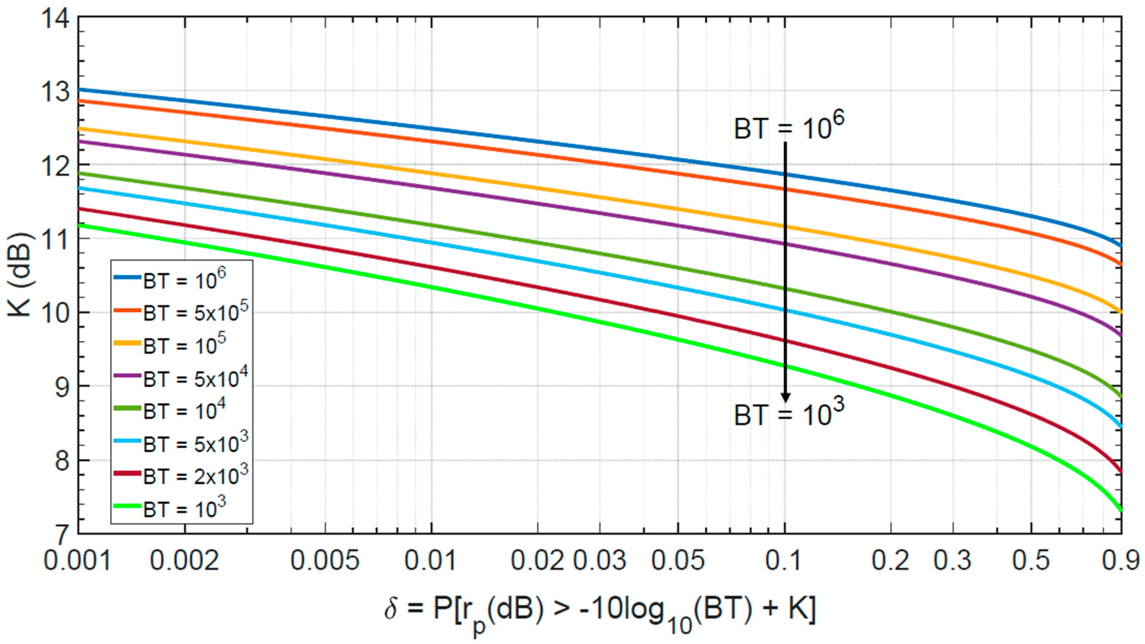
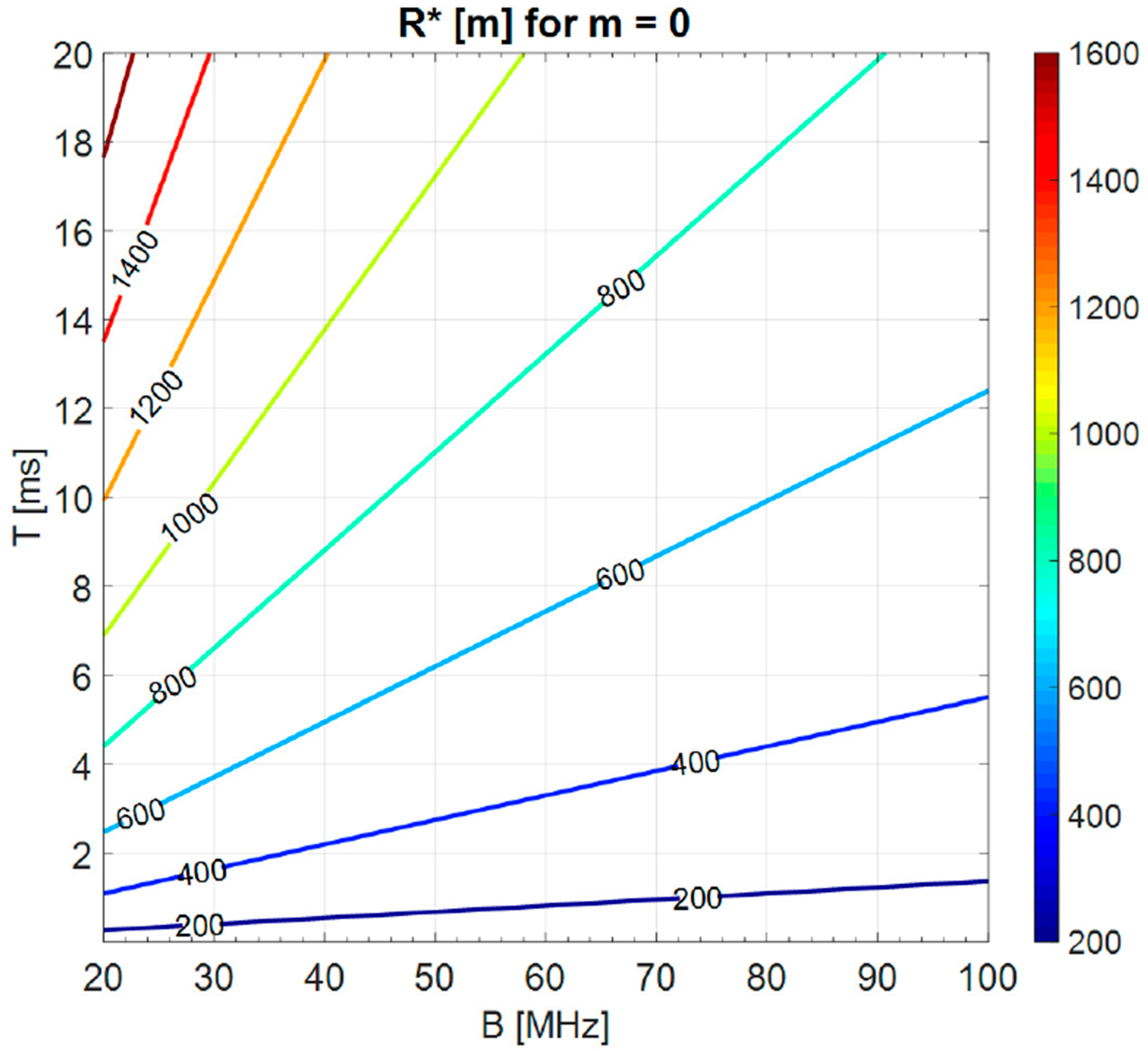
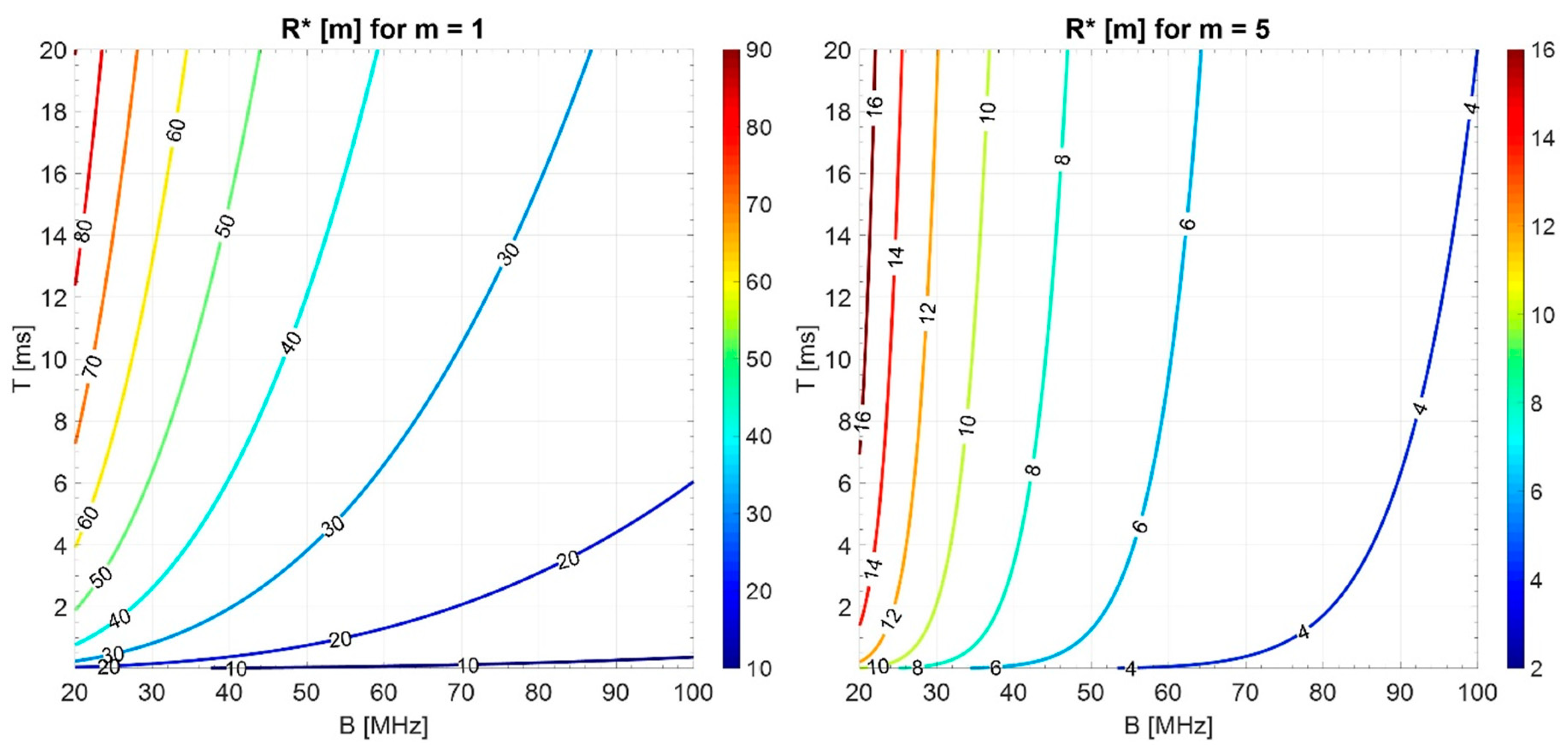
- Favourable shape of the “ambiguity function”. The ambiguity function [1,2] of a radar waveform defines its “selectivity” both in distance, i.e., in radar range (proportional to the time delay) and in radial velocity (proportional to the frequency shift due to the Doppler effect). The ambiguity function of a conceptual waveform made up by an infinitely long realization of “white noise” (i.e., with duration and bandwidth both going to infinity) tends to a Dirac’s “delta-shape” function with an ambiguity level going to zero. However, in all real applications both and are limited, and the peak side lobe ratio (PSLR) of the ambiguity function has a mean value close to the “processing gain” (hereafter,). Both bandwidth and duration are practically limited. The limitations on come from many factors, including the constraints on the usable portion of the electromagnetic spectrum [9]. Those on depend (i) on the dynamic behaviour (“decorrelation time”, ) of the radar cross section of most targets and (ii) on the dwell time, , and the pertaining type of radar processing. Echoes from moving targets (vehicles) have some typical decorrelation time (related to the signal fluctuation) of the rough order of hundreds of milliseconds. Doppler effect may pose a further limitation on the coherent signal integration time , imposed to be smaller than both and , and typically in the order of tens or hundreds of milliseconds. With an exemplary bandwidth of 50 MHz and an exemplary value of ms, the processing gain of a continuous-emission (CE) noise radar is of the order of one million. The resulting average PSLR is about 60 dB, which is acceptable in many radar applications, when the “fourth power of distance” term does not affect too much the needed dynamic range.
2. Noise Waveforms Properties
2.1. Deterministic Waveforms and Noise Waveforms
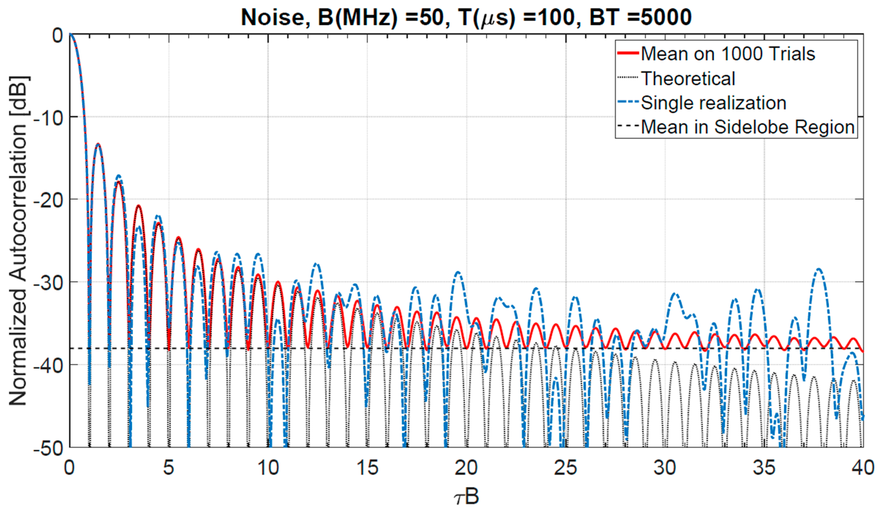
2.2. Statistical Properties of Autocorrelation Function, Sidelobes, and Power Spectrum
2.2.1. Noise Waveforms with Uniform Power Spectrum
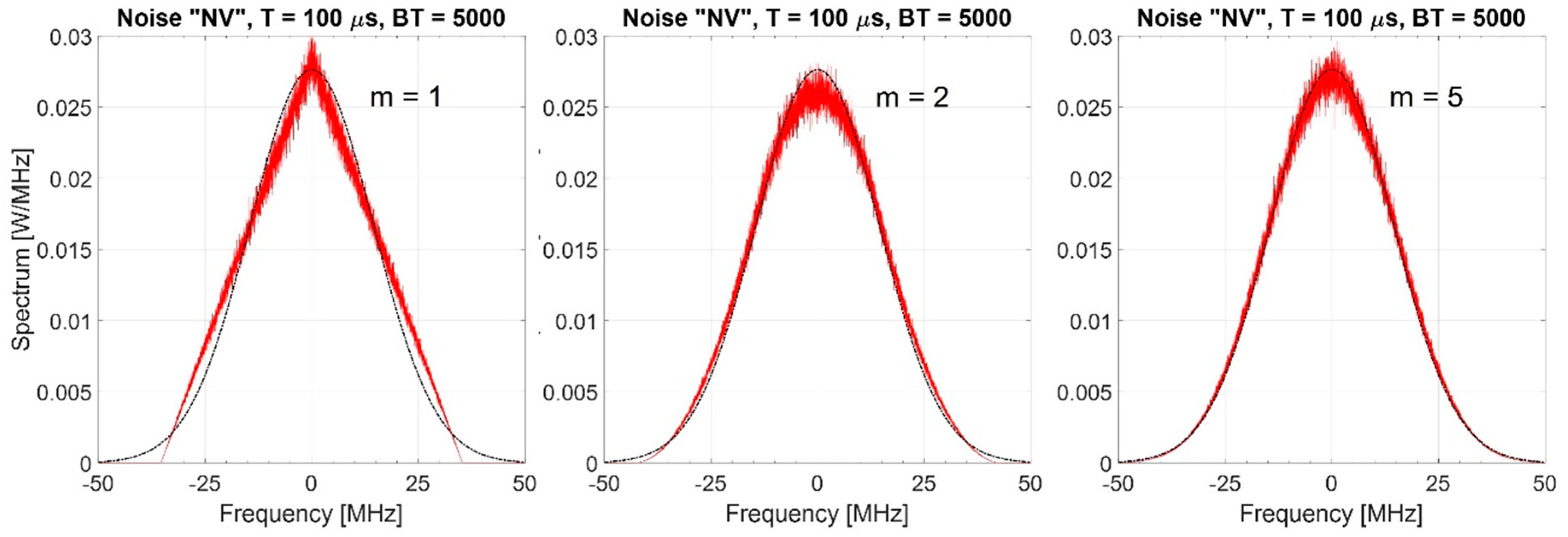
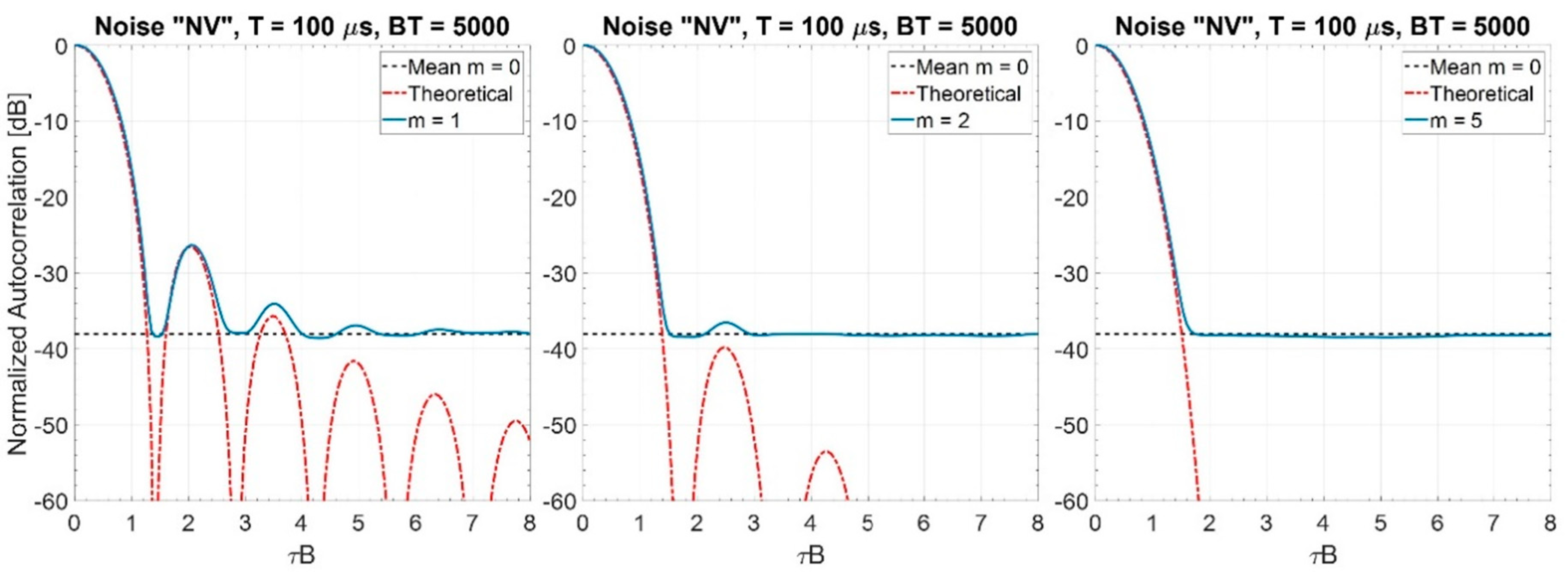
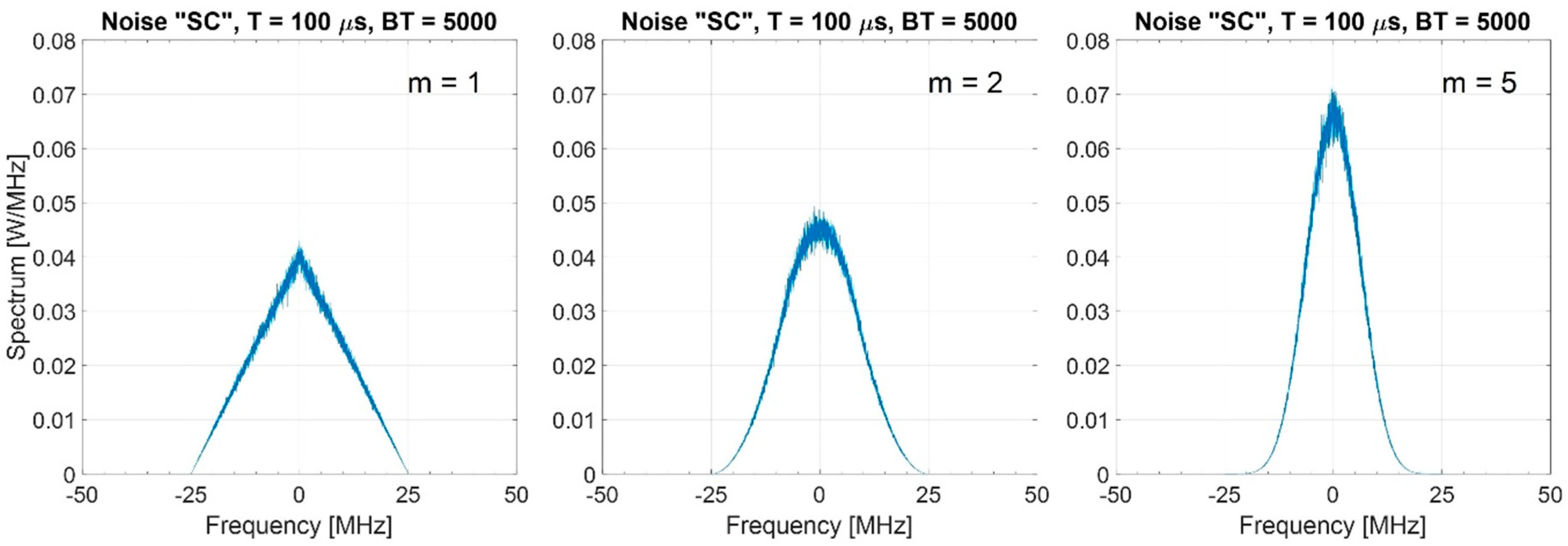
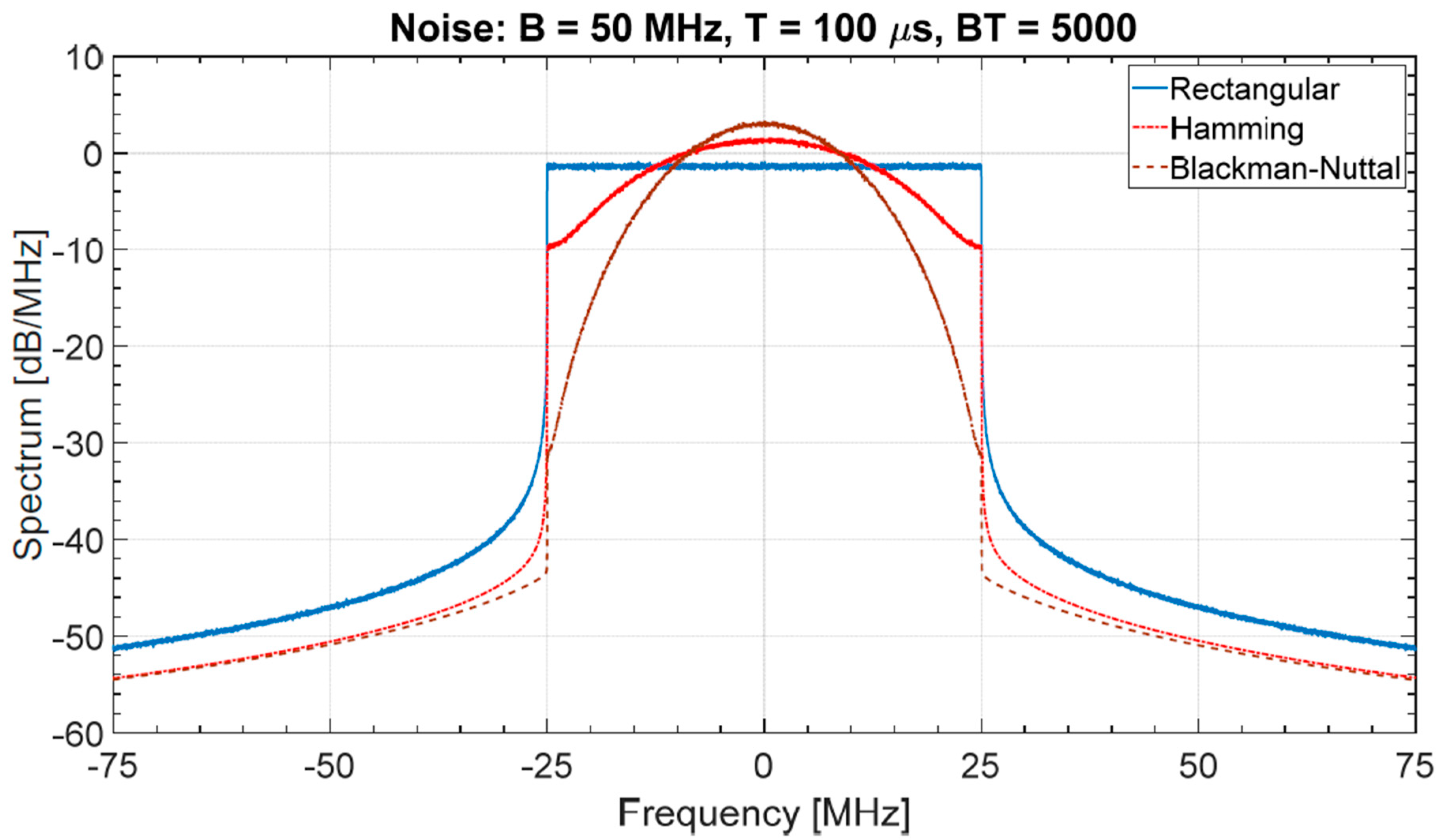
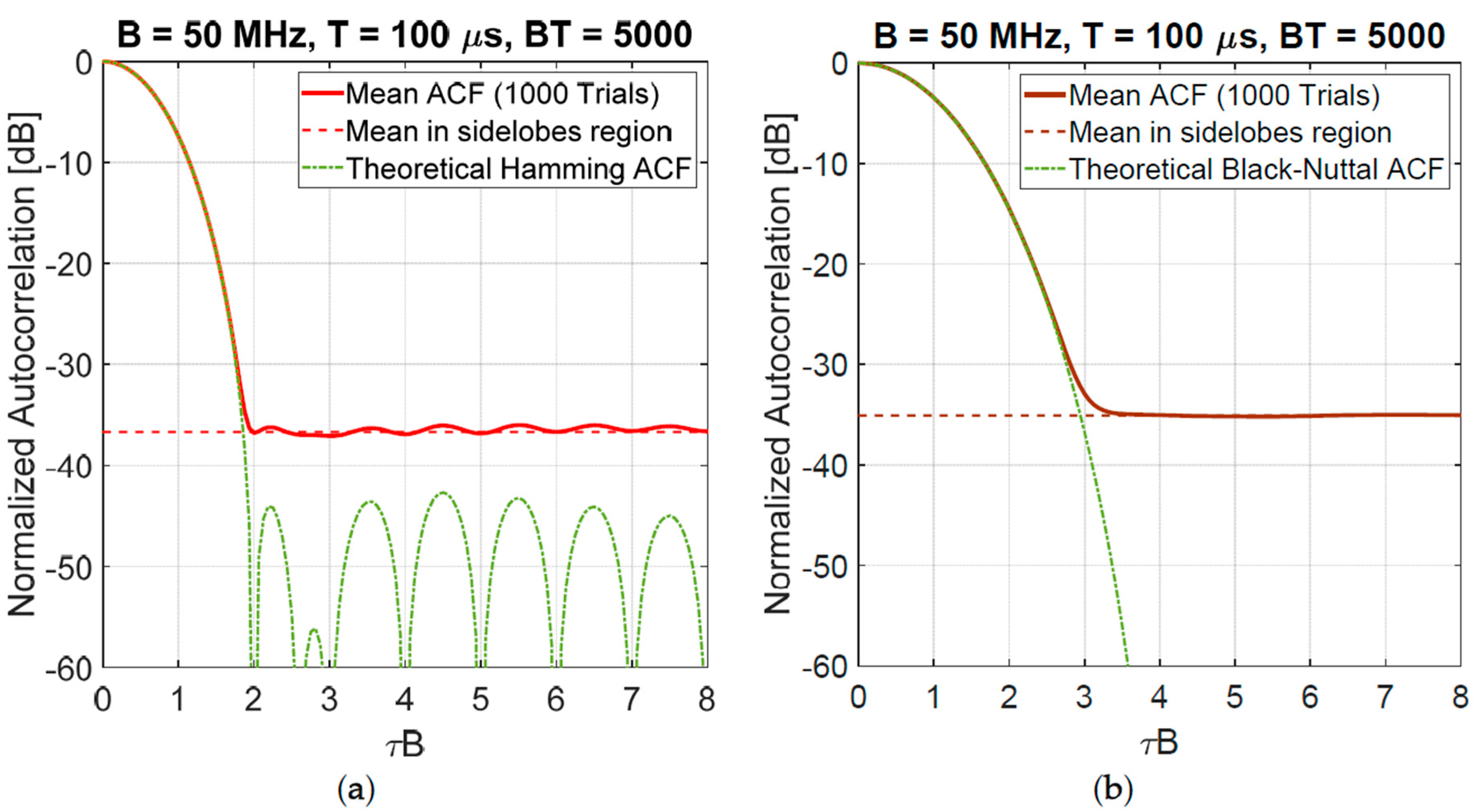
2.2.2. Noise Waveforms with “Shaped” Power Spectrum
- (i)
- the main lobe width is ; and
- (ii)
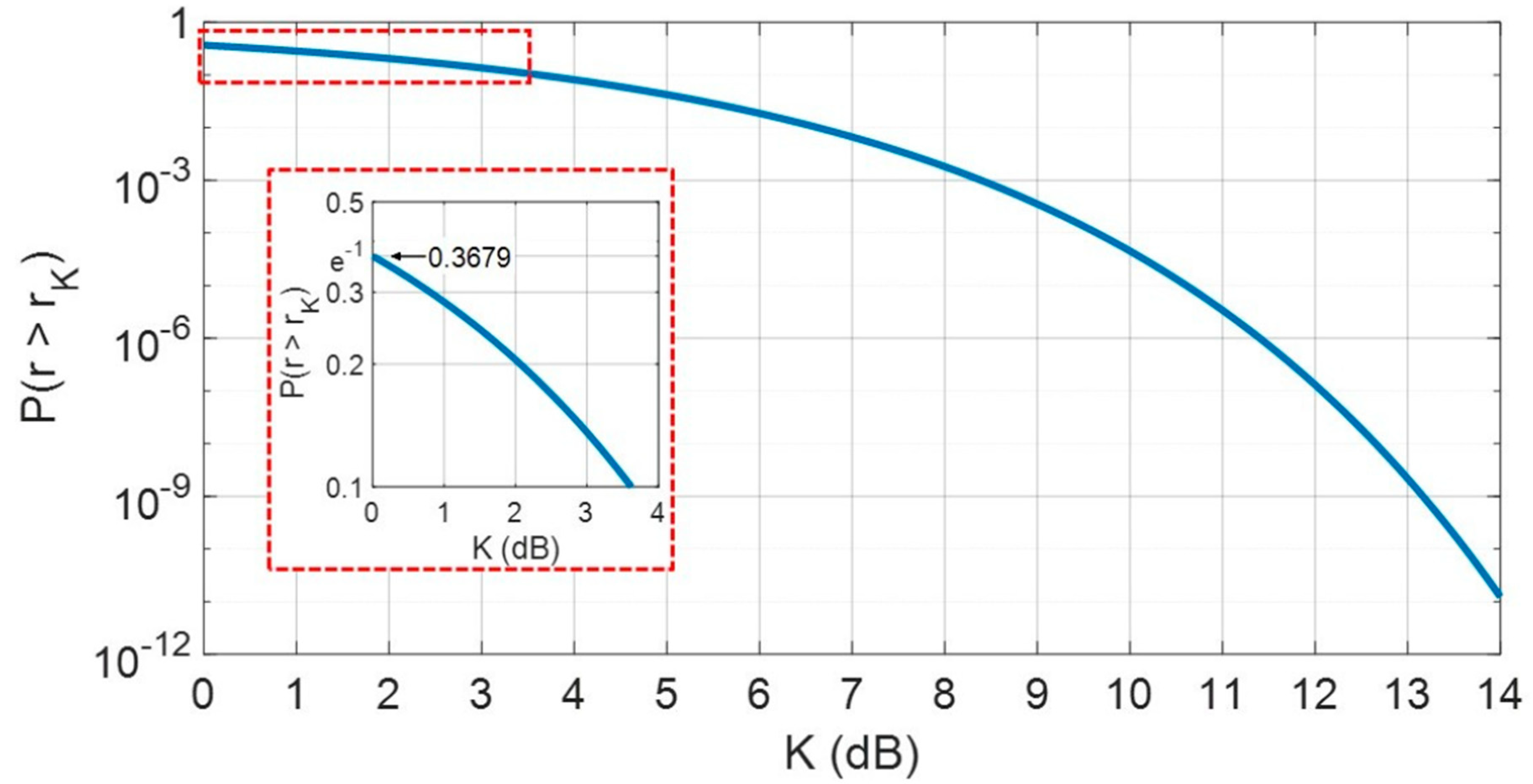
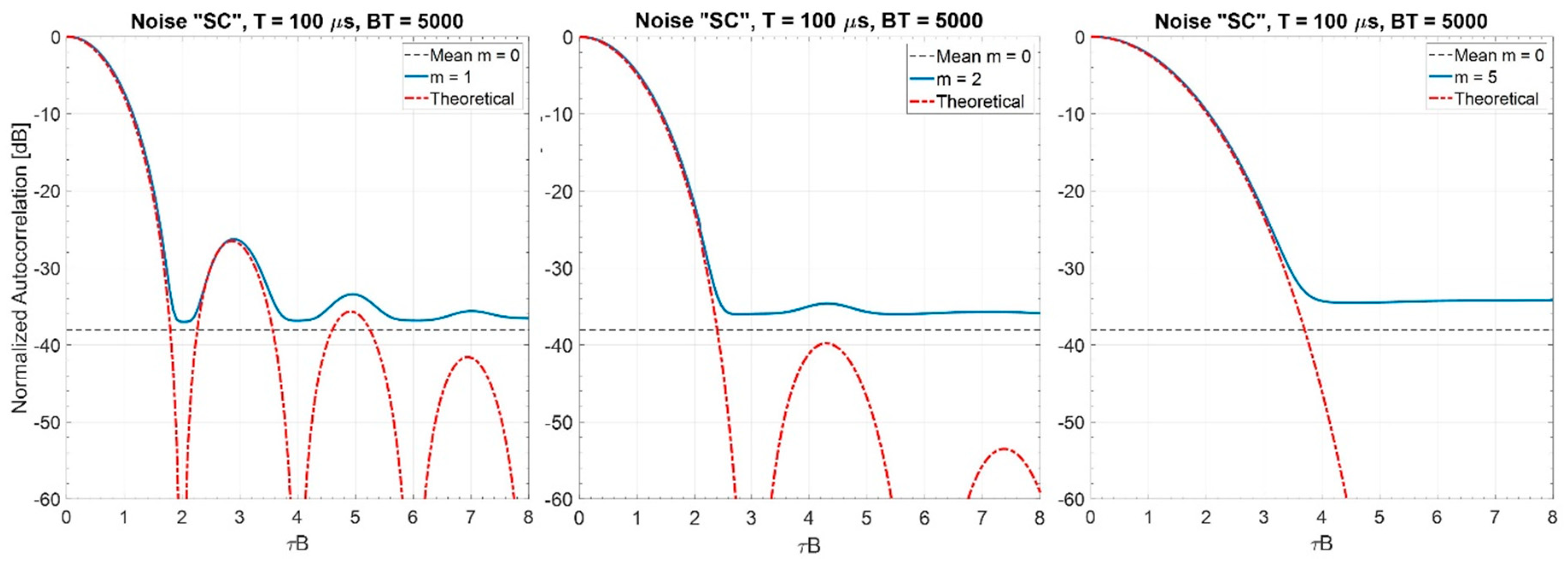
- the mean value of the is (regardless of ), a value very close to corresponding to .
2.2.3. The Range Transition Zone
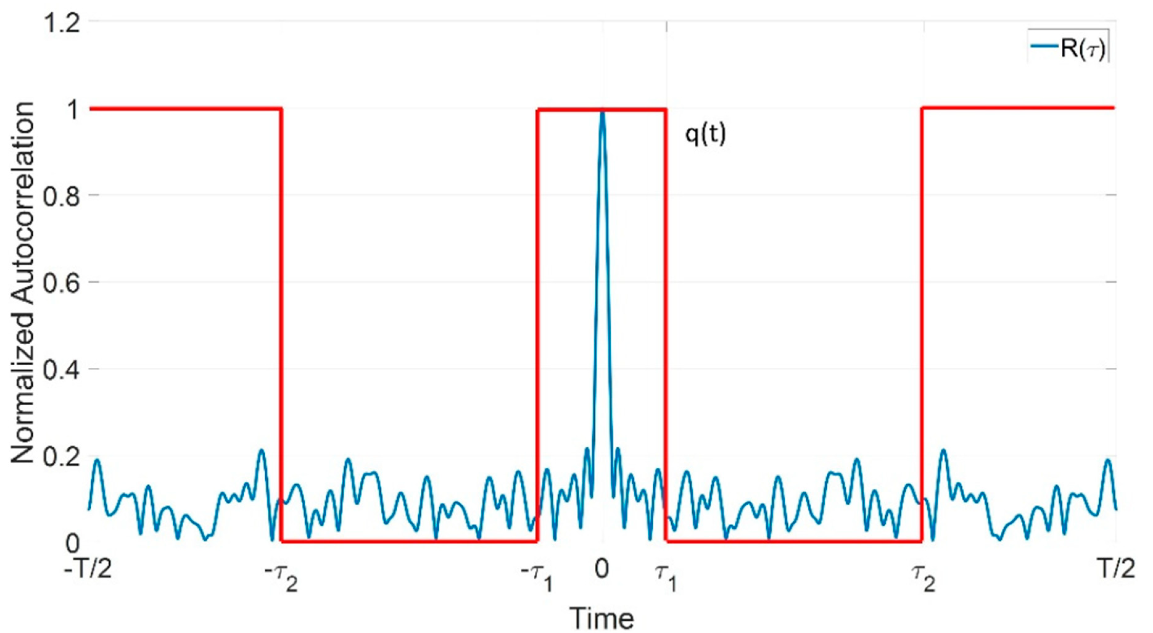
3. Range Sidelobes Suppression for the Autocorrelation Function of Noise Waveforms
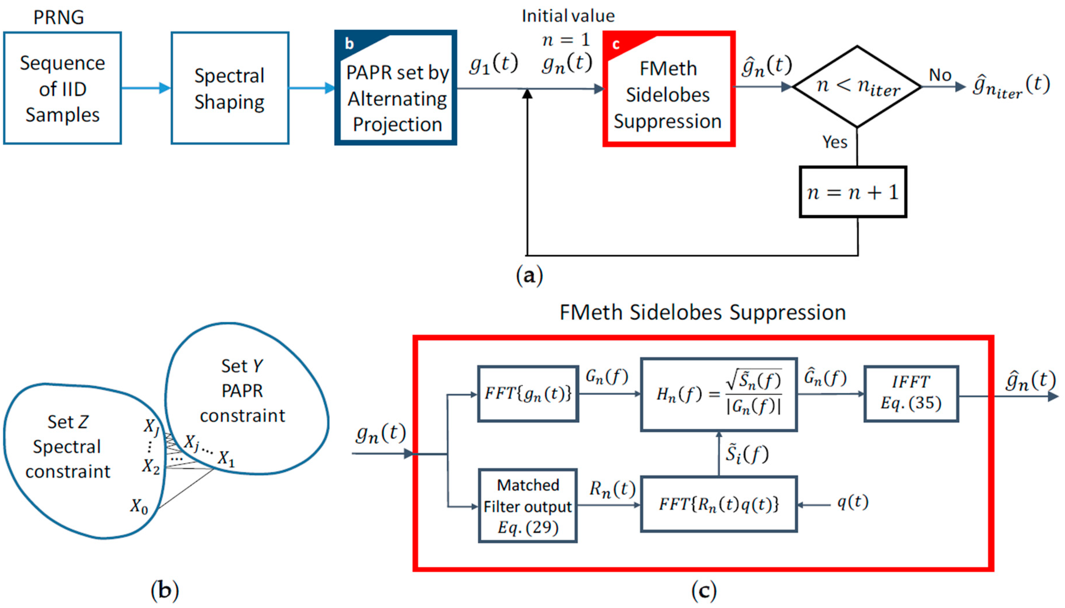
3.1. The FMeth (Filtering Method) Algorithm: General Description
3.1.1. PRNG and Spectral Shaping
3.1.2. PAPR Setting by Alternating Projection
3.1.3. FMeth Sidelobes Suppression
- The sample autocorrelation of the PAPR-regulated sequence is computed.
- Zeroing the points of between and by multiplication with , Equation (31), the desired autocorrelation is determined.
- The spectrum and the Fourier transform of are estimated by FFT, and, from Equation (34), the frequency response is evaluated.
- The random signal , whose autocorrelation function shows attenuated sidelobes inside the time interval , is generated by the following procedure:
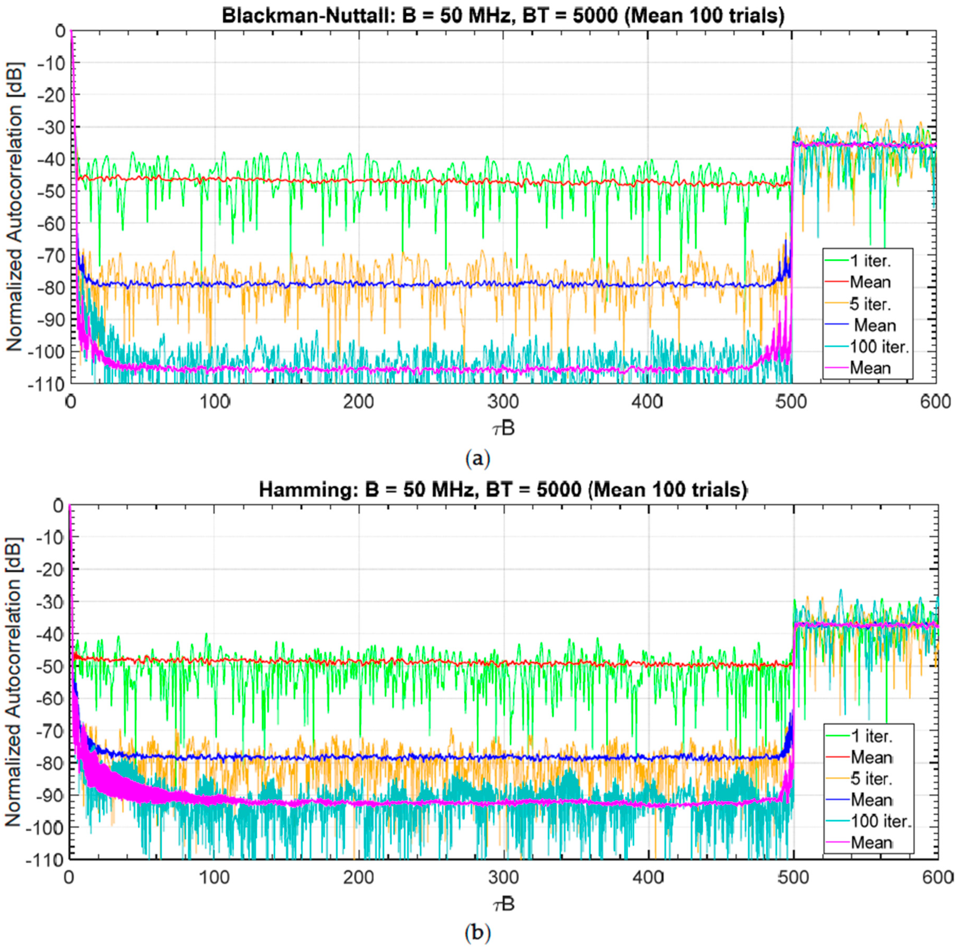
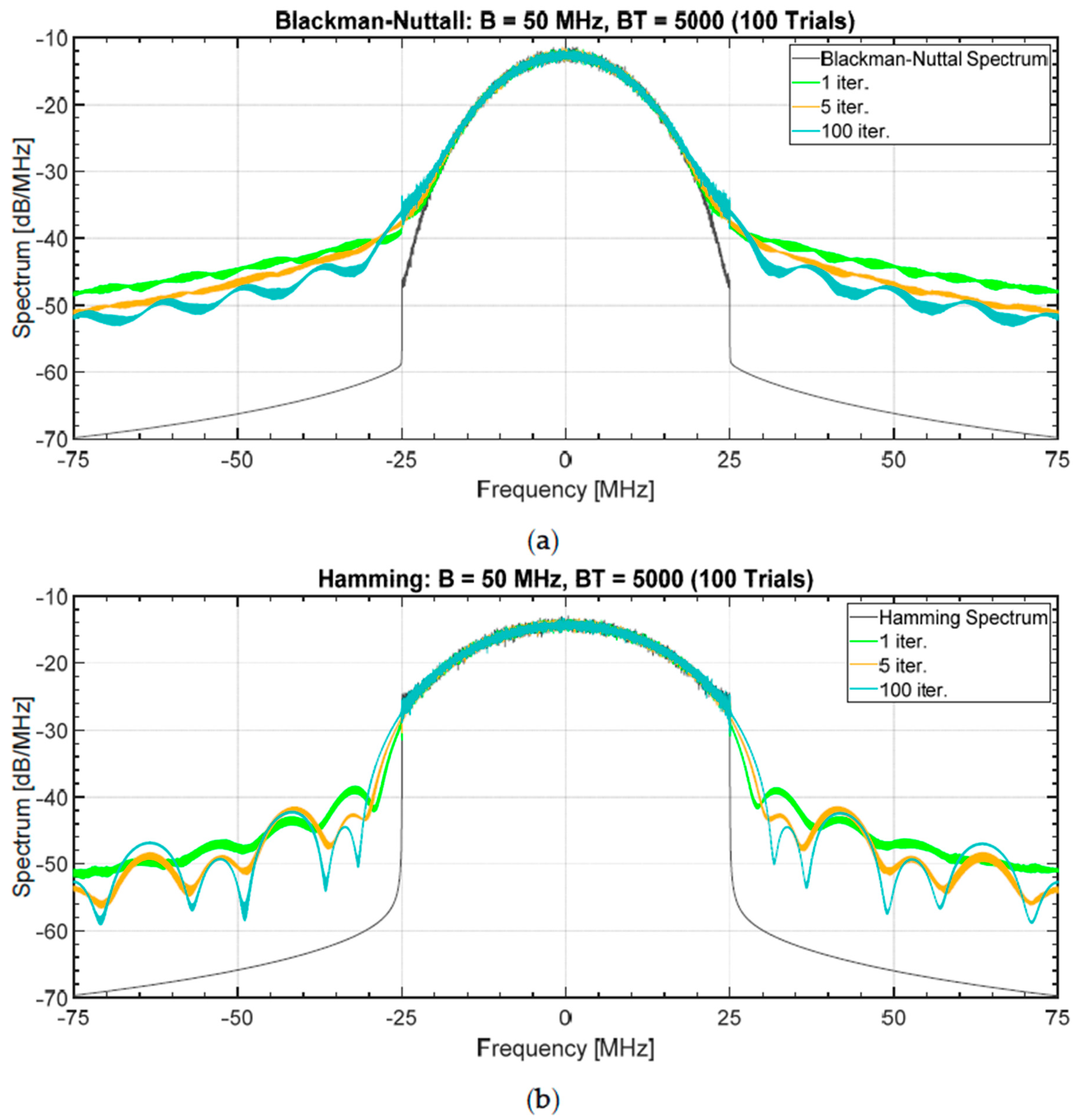
3.2. Results for Zero Doppler–Sidelobes Level in the ACF
3.2.1. Sensitivity of the Sidelobe Attenuation to the Number of Iterations
3.2.2. Sensitivity of the Sidelobe Attenuation to the PAPR and to the Width of the Suppression Zone
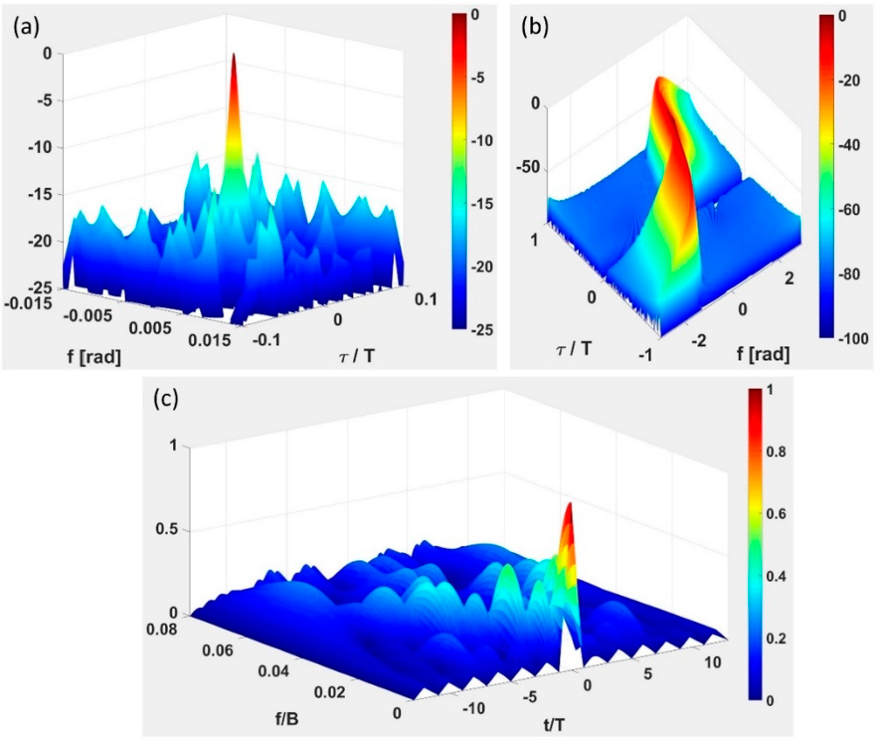
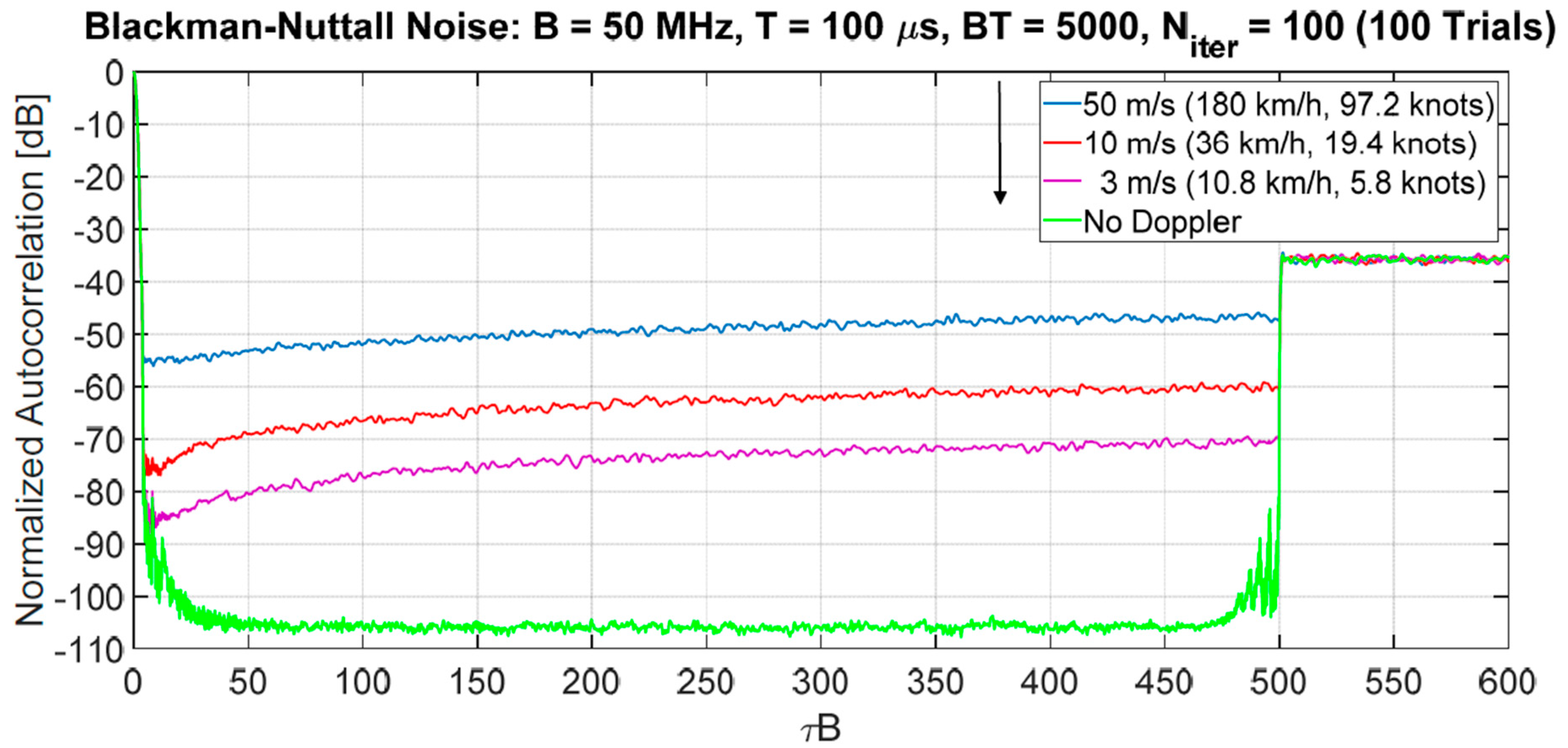
3.3. Doppler Sensitivity and Sidelobes Suppression for the Ambiguity Function
4. Comments, Conclusions, and Short Reference to Future Experimental Work
Author Contributions
Funding
Conflicts of Interest
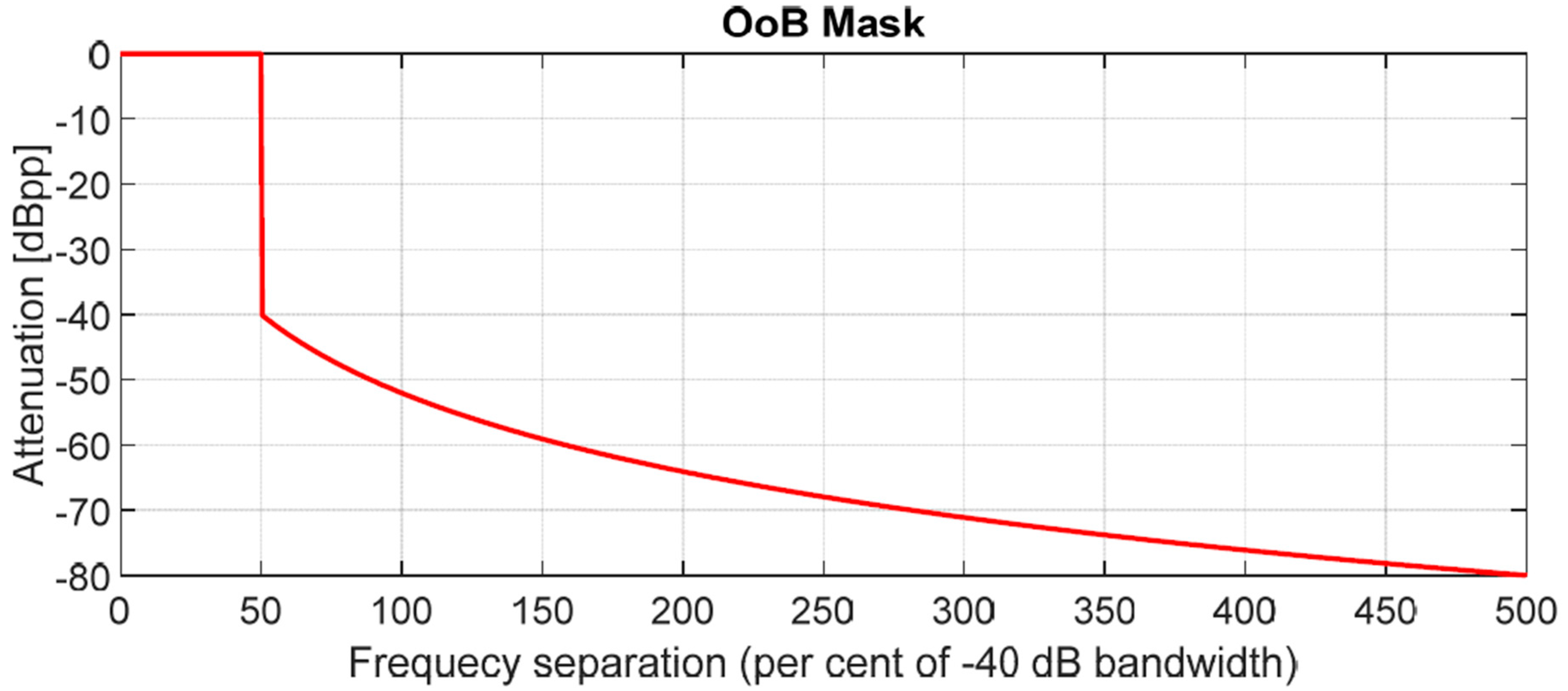
Appendix A. Band Occupancy in NRT Applications

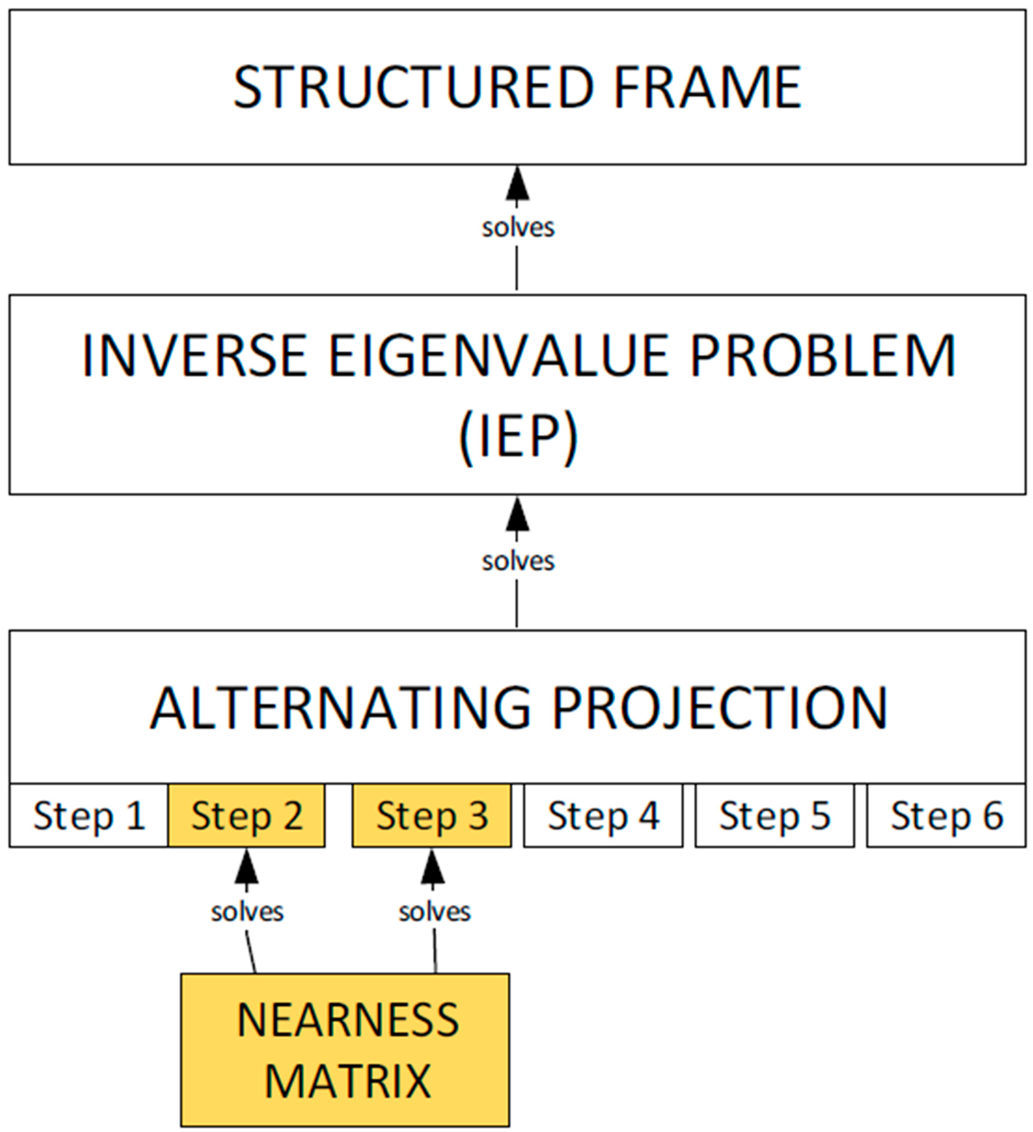
Appendix B. The “Alternating Projection” Algorithm
- An (arbitrary) initial matrix
- The number of the iteration,
- A matrix in and a matrix in
- (1)
- Initialize
- (2)
- Find a matrix in such thatbeing operator the Frobenius norm.
- (3)
- Find a matrix in such that
- (4)
- Increment by one.
- (5)
- Repeat steps 2–4 until
- (6)
- Let and

References
- Levanon, N.; Mozeson, E. Radar Signals; John Wiley & Sons, Inc.: Hoboken, NJ, USA, 2004. [Google Scholar]
- Cook, C.E.; Bernfeld, M. Radar Signals: An Introduction to Theory and Applications; Artech House, Inc.: Norwood, MA, USA, 1993. [Google Scholar]
- Horton, B.M. Noise-modulated distance measuring system. IRE Proc. 1959, 49, 821–828. [Google Scholar] [CrossRef]
- De Martino, A. Introduction to Modern EW Systems, 2nd ed.; Artech House, Inc.: Norwood, MA, USA, 2018. [Google Scholar]
- Galati, G.; Pavan, G.; De Palo, F. Compatibility problems related with pulse-compression, solid-state marine radars. IET Radar Sonar Navig. 2016, 10, 791–797. [Google Scholar] [CrossRef]
- Achatz, R.J. Method for Evaluating Solid State Marine Radar Interference in Magnetron Marine Radars. In Proceedings of the IEEE Radar Conference 2019 (RadarConf), Boston, MA, USA, 22–26 April 2019. [Google Scholar] [CrossRef]
- Galati, G.; Pavan, G.; De Palo, F.; Stove, A. Potential applications of noise radar technology and related waveform diversity. In Proceedings of the 17th International Radar Symposium (IRS 2016), Krakow, Poland, 10–12 May 2016. [Google Scholar] [CrossRef]
- Henel, S. Automotive Radar Interference Test. In Proceedings of the 18th International Radar Symposium (IRS 2017), Prague, Czech Republic, 20–30 June 2017. Edited by DGON. [Google Scholar] [CrossRef]
- Recommendation ITU-R SM.1541-6. Unwanted Emissions in the Out-Of-Band Domain, SM Series: Spectrum Management, Annex 8; ITU: Geneva, Switzerland, 2015; pp. 49–56. [Google Scholar]
- Baker, C.J.; Piper, S.O. Continuous Wave Radar. In Principles of Modern Radar, vol. 3 Radar Applications; IET Digital Library: London, UK, 2014; Chapter 2. [Google Scholar] [CrossRef]
- Melvin, W.L.; Scheer, J. Principles of Modern Radar: Radar Applications; Scitech Publishing: Edison, NJ, USA, 2013. [Google Scholar]
- Malanowski, M.; Kulpa, K. Detection of Moving Targets with Continuous Wave Noise Radar: Theory and Measurements. IEEE Trans. Geosci. Remote Sens. 2012, 50, 3502–3509. [Google Scholar] [CrossRef]
- Gentle, J.E. Random Number Generators and Monte Carlo Methods, 2nd ed.; Springer: Berlin, Germany, 2003. [Google Scholar]
- Mersenne Twister Home Page: A Very Fast Random Number Generator of Period 219937-1. Available online: http://www.math.sci.hiroshima-u.ac.jp/~m-mat/MT/emt.html (accessed on 30 July 2020).
- He, H.; Li, J.; Stoica, P. Waveform Design for Active Sensing Systems—A Computational Approach; Cambridge University Press: Cambridge, MA, USA, 2012. [Google Scholar]
- De Palo, F.; Galati, G. Range sidelobes attenuation of pseudorandom waveforms for civil radars. In Proceedings of the European Radar Conference 2017, Nuremberg, Germany, 11–13 October 2017. [Google Scholar] [CrossRef]
- Fisher, R.A. Frequency Distribution of the Values of the Correlation Coefficient in Samples from an Indefinitely Large Population. Biometrika 1915, 10, 507–521. [Google Scholar] [CrossRef]
- Galati, G.; Pavan, G.; Wasserzier, C. Continuous—Emission Noise Radar: Design Criteria and Waveforms. In Proceedings of the IEEE 7th International Workshop on Metrology for AeroSpace (MetroAeroSpace), Pisa, Italy, 20–22 June 2020; pp. 154–159. [Google Scholar] [CrossRef]
- Nuttall, A.H. Some Windows with Very Good Sidelobe Behaviour. IEEE Trans. Acoust. Speech Signal Process. 1981, 29, 84–91. [Google Scholar] [CrossRef]
- Kulpa, J.S. Mismatched Filter for Range Sidelobes Suppression of Pseudo-Noise Signals. In Proceedings of the Signal Processing Symposium (SPSympo) 2015, Debe, Poland, 10–12 June 2015; 10–12 June 2015. [Google Scholar] [CrossRef]
- Kulpa, J.S.; Maslikowski, L.; Malanowski, M. Filter-Based Design of Noise Radar Waveform with Reduced Sidelobes. IEEE Trans. Aerosp. Electron. Syst. 2017, 53, 816–825. [Google Scholar] [CrossRef]
- Yang, Q.; Zhang, Y.; Gu, X. Design of ultralow sidelobe chaotic radar signal by modulating group delay method. IEEE Trans. Aerosp. Electron. Syst. 2015, 51, 3023–3035. [Google Scholar] [CrossRef]
- Tohidi, E.; Nazari Majd, M.; Bahadori, M.; Haghshenas Jariani, M.; Nayebi, M.M. Periodicity in Contrast with Sidelobe Suppression in Random Signal Radars. In Proceedings of the IEEE CIE International Conference on Radar, Chengdu, China, 24–27 October 2011. [Google Scholar] [CrossRef]
- Tropp, J.A.; Dhillon, I.S.; Heath, R.W.; Strohmer, T. Designing Structured Tight Frames Via an Alternating Projection Method. IEEE Trans. Inf. Theory 2005, 51, 188–209. [Google Scholar] [CrossRef]
- Christensen, O. An Introduction to Frames and Riesz Bases, 2nd ed.; Birkhäuser: Boston, MA, USA, 2003. [Google Scholar]
- Wasserzier, C.; Galati, G. On the efficient computation of range and Doppler data in noise radar. Int. J. Microw. Wirel. Technol. 2019, 11, 584–592. [Google Scholar] [CrossRef]
- Wasserzier, C. Noise Radar on Moving Platforms; Ph.D. Thesis, Tor Vergata University, XXXII Cycle; TEXMAT: Rome, Italy, 2020; ISBN 978-88-949-8235-0. [Google Scholar]
- O’Donnell, R.M.; Muehe, C.E. Automated Tracking for Aircraft Surveillance Radar Systems. IEEE Trans. Aerosp. Electron. Syst. 1979, AES-15, 508–517. [Google Scholar]
- D’Addio, E.; Galati, G. Adaptivity and design criteria of a latest-generation MTD processor. IEE Proc. Part F Commun. Radar Signal Process. 1985, 132, 58–65. [Google Scholar] [CrossRef]
- Higham, N.J. Matrix nearness problems and applications. In Applications of Matrix Theory; Gover, M.J.C., Barnett, S., Eds.; Oxford University Press: Oxford, UK, 1989; pp. 1–27. [Google Scholar]


| PAPR | Loss (dB) |
|---|---|
| 1.0 | 0.0 |
| 1.25 | 0.97 |
| 1.5 | 1.76 |
| 1.75 | 2.43 |
| 2.0 | 3.01 |
| 3.0 | 4.77 |
| 5.0 | 6.99 |
| 7.0 | 8.45 |
| 10.0 | 10.0 |
| “NV” Waveforms | |||||
|---|---|---|---|---|---|
| m | B−3/B | B−6/B | B−10/B | B−20/B | B−40/B |
| 1 | 0.67 | 1.06 | 1.27 | 1.34 | 1.41 |
| 2 | 0.73 | 1.02 | 1.28 | 1.42 | 1.72 |
| 3 | 0.72 | 1.00 | 1.26 | 1.42 | 1.93 |
| 4 | 0.70 | 0.98 | 1.25 | 1.68 | 2.06 |
| 5 | 0.71 | 0.99 | 1.24 | 1.41 | 2.15 |
| 10 | 0.69 | 0.98 | 1.25 | 1.41 | 2.32 |
| “SC” Waveforms | ||||
|---|---|---|---|---|
| m | B−3/B | B−6/B | B−10/B | B−20/B |
| 1 | 0.50 | 0.75 | 0.90 | 0.95 |
| 2 | 0.42 | 0.59 | 0.74 | 0.82 |
| 3 | 0.36 | 0.50 | 0.63 | 0.71 |
| 5 | 0.29 | 0.40 | 0.51 | 0.58 |
| 10 | 0.21 | 0.29 | 0.38 | 0.43 |
| Suppression Zone [%] | PAPR 9.0 | PAPR 5.0 | PAPR 2.0 | PAPR 1.5 | PAPR 1.0 |
|---|---|---|---|---|---|
| 20 | −103.9 | −100.8 | −89.3 | −75.9 | −57.9 |
| 40 | −104.3 | −101.1 | −79.6 | −66.3 | −54.5 |
| 60 | −102.5 | −95.2 | −71.1 | −60.7 | −52.3 |
| 80 | −99.7 | −88.6 | −63.0 | −56.9 | −51.5 |
| 95 | −89.1 | −78.3 | −58.8 | −55.1 | −50.6 |
| 100 | −83.1 | −69.5 | −56.5 | −53.8 | −49.9 |
| Suppression Zone [%] | PAPR 9.0 | PAPR 5.0 | PAPR 2.0 | PAPR 1.5 | PAPR 1.0 |
|---|---|---|---|---|---|
| 20 | −92.3 | −93.6 | −89.9 | −76.8 | −59.3 |
| 40 | −90.7 | −93.3 | −80.3 | −67.5 | −56.0 |
| 60 | −88.4 | −89.1 | −71.7 | −61.9 | −54.0 |
| 80 | −84.0 | −82.9 | −64.3 | −58.3 | −52.9 |
| 95 | −79.2 | −74.9 | −60.2 | −56.4 | −52.2 |
| 100 | −73.1 | −68.3 | −58.2 | −55.0 | −51.4 |
© 2020 by the authors. Licensee MDPI, Basel, Switzerland. This article is an open access article distributed under the terms and conditions of the Creative Commons Attribution (CC BY) license (http://creativecommons.org/licenses/by/4.0/).
Share and Cite
Palo, F.D.; Galati, G.; Pavan, G.; Wasserzier, C.; Savci, K. Introduction to Noise Radar and Its Waveforms. Sensors 2020, 20, 5187. https://doi.org/10.3390/s20185187
Palo FD, Galati G, Pavan G, Wasserzier C, Savci K. Introduction to Noise Radar and Its Waveforms. Sensors. 2020; 20(18):5187. https://doi.org/10.3390/s20185187
Chicago/Turabian StylePalo, Francesco De, Gaspare Galati, Gabriele Pavan, Christoph Wasserzier, and Kubilay Savci. 2020. "Introduction to Noise Radar and Its Waveforms" Sensors 20, no. 18: 5187. https://doi.org/10.3390/s20185187
APA StylePalo, F. D., Galati, G., Pavan, G., Wasserzier, C., & Savci, K. (2020). Introduction to Noise Radar and Its Waveforms. Sensors, 20(18), 5187. https://doi.org/10.3390/s20185187