Prognosis of Bearing and Gear Wears Using Convolutional Neural Network with Hybrid Loss Function


Abstract
1. Introduction
2. One-Dimensional Convolutional Neural Network (1-D CNN) with Clustering Loss for Prognosis
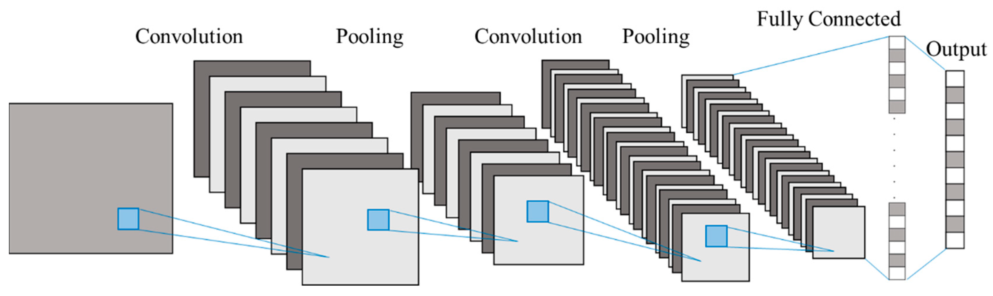
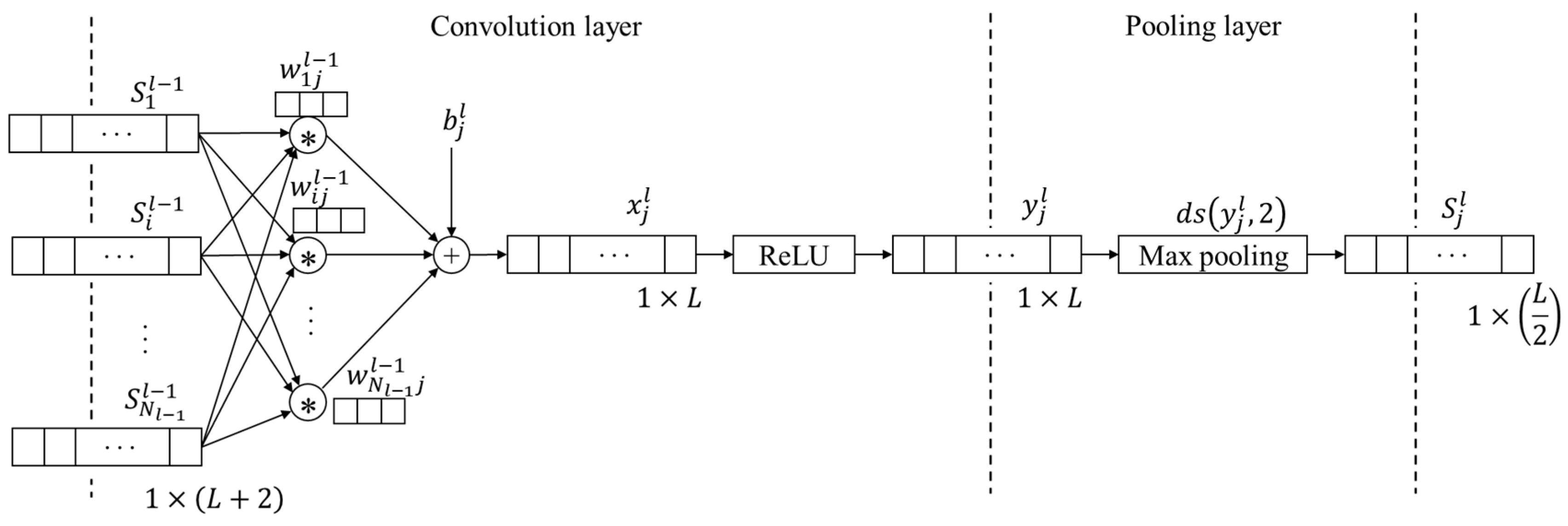
2.1. One-Dimensional Convolutional Neural Network
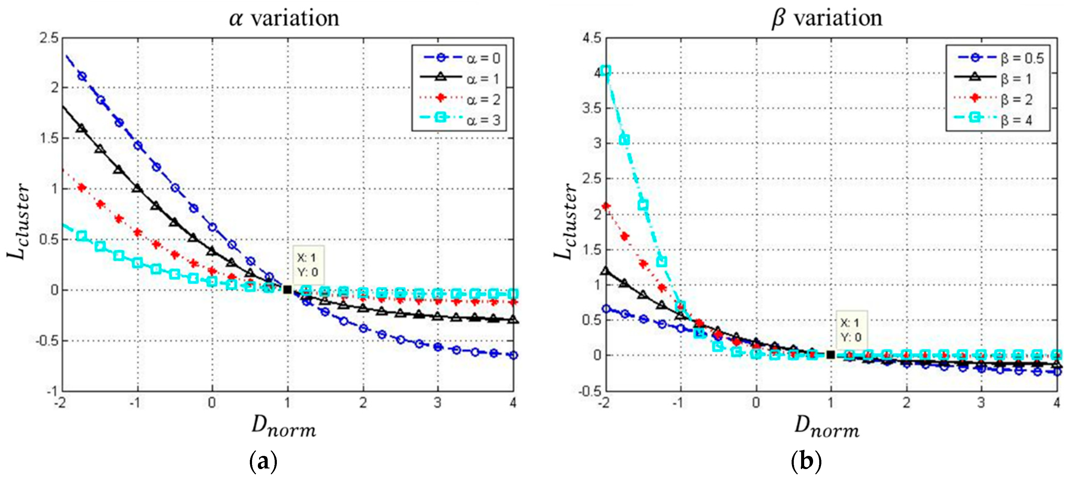
2.2. Clustering Loss
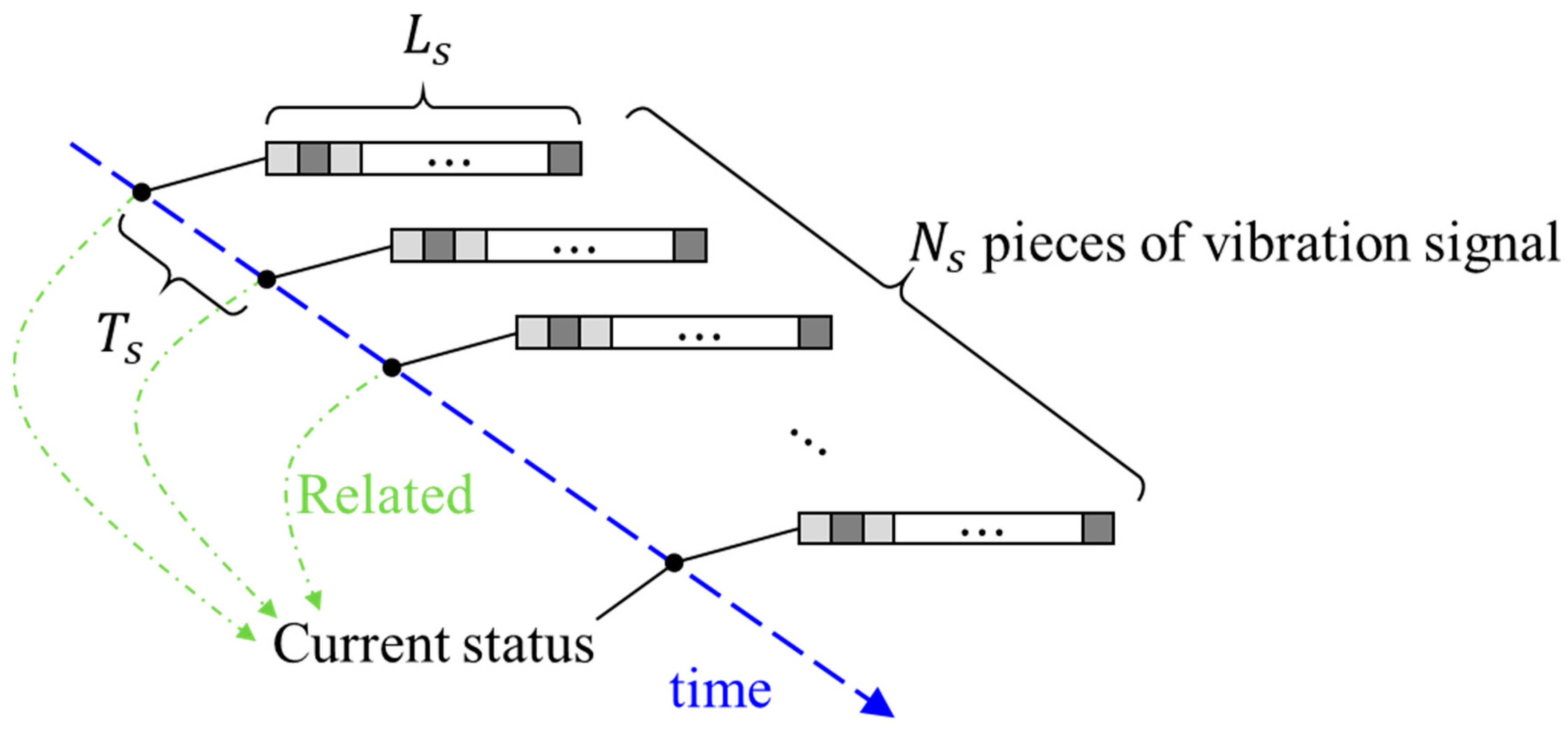
2.3. Time Series Input
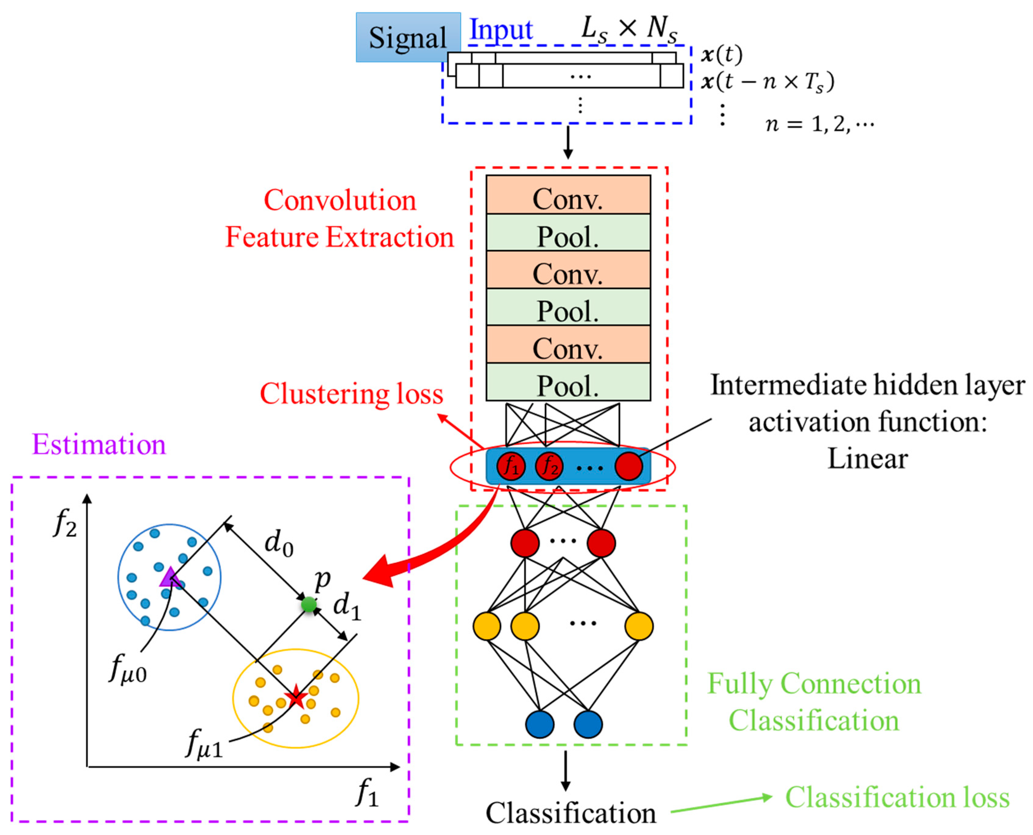
2.4. The Proposed Approach for Prognosis Approach
3. Analysis and Validation: IEEE Prognostics and Health Management (PHM) Open Dataset
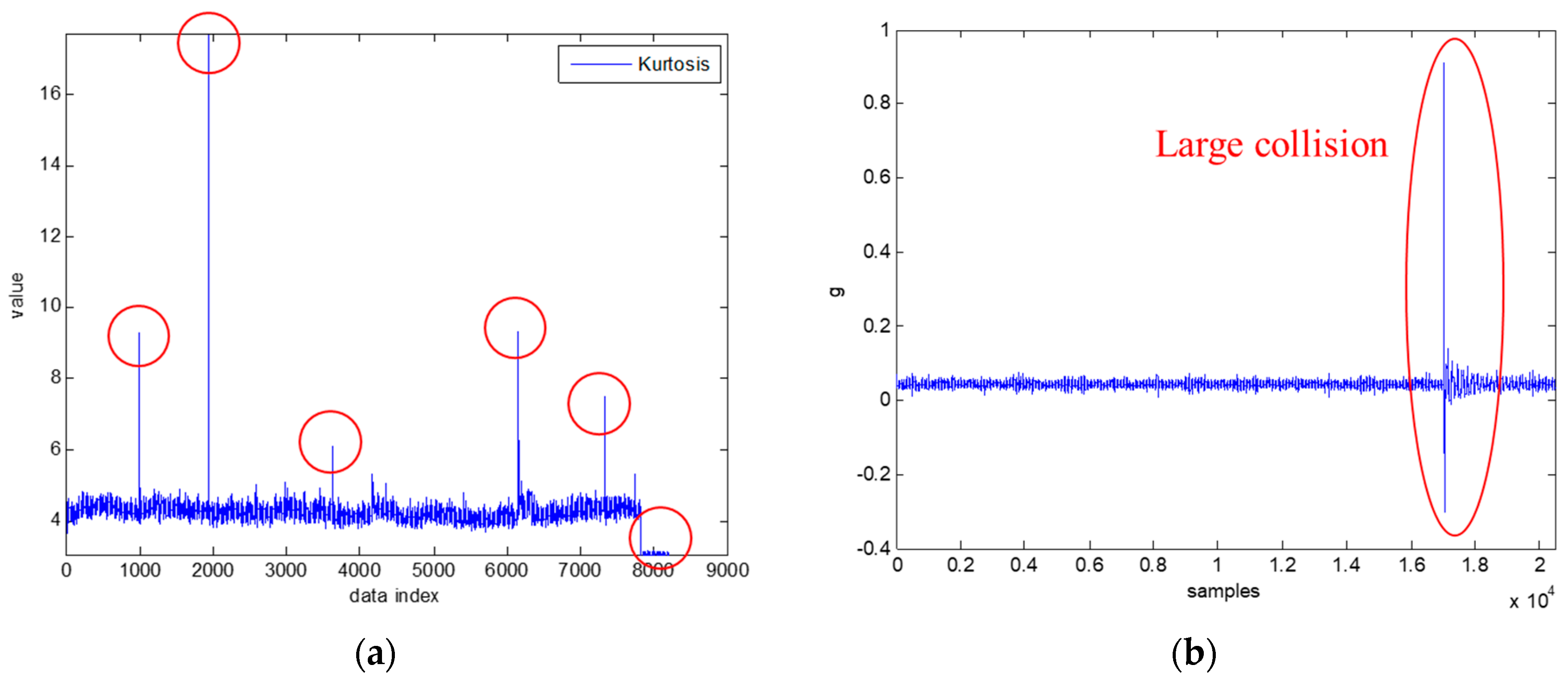
3.1. Data Acquirement and Processing
3.2. 1-D CNN with Clustering Loss Model Analysis
4. Experimental Results: Gear Wear
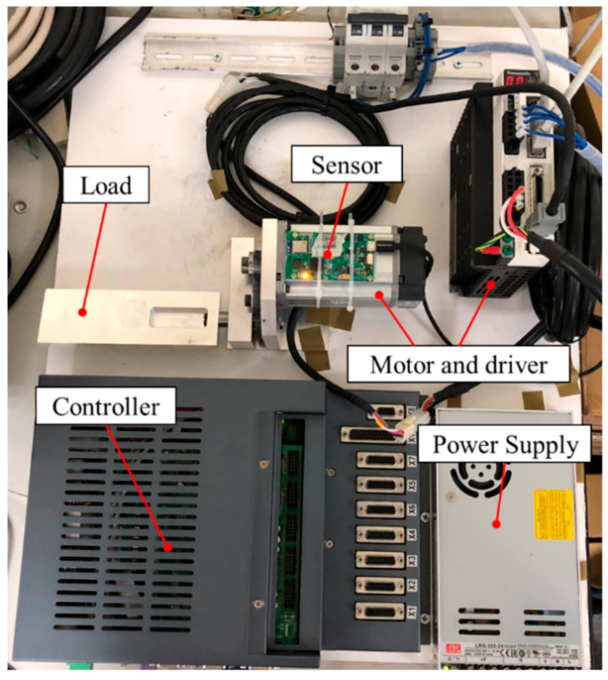
4.1. Experimental Platform Setup
4.2. Gear Wear Data Acquisition
- G90G54X0.F300.
- #31 = 30,000
- N1
- IF[#31 <=0]GOTO2
- G91 X +5. F300.
- G04 X0.3
- G91 X -5. F300.
- G04 X0.3
- #31 = #31-1
- GOTO1
- N2
- M30
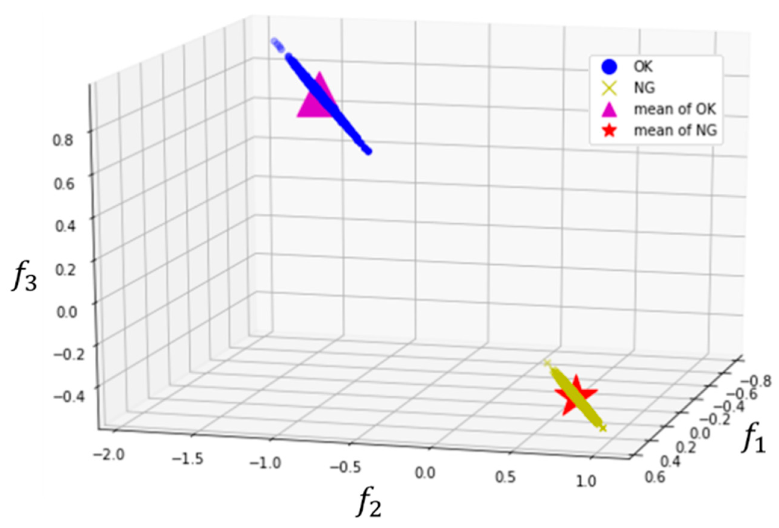
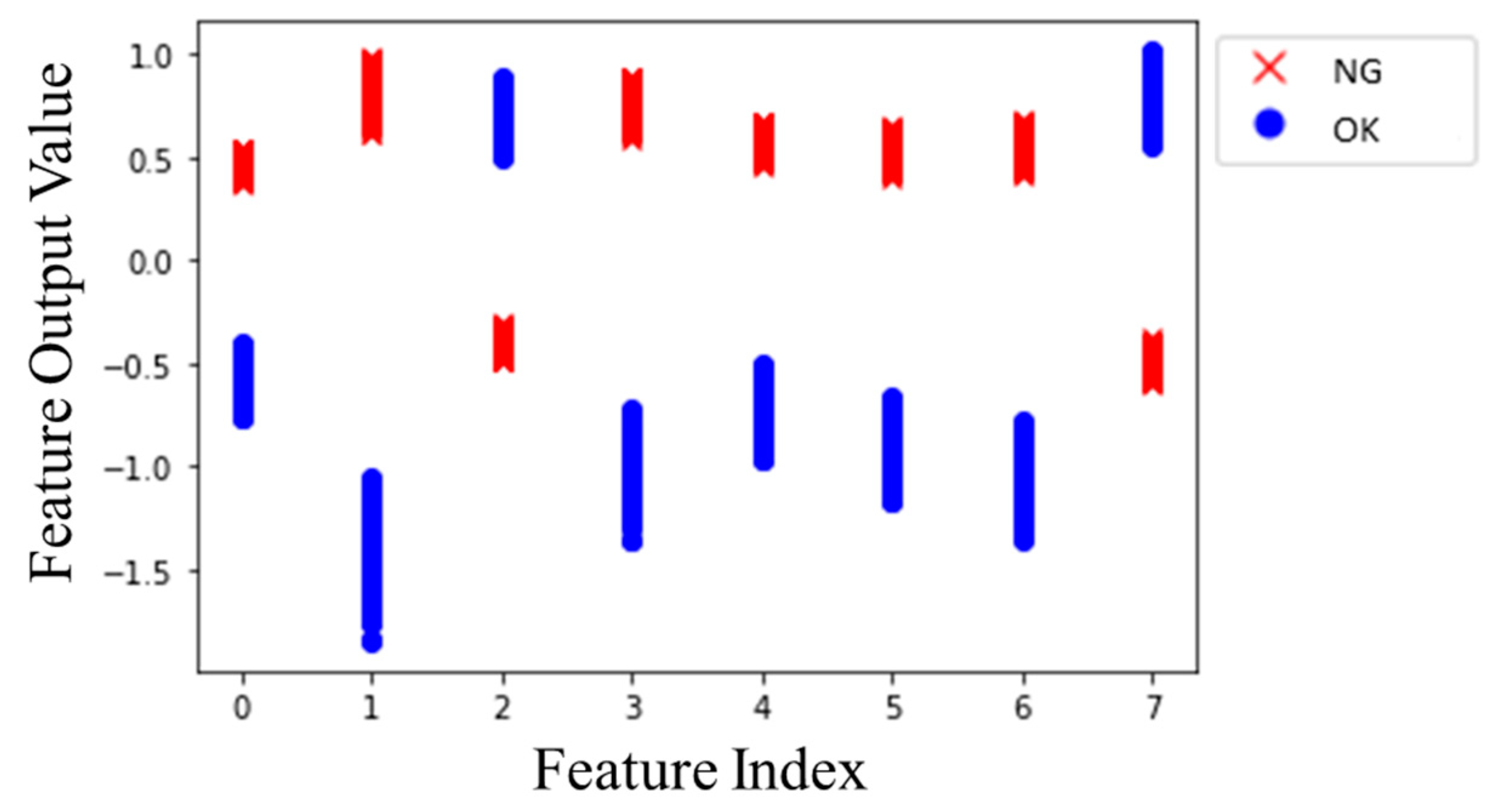
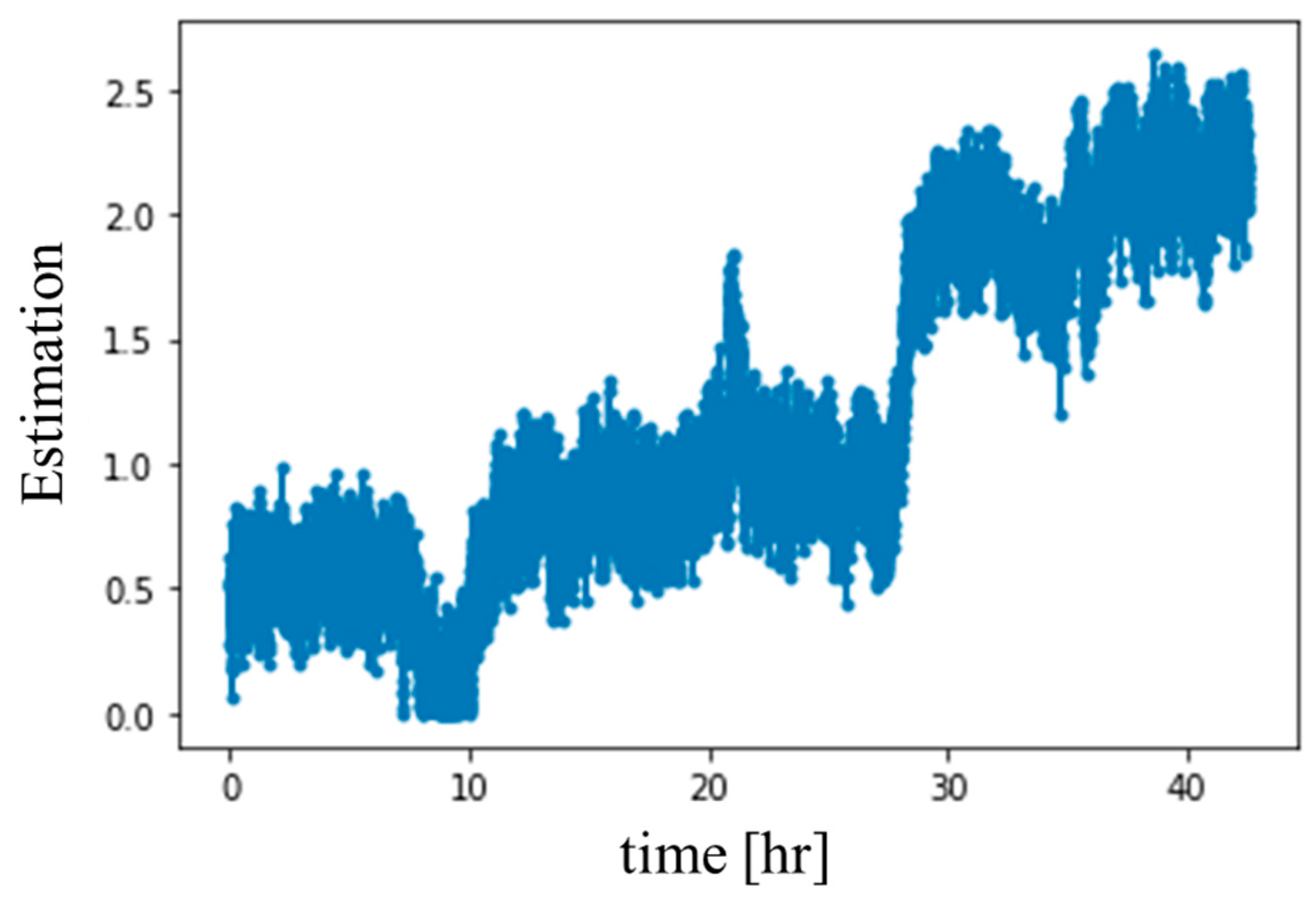
4.3. Experimental Results
5. Conclusions
Author Contributions
Funding
Acknowledgments
Conflicts of Interest
References
- Lee, J.; Wu, F.; Zhao, W.; Ghaffari, M.; Liao, L.; Siegel, D. Prognostics and Health Management Design for Rotary Machinery Systems—Reviews, Methodology and Applications. Mech. Syst. Signal Process. 2014, 42, 314–334. [Google Scholar] [CrossRef]
- Rangel-Magdaleno, J.; Peregrina-Barreto, H.; Ramirez-Cortes, J.; Cruz-Vega, I. Hilbert Spectrum Analysis of Induction Motors for the Detection of Incipient Broken Rotor Bars. Measurement 2017, 109, 247–255. [Google Scholar] [CrossRef]
- Jin, X.; Sun, Y.; Que, Z.; Wang, Y.; Chow, T.W. Anomaly Detection and Fault Prognosis for Bearings. IEEE Trans. Instrum. Meas. 2016, 65, 2046–2054. [Google Scholar] [CrossRef]
- Zhang, R.; Gu, F.; Mansaf, H.; Wang, T.; Ball, A.D. Gear Wear Monitoring by Modulation Signal Bispectrum Based on Motor Current Signal Analysis. Mech. Syst. Signal Process. 2017, 94, 202–213. [Google Scholar] [CrossRef]
- Lei, Y.; Li, N.; Guo, L.; Li, N.; Yan, T.; Lin, J. Machinery Health Prognostics: A Systematic Review from Data Acquisition to RUL Prediction. Mech. Syst. Signal Process. 2018, 104, 799–834. [Google Scholar] [CrossRef]
- Guo, L.; Li, N.; Jia, F.; Lei, Y.; Lin, J. A Recurrent Neural Network Based Health Indicator for Remaining Useful Life Prediction of Bearings. Neurocomputing 2017, 240, 98–109. [Google Scholar] [CrossRef]
- Zhao, R.; Yan, R.; Chen, Z.; Mao, K.; Wang, P.; Gao, R.X. Deep Learning and Its Applications to Machine Health Monitoring. Mech. Syst. Signal Process. 2019, 115, 213–237. [Google Scholar] [CrossRef]
- Yao, Y.; Wang, H.; Li, S.; Liu, Z.; Gui, G.; Dan, Y.; Hu, J. End-to-end Convolutional Neural Network Model for Gear Fault Diagnosis Based on Sound Signals. Appl. Sci. 2018, 8, 1584. [Google Scholar] [CrossRef]
- Sohaib, M.; Kim, C.-H.; Kim, J.-M. A Hybrid Feature Model and Deep-Learning-based Bearing Fault Diagnosis. Sensors 2017, 17, 2876. [Google Scholar] [CrossRef] [PubMed]
- Hoang, D.T.; Kang, H.J. Rolling Element Bearing Fault Diagnosis Using Convolutional Neural Network and Vibration Image. Cogn. Syst. Res. 2019, 53, 42–50. [Google Scholar] [CrossRef]
- Min, E.; Guo, X.; Liu, Q.; Zhang, G.; Cui, J.; Long, J. A Survey of Clustering with Deep Learning: From the Perspective of Network Architecture. IEEE Access 2018, 6, 39501–39514. [Google Scholar] [CrossRef]
- Aljalbout, E.; Golkov, V.; Siddiqui, Y.; Strobel, M.; Cremers, D. Clustering with Deep Learning: Taxonomy and New Methods. arXiv 2018, arXiv:1801.07648. [Google Scholar]
- Hong, S.; Zhou, Z.; Zio, E.; Hong, K. Condition Assessment for the Performance Degradation of Bearing Based on a Combinatorial Feature Extraction Method. Digit. Signal Process. 2014, 27, 159–166. [Google Scholar] [CrossRef]
- Yang, C.; Wu, T. Diagnostics of Gear Deterioration Using EEMD Approach and PCA Process. Measurement 2015, 61, 75–87. [Google Scholar] [CrossRef]
- Zhao, H.; Deng, W.; Yang, X.; Li, X. Research on a Vibration Signal Analysis Method for Motor Bearing. Optik 2016, 127, 10014–10023. [Google Scholar] [CrossRef]
- Chen, X.; Feng, F.; Zhang, B. Weak Fault Feature Extraction of Rolling Bearings Based on an Improved Kurtogram. Sensors 2016, 16, 1482. [Google Scholar] [CrossRef] [PubMed]
- Sinha, A. Vibration of Mechanical Systems; Cambridge University Press: New York, NY, USA, 2010; pp. 271–322. [Google Scholar]
- Ren, S.; He, K.; Girshick, R.; Sun, J. Faster R-CNN: Towards Real-Time Object Detection with Region Proposal Networks. In Advances in Neural Information Processing Systems; Neural Information Processing Systems Foundation, Inc.: Montreal, QC, Canada, 2015; pp. 91–99. [Google Scholar]
- Krizhevsky, A.; Sutskever, I.; Hinton, G.E. Imagenet classification with deep convolutional neural networks. In Advances in Neural Information Processing Systems; Neural Information Processing Systems Foundation, Inc.: Montreal, QC, Canada, 2012; pp. 1097–1105. [Google Scholar]
- Gu, J.; Wang, Z.; Kuen, J.; Ma, L.; Shahroudy, A.; Shuai, B.; Liu, T.; Wang, X.; Wang, G.; Cai, J. Recent Advances in Convolutional Neural Networks. Pattern Recognit. 2018, 77, 354–377. [Google Scholar] [CrossRef]
- Ince, T.; Kiranyaz, S.; Eren, L.; Askar, M.; Gabbouj, M. Real-time Motor Fault Detection by 1-D Convolutional Neural Networks. IEEE Trans. Ind. Electron. 2016, 63, 7067–7075. [Google Scholar] [CrossRef]
- Lo, C.C.; Chen, B.S.; Lee, C.H. Fault Detection and Remaining Useful Life Estimation of Bearing Using Deep Learning Approach. In Proceedings of the International Conference on Advanced Robotics and Intelligent Systems, Taipei, Taiwan, 20–23 August 2019. [Google Scholar]
- Feng, K.; Borghesani, P.; Smith, W.A.; Randall, R.B.; Chin, Z.Y.; Ren, J.; Peng, Z. Vibration-based updating of wear prediction for spur gears. Wear 2019, 426, 1410–1415. [Google Scholar] [CrossRef]
- Nectoux, P.; Gouriveau, R.; Medjaher, K.; Ramasso, E.; Chebel-Morello, B.; Zerhouni, N.; Varnier, C. PRONOSTIA: An Experimental Platform for Nearings Accelerated Degradation Tests. In Proceedings of the 2012 IEEE Conference on Prognostics and Health Management, PHM’12, Denver, CO, USA, 18–21 June 2012; 2012; pp. 1–8. [Google Scholar]
- Gimpert, D. A New Standard in Gear Inspection. Gear Solutions, October 2005; 35–38. [Google Scholar]


| Algorithm and Parameters | Values |
|---|---|
| Learning algorithm | Adam |
| Initial learning rate | 0.0001 |
| Decay | 0 |
| Learning epochs | 1000 |
| Batch learning size | 64 |
| α | 2 |
| β | 1 |
| Adam | Rmsprop | Adagrad | Momentum | Gradient Descent | |
|---|---|---|---|---|---|
| Initial learning rate | 0.0001 | ||||
| Epoch number | 1000 | ||||
| Clustering loss | 0.007 | 0.012 | 0.099 | 0.061 | 0.130 |
| Classify loss | 0.314 | 0.314 | 0.694 | 0.693 | 0.694 |
| Train data accuracy | 100.00% | 99.91% | 10.13% | 50.00% | 50.00% |
| Val. data accuracy | 99.61% | 99.65% | 12.11% | 50.00% | 50.00% |
| Test data accuracy | 91.29% | 50.00% | 50.00% | 50.00% | 50.00% |
| Model | (2, 2) | (3, 2) | (4, 2) | (5, 2) | (6, 2) | (7, 2) | (8, 2) | |
| Accuracy | Training | 99.96% | 99.96% | 99.92% | 100.00% | 99.92% | 100.00% | 99.92% |
| Validation | 99.48% | 99.65% | 99.83% | 99.13% | 99.65% | 99.83% | 99.83% | |
| Testing | 92.00% | 89.70% | 91.23% | 91.02% | 91.39% | 82.30% | 86.43% | |
| Model | (2, 5) | (3, 5) | (4, 5) | (5, 5) | (6, 5) | (7, 5) | (2, 10) | |
| Accuracy | Training | 100.00% | 99.92% | 99.96% | 99.96% | 100.00% | 99.96% | 100.00% |
| Validation | 99.83% | 100.00% | 100.00% | 99.80% | 99.80% | 99.48% | 99.48% | |
| Testing | 91.93% | 91.29% | 91.29% | 87.50% | 91.36% | 91.42% | 88.78% | |
| Model | (3,10) | (4, 10) | (5, 10) | (6, 10) | (2, 20) | (3, 20) | (4, 20) | |
| Accuracy | Training | 99.92% | 99.96% | 100.00% | 99.91% | 99.96% | 99.96% | 99.91% |
| Validation | 99.80% | 99.61% | 99.61% | 100.00% | 99.65% | 100.00% | 100.00% | |
| Testing | 90.31% | 91.10% | 91.29% | 87.40% | 90.94% | 92.09% | 91.07% | |
| Model | (5, 20) | (2, 40) | (3, 40) | (4, 40) | (2, 60) | (3, 60) | (2, 80) | |
| Accuracy | Training | 99.95% | 99.96% | 99.90% | 99.89% | 99.91% | 99.89% | 99.90% |
| Validation | 99.80% | 99.80% | 100.00% | 100.00% | 99.80% | 100.00% | 99.80% | |
| Testing | 91.84% | 94.36% | 92.38% | 87.28% | 97.48% | 90.91% | 97.23% | |
| Without Clustering Loss | With Clustering Loss | |
|---|---|---|
| D | 174.0700 | 0.8884 |
| r0 | 11.3940 | 0.0190 |
| r1 | 122.7900 | 0.0326 |
| Lcluster(Dnorm) | 0.1316 | 0.0071 |
| Algorithm and Parameters | Values |
|---|---|
| Learning algorithm | Adam |
| Initial learning rate | 0.0001 |
| Decay | 0 |
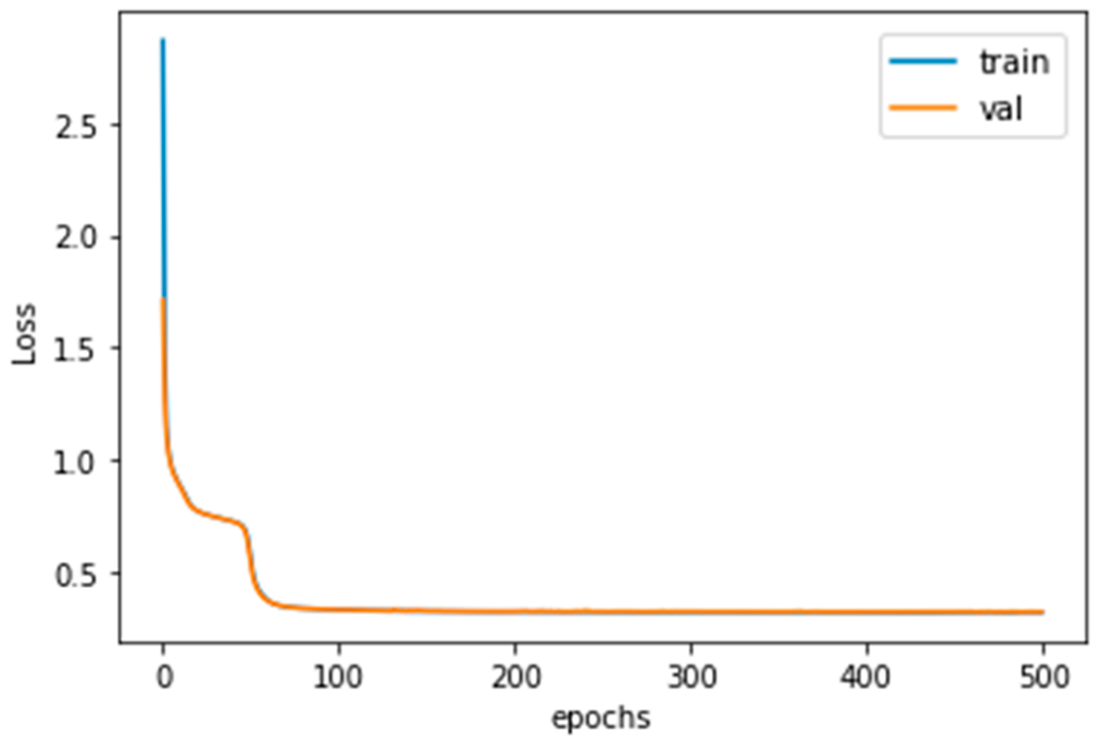
| Learning epochs | 500 |
| Batch learning size | 64 |
| α | 2 |
| β | 1 |
| Performance | Values |
|---|---|
| Train data accuracy | 100.00% |
| Val. data accuracy | 100.00% |
| Test data accuracy | 87.03% |
| Train data loss | 0.318 |
© 2020 by the authors. Licensee MDPI, Basel, Switzerland. This article is an open access article distributed under the terms and conditions of the Creative Commons Attribution (CC BY) license (http://creativecommons.org/licenses/by/4.0/).
Share and Cite
Lo, C.-C.; Lee, C.-H.; Huang, W.-C. Prognosis of Bearing and Gear Wears Using Convolutional Neural Network with Hybrid Loss Function. Sensors 2020, 20, 3539. https://doi.org/10.3390/s20123539
Lo C-C, Lee C-H, Huang W-C. Prognosis of Bearing and Gear Wears Using Convolutional Neural Network with Hybrid Loss Function. Sensors. 2020; 20(12):3539. https://doi.org/10.3390/s20123539
Chicago/Turabian StyleLo, Chang-Cheng, Ching-Hung Lee, and Wen-Cheng Huang. 2020. "Prognosis of Bearing and Gear Wears Using Convolutional Neural Network with Hybrid Loss Function" Sensors 20, no. 12: 3539. https://doi.org/10.3390/s20123539
APA StyleLo, C.-C., Lee, C.-H., & Huang, W.-C. (2020). Prognosis of Bearing and Gear Wears Using Convolutional Neural Network with Hybrid Loss Function. Sensors, 20(12), 3539. https://doi.org/10.3390/s20123539