An Integrated Method for Coding Trees, Measuring Tree Diameter, and Estimating Tree Positions

Abstract

Accurately measuring tree diameter at breast height (DBH) and estimating tree positions in a sample plot are important in tree mensuration. The main aims of this paper include (1) developing a new, integrated device that can identify trees using the quick response (QR) code technique to record tree identifications, measure DBH, and estimate tree positions concurrently; (2) designing an innovative algorithm to measure DBH using only two angle sensors, which is simple and can reduce the impact of eccentric stems on DBH measures; and (3) designing an algorithm to estimate the position of the tree by combining ultra-wide band (UWB) technology and altitude sensors, which is based on the received signal strength indication (RSSI) algorithm and quadrilateral localization algorithm. This novel device was applied to measure ten 10 × 10 m square plots of diversified environments and various tree species to test its accuracy. Before measuring a plot, a coded sticker was fixed at a height of 1.3 m on each individual tree stem, and four UWB module anchors were set up at the four corners of the plot. All individual trees’ DBHs and positions within the plot were then measured. Tree DBH, measured using a tree caliper, and the values of tree positions, measured using tape, angle ruler, and inclinometer, were used as the respective reference values for comparison. Across the plots, the decode rate of QR codes was 100%, with an average response time less than two seconds. The DBH values had a bias of 1.89 mm (1.88% in relative terms) and a root mean square error (RMSE) of 5.38 mm (4.53% in relative terms). The tree positions were accurately estimated; the biases on the x-axis and the y-axis of the tree position were −8.55–14.88 cm and −12.07–24.49 cm, respectively, and the corresponding RMSEs were 12.94–33.96 cm and 17.78–28.43 cm. The average error between the estimated and reference distances was 30.06 cm, with a standard deviation of 13.53 cm. The device is cheap and friendly to use in addition to its high accuracy. Although further studies are needed, our method provides a great alternative to conventional tools for improving the efficiency and accuracy of tree mensuration.

1. Introduction

Diameter at breast height (DBH), measured at a height of 1.3 m on the bole of a tree, is the most commonly measured tree attribute [1,2,3], whether for inventory, management, or research purposes, since many tree and forest attributes [4,5], such as basal area, volume [6], and stand density [7], are derived from DBH measurements [8]. Therefore, developing tools that can measure tree DBH accurately, efficiently, and conveniently is always desirable.

Foresters rely on a variety of conventional dendrometers, such as diameter tapes (D-tapes) and tree calipers, to measure tree DBH. These tools are often based on the geometry of circles; trees are presumed to have circular cross-sections [9], although this is rarely true in reality [10,11]. Most tree stems violate this assumption to some level, either in the form of an oval, an ellipse, or a closed convex [12,13,14,15], resulting in biases (mostly overestimates) in DBH when measured by diameter tapers or tree calipers (which often take one measurement) [16,17]. D-tapes are more commonly used for measuring permanent sample plots because they are perceived as being more consistent for repeated DBH measurements [18], while calipers are often preferred for DBH measurements in temporary plots [19]. In tree mensuration, to reduce the impact of eccentric cross-section of a tree, it is often recommended to measure the major and minor diameters of the tree and obtain the average diameter of the two measurements as the tree DBH, which, in literature, is often used as the reference data for comparison purpose [20]. There are other limits to using a D-tape or caliper to measure tree DBH, such as the manual recording of measurements [16,17], thereby reducing efficiency and increasing mistakes in measurement and data entry [18,19]. Both tools, while relatively reliable, are labor-intensive. Some advanced, electronic measurement devices for DBH measurement [20,21,22,23,24], such as electronic tree-measuring forks and electronic tapes, have been developed. The electronic tapes do not solve the problem of eccentric cross-section, while electronic tree-measuring forks are based on an ultrasonic system [25,26], which can be easily affected by environments [27,28,29]. More recently, some methods for measuring DBH using non-contact methods, including terrestrial laser scanning (TLS) [30,31,32,33,34], mobile phones with time-of-flight (TOF) cameras [4,35,36], and close-range photogrammetry (CRP) [1,22,37], have been proposed. These methods use point clouds to extract data, which are expensive [28] and require high computational capacity of microprocessors, limiting their application in forestry inventory. Other than the method of CRP, estimating tree DBH based on the TLS and TOF methods is still based on the assumption that trees are circular in cross section.

Other than tree size measurements, identifying trees and estimating the positions of the trees in a sample plot are important elements for measuring sampling plots [27,28], and this is particularly true for permanent inventory plots where successive measurements are always needed. Conventionally, foresters either use markers or tags to identify trees. This method, while still widely used, is labor-intensive. The spatial information, i.e., the tree positions, represents important information regarding the stand density, as well as in studies of distance-dependent growth and the dynamics of trees and stands. While tree position information is difficult to obtain, studies have shown that the individual tree positions can be determined using a total station or ultrasonic trilateration technology [25,26]. New developments in integrating DBH measurement and tree position estimation, using non-contact methods such as TLS [30,31,32,33,34], TOF cameras [4,35,36], and CRP [1,22,37], have been reported. However, results of these methods can easily be affected by the stand environments such as stand density, abundance of shrubs and vegetation, and light conditions. They are also time-consuming, labor-intensive, and require complicated procedures in data processing [38]. Therefore, many practical and technical restrictions still exist in applying these methods in forestry inventories.

There is a pressing need to develop an integrated system that can identify trees, measure tree DBH, and estimate tree positions concurrently, accurately, and efficiently in terms of both labor and cost. The recent developments in computer science and electronics make this possible. Quick response (QR) code technology [39] is now widely used due to its characteristics of a high capacity in encoding data, strong damage resistance, and fast decoding [39,40,41,42]. The ultra-wide band (UWB) technology is based on sending and receiving carrier-less radio impulses using extremely accurate timing, and it is particularly suitable for estimating distance and positions [43,44]. This technology has constantly gained interest thanks to its high accuracy (i.e., a typical error of 30 cm or less), making it more attractive than other wireless technologies, such as WiFi, ZigBee, and Bluetooth, which can normally estimate the location with an accuracy of several meters [45,46,47,48]. In this paper, we integrated these technologies into a device to identify trees, measure tree DBH, and estimate tree positions concurrently. The device was applied to measure trees in forest plots of different environments and tree species to evaluate its accuracy and efficiency.

2. Technology and Theory

2.1. Design of the Main Device

The main device and its components can be found in Figure 1, and their attribute descriptions are listed in

Table 1. Descriptive statistics of the device’s components ¹.

Component	Chip Model /Type	Interface Type	Parameter	Function
Microprocessor	STC15W4K56	SPI, I2C, Digital, Serial port, etc.	SRAM: 4 KB; Flash: 56 KB;	Data processing
QR scanner	M800	Serial port	Resolution: 20 mil;	QR scanning
Analog-to-digital sampling module	ADS1115	I2C, Analog	16 bits; 4 channels	AD sampling
UWB module	D-DWM-PG1.7	Serial port	Resolution: 1 cm; Range: 0–50 m	Distance Measurement
Altitude sensor	JY901B	Serial port	Resolution: 1 cm	Altitude Measurement
Bluetooth	HC-06	Serial port	Range: 0–15 m	COMM with upper computer
SD card	microSD	SPI	2 GB	Data storage
Angle sensor	P3014-V1	Analog	Resolution: 0.088°	Angle Measurement
Display	OLED	SPI	128 × 64 pixels	Data display
Keyboard	PVC	Digital	7 keys	Command input
Power management circuit	TP4056, DW01, AMS1117, etc.	Digital, Power	Input: 3.7–4.2 V, 5 V; Output: 3.3 V, 5 V	Power management
Battery	Lithium battery	Power	4000 mAh	Power supply

^1. SPI, serial peripheral interface; I2C, inter-integrated circuit; KB, kilobyte; GB, gigabyte; SRAM, static random-access memory; COMM, communication; V, voltage; mAh, milliampere-hour.

. The device consists of a microprocessor, an analog-to-digital sampling (ADS) module, a QR scanner, a secure digital memory card (SD card), an interface, Bluetooth, a power management circuit, a keyboard interface, an altitude sensor, a display interface, and a UWB module. Note that the angle between the left arm and the middle beam is defined as α₁ and that between the middle beam and right arm as α₂ (Figure 1). The geometric centers of the vertex and middle component are on the same line.

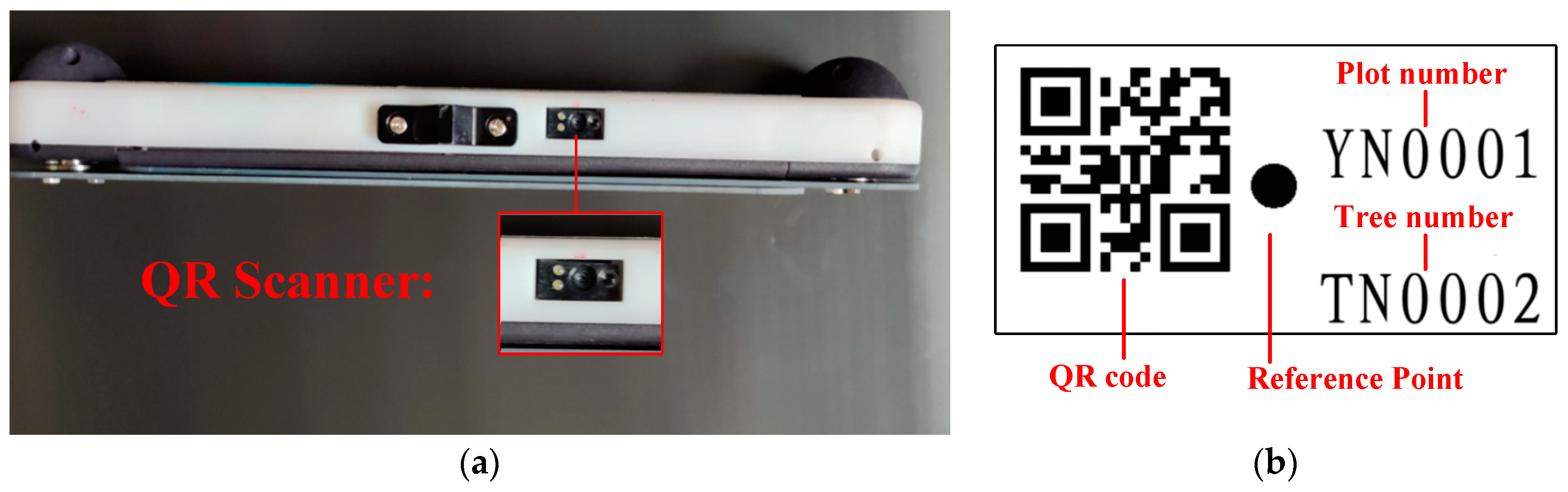
2.2. Technology of Coding Trees

A QR scanner (Figure 2a) is used to decode the QR code (encoded by NiceLabel 2017 Barcode software [19]), which is printed on a sticker (Figure 2b). Other information, such as the identification (ID) numbers of the plot and the tree and the reference point, can also be found on the sticker. For example, for the QR code of “TN0002 | YN0001” (Figure 2b); “TN0002” is the tree ID, and “YN0001” is the sample plot ID. Note that, if stickers are not used, the tree-codes will be generated automatically in the process of measuring trees’ DBH and positions.

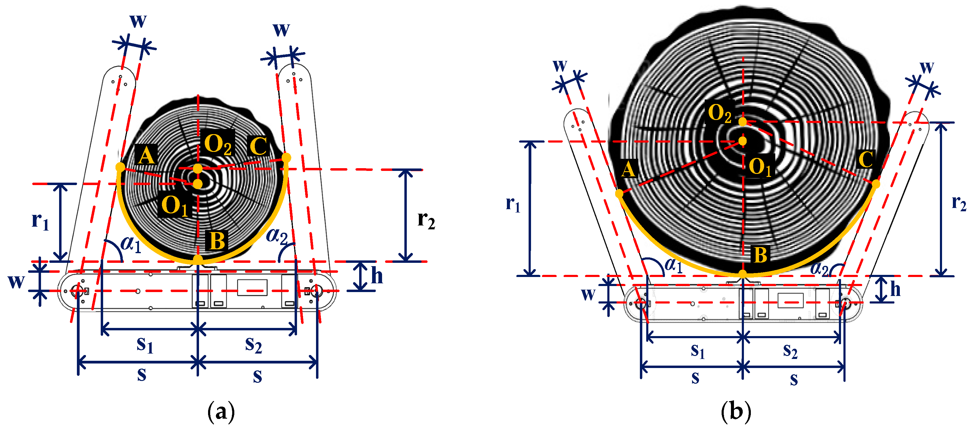
2.3. Angle Calculation

As shown in Figure 1, tree DBH is measured by measuring α_i (i = 1, 2) values. When the central axis of the angle sensor rotates, the change in the angle has a linear relationship with the change in the output voltage signal. Therefore, the voltage signals from ADS modules can be converted to α_i (i = 1, 2) using the following equation:

$${\mathsf{\alpha }}_{\mathrm{i}}=\frac{{360}^{\circ }}{\mathrm{Un}}\times (\mathrm{U}{\mathrm{c}}_{\mathrm{i}}-\mathrm{V}{\mathrm{z}}_{\mathrm{i}}\frac{\mathrm{Un}}{\mathrm{Vr}}),$$

(1)

where U_n is the ADS value of the current input voltage of the two angle sensors, U_ci is the ADS value of the output voltage of the i^th angle sensor, V_zi is the reference value of the output voltage of the i^th angle sensor at initialization when α_i equals 0°, and V_r is the reference value of the input voltage of the two angle sensors at initialization.

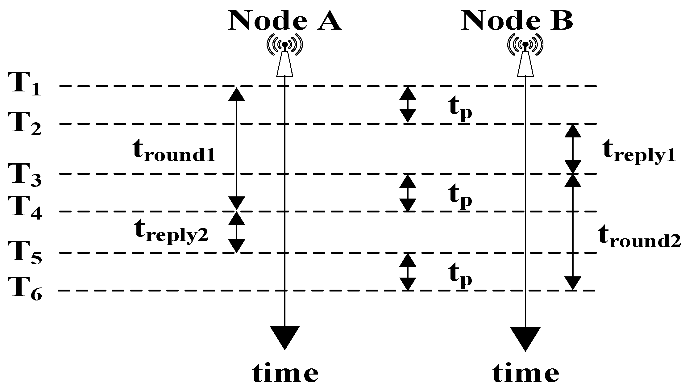
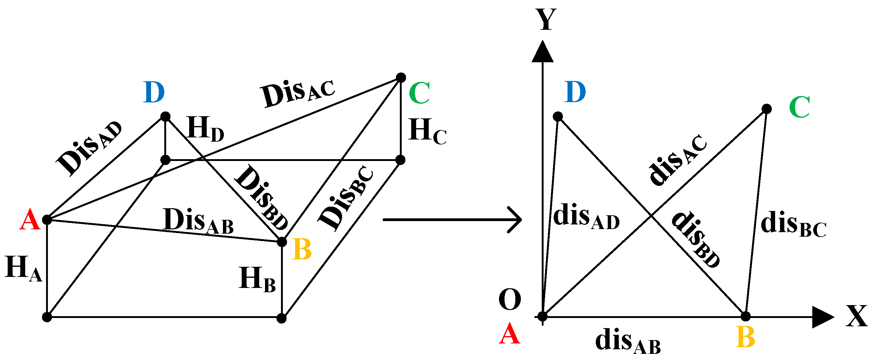
2.4. Double-Sided Two-Way Ranging

The basic ranging principle of the UWB modules used in this method is double-sided two-way ranging (DS-TWR) [46,47,48,49,50]. Clock drift correction and signal power error may affect the accuracy of the position. The DS-TWR is an additional round of communication based on single-sided two-way ranging (SS-TWR) [46,47,48,49,50,51]. The time of the two types of communication can compensate each other for the errors caused by the clock offset [46,47,48,49,50,51,52] and signal power error [51,52] to improve the accuracy of the DS-TWR. Figure 3 presents an example of calculating the distance (Dis) between two nodes (A and B). The distance between node A and node B can be calculated as follows:

$$\mathrm{Dis}=\mathrm{c}\times {\mathrm{t}}_{\mathrm{p}}=\mathrm{c}\times \frac{{\mathrm{t}}_{\mathrm{round1}}\times {\mathrm{t}}_{\mathrm{round2}}-{\mathrm{t}}_{\mathrm{reply1}}\times {\mathrm{t}}_{\mathrm{reply2}}}{{\mathrm{t}}_{\mathrm{round1}}+{\mathrm{t}}_{\mathrm{round2}}+{\mathrm{t}}_{\mathrm{reply1}}+{\mathrm{t}}_{\mathrm{reply2}}},$$

(2)

where node A and node B are two communication UWB nodes; Dis is the distance between node A and node B; t_p is the time of the wireless signal propagation in the air; c is the speed of light in the air; time is the time axis; T₁ is the time when node A sends the first pulse; T₂ is the time when node B receives the first pulse; T₃ is the time when node B sends the first pulse; T₄ is the time when node A receives the first pulse; T₅ is the time when node A sends the second pulse; T₆ is the time when node B receives the second pulse; t_round1 is the total time of node A sending and receiving pulses in the first round of communication; t_reply1 is the reply time for node B in the first round of communication; t_round2 is the total time of node B sending and receiving pulses in the second round of communication; t_reply2 is the reply time for node A in the second round of communication.

3. Materials and Methods

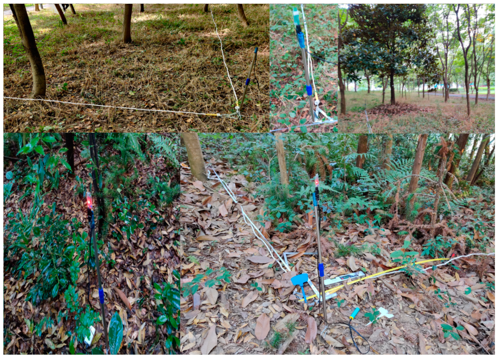
3.1. Study Area

This study was carried out in Lin’an (N30°15′, E119°43′), China. We selected 10 square plots with a size of 10 × 10 m. These plots varied greatly in average tree DBH, environment, and tree species composition (

Table 2. Descriptive statistics of the sample plots ¹.

Plot	Number of Trees	Dominant Species	Slope (°)	DBH (mm)
				Mean	Max	Min	Std
1	16	S1, S2, S3	3.1	140.31	280.32	59.29	61.29
2	19	S1, S4	5.5	136.33	183.91	83.34	28.74
3	15	S1, S5	6.8	144.82	210.24	86.07	32.57
4	18	S2, S3, S6	15.3	153.72	334.63	70.54	75.13
5	28	S1, S3, S6	28.7	125.90	215.37	67.14	49.19
6	37	S7	4.8	102.43	153.97	52.75	30.38
7	30	S7	5.9	112.91	219.90	51.19	40.16
8	24	S2, S3, S7	18.3	179.74	340.21	52.60	88.00
9	20	S3, S7, S8	26.0	118.09	187.99	53.94	39.40
10	18	S7, S9	33.2	127.31	209.57	67.67	45.60

^1. Std, standard deviation; S1, Sapindus mukurossi Gaertn; S2, Cinnamomum camphora; S3, Magnolia denudata; S4, Michelia maudiae Dunn; S5, Ginkgo biloba; S6, Liriodendron chinensis; S7, Cunninghamia lanceolata; S8, Magnolia Grandiflora; S9, Camellia japonica.

). Plots 1–5 were located at the Botanical Garden of Zhejiang A&F University, dominated by artificial forest and turf. Plots 6–10 were located in the suburb of Lin’an, dominated by natural forest, dense weeds, and shrubs.

3.2. Methods

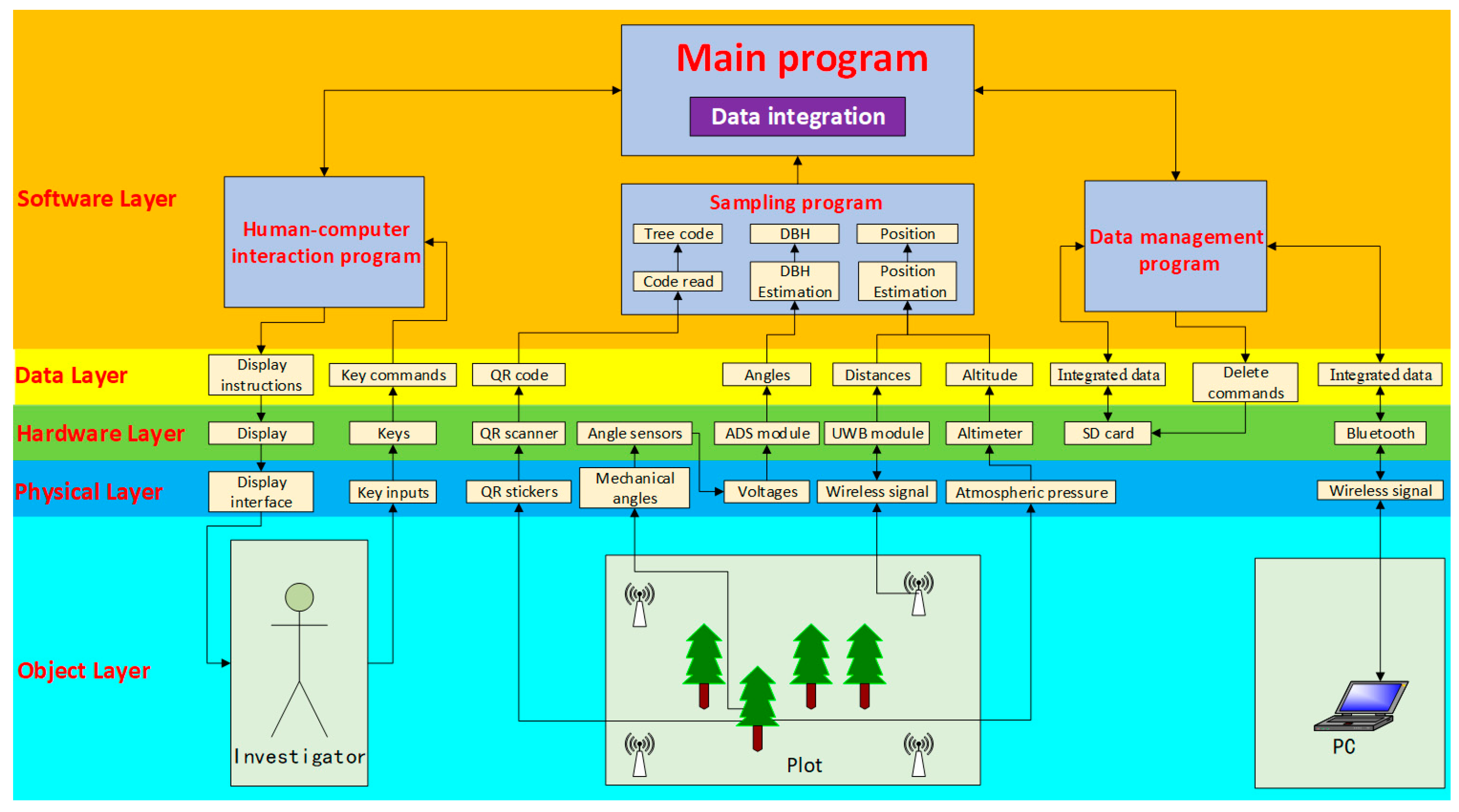
3.2.1. The System Workflow

As shown in Figure 4, the system flow, from top to bottom, consisted of the software layer, data layer, hardware layer, physical layer, and object layer. A few subprograms, including a human–computer interaction program, which is used for keyboard input and display control, a sampling program, which is used for reading tree codes and DBH values and tree position data extraction, and a data management program, which is used for encoding data storage and data communication, were incorporated into the software layer. After completing an individual tree’s measurement (see Section 3.2.2), the tree ID, its DBH value, and position were automatically saved to the system.

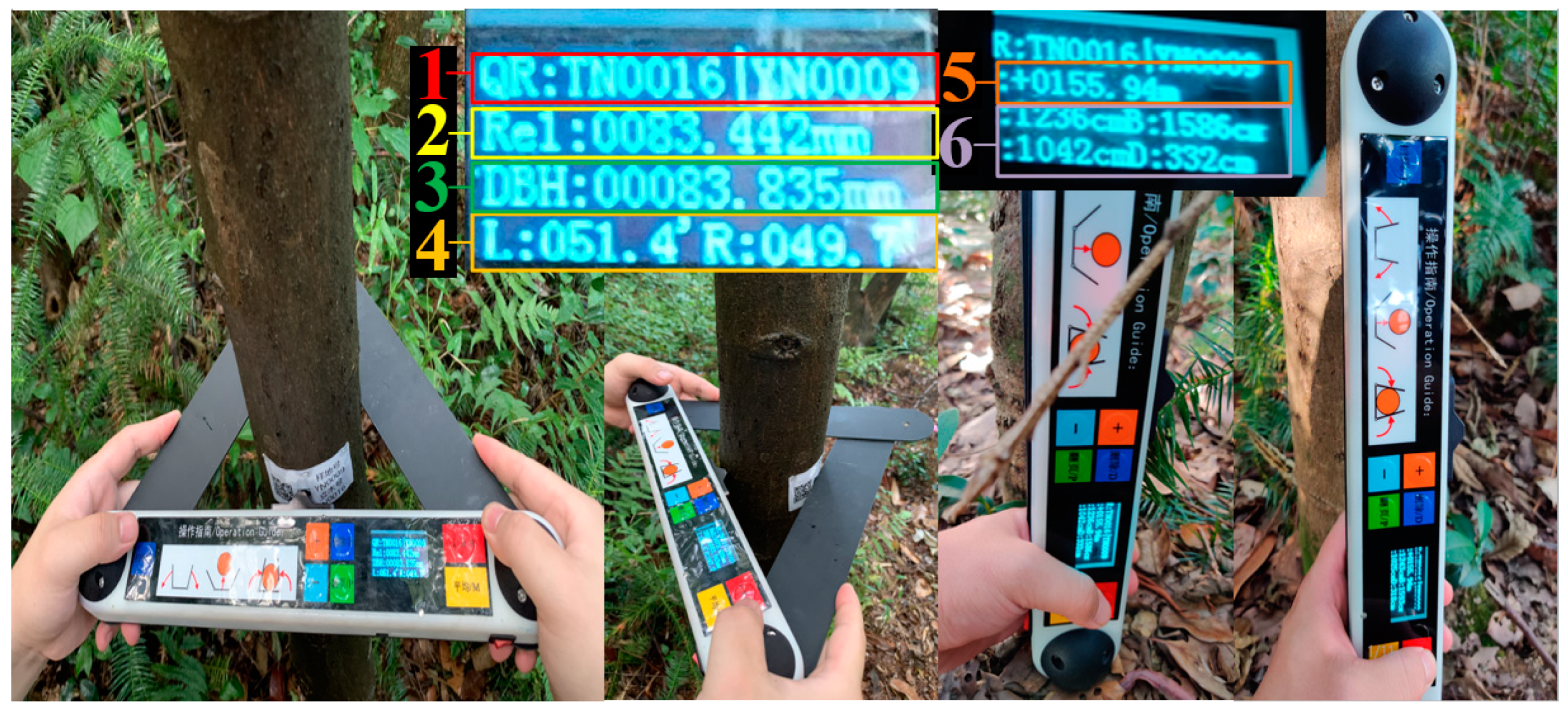
3.2.2. The Operation Workflow

To complete the measurement of a plot, the following tools and instruments are needed: the device, coded stickers, a nail gun, short nails, and four UWB modules (referred to as anchors A, B, C, and D). The coded stickers were fixed at a height of 1.3 m on individual trees in the plot. The anchors (Figure 5 and Figure 6) were set up at plot corners as follows: first, anchor A was set up in one corner of the plot, and then the device was used to measure the altitude of corner A (H_A). Second, anchor B was set up in a neighboring plot corner of A, and the altitude of the corner was measured (H_B) as well as the distance between anchors A and B (Dis_AB). The same step was repeated to set up anchors C and D in the remaining plot corners, and their altitudes (H_C and H_D) were measured as well as the distances between corners (Dis_AC, Dis_BC, Dis_AD, Dis_BD, and Dis_CD).

A tree was measured as follows (Figure 7): first, the investigator scanned the tree QR code, followed by measurement of the tree DBH twice at two different directions (mainly followed the major and minor DBH directions). For each measure, values of α₁ and α₂ were automatically used to calculate the tree DBH (see Section 3.2.3). The average of the two measurements was used as the tree DBH. Finally, the device was placed at the bottom of the tree to obtain H_n, A_n, B_n, C_n, and D_n. Here, H_n is the altitude of the device, A_n, B_n, C_n, or D_n is the distance between anchors A, B, C, or D and the device, respectively, and n refers to the nth tree in the plot. The above steps were repeated to finish measuring all the trees in the plot. Similar to the DBH value, each tree’s position was estimated twice, and the average was used as the tree position value. The measurement data were then uploaded to a person computer (PC) for further analysis.

3.2.3. Measurement Algorithm of a Tree’s DBH

Figure 8 provides an example of measuring tree DBH using the device, with A, B, and C being the contact points of the device’s arms and beam against the tree trunk, which results in two arcs, arc BA and arc BC. Since the cross-section surface may be eccentric, arcs BA and BC have different centers, O₁ and O₂. Note that, for the device, the values of w (2.5 cm), h (3.5 cm), and s (15 cm) are fixed mechanical structural values (Figure 8).

Here, w equals the half width of the arms or beam; h equals w plus the maximum width of the vertex; and s equals the half distance between the axes of two angle sensors.

In order to obtain the value of the tree DBH, the s_i (i = 1,2) values are needed, which can be calculated using Taylor’s expansion in the following equations:

$${\mathrm{s}}_{\mathrm{i}}=\{\begin{array}{ll}\mathrm{s}-\frac{\mathrm{h}\times (1-\frac{{{\mathsf{\theta }}_{\mathrm{i}}}^2}{2!}+\frac{{{\mathsf{\theta }}_{\mathrm{i}}}^4}{4!}-\frac{{{\mathsf{\theta }}_{\mathrm{i}}}^6}{6!})+\mathrm{w}}{{\mathsf{\theta }}_{\mathrm{i}}-\frac{{{\mathsf{\theta }}_{\mathrm{i}}}^3}{3!}+\frac{{{\mathsf{\theta }}_{\mathrm{i}}}^5}{5!}-\frac{{{\mathsf{\theta }}_{\mathrm{i}}}^7}{7!}}\hfill & \left({\mathsf{\alpha }}_{\mathrm{i}}\ne {90}^{\circ }\right)\hfill \\ \mathrm{s}-\mathrm{w}\hfill & \left({\mathsf{\alpha }}_{\mathrm{i}}={90}^{\circ }\right)\hfill \end{array}.$$

(3)

where θ_i = α_i × 3.141592/180 and I = 1, 2.

The calculated s_i can then be used to calculate the radius, r_i, using Taylor’s expansion, in the following equations:

$${\mathrm{r}}_{\mathrm{i}}=\{\begin{array}{ll}{\mathrm{s}}_{\mathrm{i}}\times \frac{\frac{{\mathsf{\theta }}_{\mathrm{i}}}{2}-\frac{{{\mathsf{\theta }}_{\mathrm{i}}}^3}{2^3\times 3!}+\frac{{{\mathsf{\theta }}_{\mathrm{i}}}^5}{2^5\times 5!}-\frac{{{\mathsf{\theta }}_{\mathrm{i}}}^7}{2^7\times 7!}}{1-\frac{{{\mathsf{\theta }}_{\mathrm{i}}}^2}{2^2\times 2!}+\frac{{{\mathsf{\theta }}_{\mathrm{i}}}^4}{2^4\times 4!}-\frac{{{\mathsf{\theta }}_{\mathrm{i}}}^6}{2^6\times 6!}}\hfill & \left({\mathsf{\alpha }}_{\mathrm{i}}\ne {90}^{\circ }\right)\hfill \\ \mathrm{s}-\mathrm{w}\hfill & \left({\mathsf{\alpha }}_{\mathrm{i}}={90}^{\circ }\right)\hfill \end{array}.$$

(4)

The tree DBH is then calculated as the total of r₁ and r₂:

$$\mathrm{DBH}={\mathrm{r}}_1+{\mathrm{r}}_2.$$

(5)

Since r₁ and r₂ are calculated based on different arcs, the impacts of eccentric tree cross-sections on measuring DBH would be accounted for, resulting in a more accurate estimate than that obtained using conventional dendrometers.

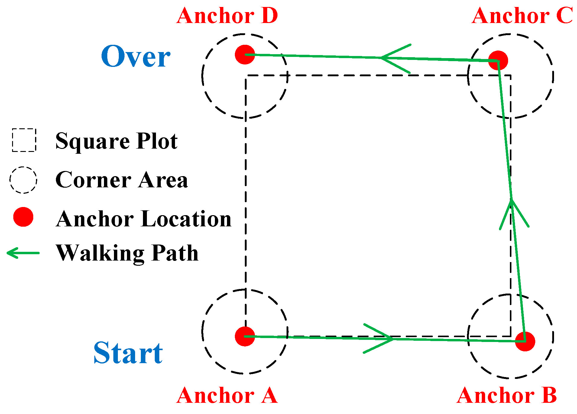
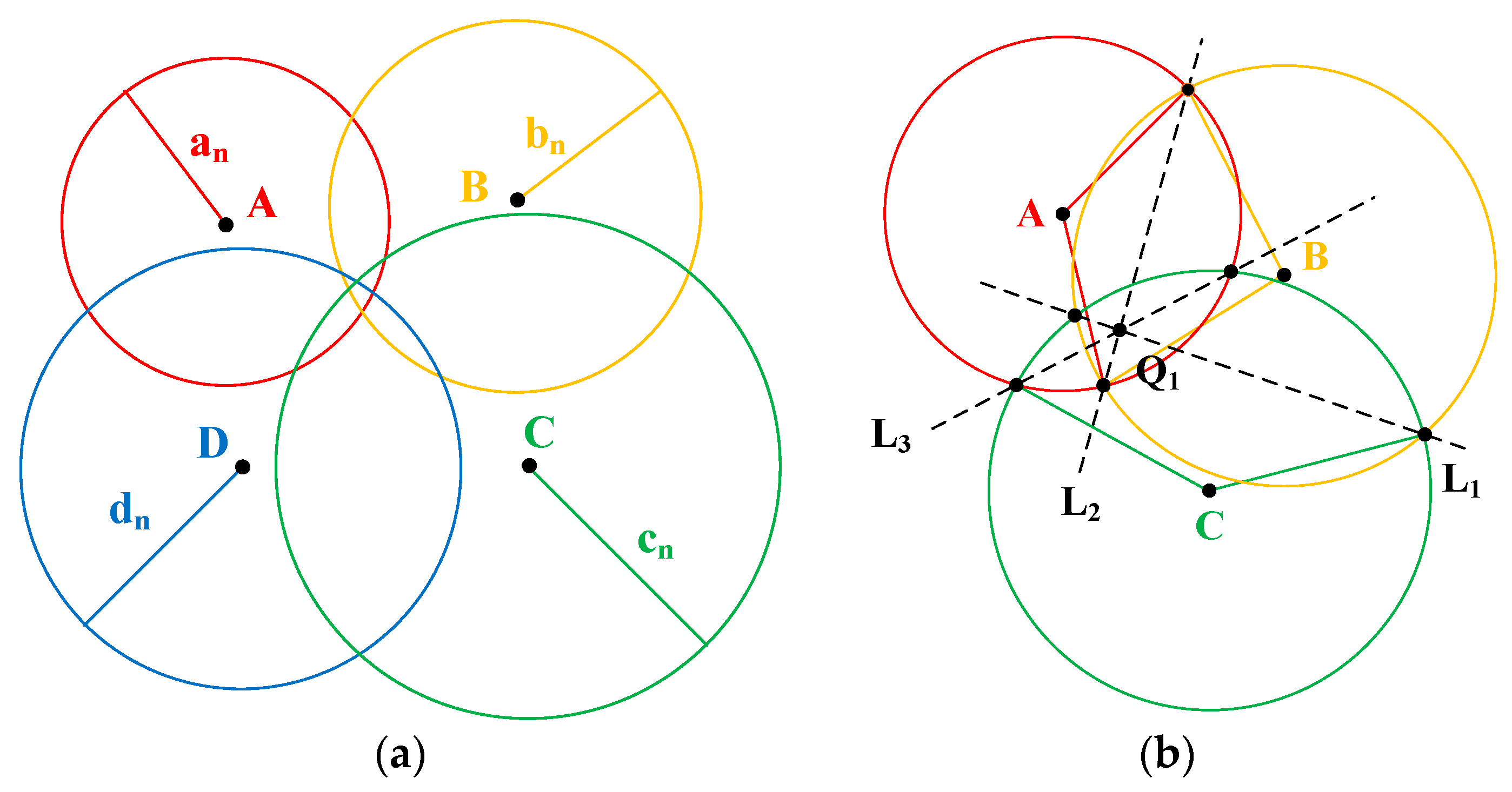
3.2.4. Estimation Algorithm of a Tree Position

In order to obtain a tree’s position in a plot, the spatial coordinate system of four anchors is first transformed into a plane rectangular coordinate system OXY (Figure 9).

The plane OXY is perpendicular to the gravity direction, the origin O is the location of anchor A, and the x-axis is the projection direction from anchor A to anchor B. The three-dimensional scalars H_A, H_B, H_C, H_D, Dis_AB, Dis_BC, Dis_AC, Dis_AD, and Dis_BD are then transformed into two-dimensional scalars in the OXY plane.

$$\begin{array}{l}{\mathrm{dis}}_{\mathrm{AB}}=\sqrt{{{\mathrm{Dis}}_{\mathrm{AB}}}^2{-({\mathrm{H}}_{\mathrm{A}}-{\mathrm{H}}_{\mathrm{B}})}^2}\\ {\mathrm{dis}}_{\mathrm{BC}}=\sqrt{{{\mathrm{Dis}}_{\mathrm{BC}}}^2{-({\mathrm{H}}_{\mathrm{B}}-{\mathrm{H}}_{\mathrm{C}})}^2}\\ {\mathrm{dis}}_{\mathrm{AC}}=\sqrt{{{\mathrm{Dis}}_{\mathrm{AC}}}^2{-({\mathrm{H}}_{\mathrm{A}}-{\mathrm{H}}_{\mathrm{C}})}^2}\\ {\mathrm{dis}}_{\mathrm{AD}}=\sqrt{{{\mathrm{Dis}}_{\mathrm{AD}}}^2{-({\mathrm{H}}_{\mathrm{A}}-{\mathrm{H}}_{\mathrm{D}})}^2}\\ {\mathrm{dis}}_{\mathrm{BD}}=\sqrt{{{\mathrm{Dis}}_{\mathrm{BD}}}^2{-({\mathrm{H}}_{\mathrm{B}}-{\mathrm{H}}_{\mathrm{D}})}^2}\end{array}$$

(6)

The coordinates of anchors A, B, C, and D can then be obtained.

$$\begin{array}{l}\left({\mathrm{X}}_{\mathrm{A}},{\mathrm{Y}}_{\mathrm{A}}\right)=(0,0)\\ \left({\mathrm{X}}_{\mathrm{B}},{\mathrm{Y}}_{\mathrm{B}}\right)=(0,{\mathrm{dis}}_{\mathrm{AB}})\\ ({\mathrm{X}}_{\mathrm{C}},{\mathrm{Y}}_{\mathrm{C}})=(\frac{{{\mathrm{dis}}_{\mathrm{AB}}}^2+{{\mathrm{dis}}_{\mathrm{AC}}}^2-{{\mathrm{dis}}_{\mathrm{BC}}}^2}{2{\mathrm{dis}}_{\mathrm{AB}}},\sqrt{{{\mathrm{dis}}_{\mathrm{AC}}}^2-{(\frac{{{\mathrm{dis}}_{\mathrm{AB}}}^2+{{\mathrm{dis}}_{\mathrm{AC}}}^2-{{\mathrm{dis}}_{\mathrm{BC}}}^2}{2{\mathrm{dis}}_{\mathrm{AB}}})}^2})\\ ({\mathrm{X}}_{\mathrm{D}},{\mathrm{Y}}_{\mathrm{D}})=(\frac{{{\mathrm{dis}}_{\mathrm{AB}}}^2+{{\mathrm{dis}}_{\mathrm{AD}}}^2-{{\mathrm{dis}}_{\mathrm{BD}}}^2}{2{\mathrm{dis}}_{\mathrm{AB}}},\sqrt{{\mathrm{disAD}}^2-{(\frac{{{\mathrm{dis}}_{\mathrm{AB}}}^2+{{\mathrm{dis}}_{\mathrm{AD}}}^2-{{\mathrm{dis}}_{\mathrm{BD}}}^2}{2{\mathrm{dis}}_{\mathrm{AB}}})}^2})\end{array}$$

(7)

Similarly, the projection distances a_n, b_n, c_n, and d_n can be calculated as follows:

$$\begin{array}{l}{\mathrm{a}}_{\mathrm{n}}=\sqrt{{{\mathrm{A}}_{\mathrm{n}}}^2{-({\mathrm{H}}_{\mathrm{A}}-{\mathrm{H}}_{\mathrm{n}})}^2}\\ {\mathrm{b}}_{\mathrm{n}}=\sqrt{{{\mathrm{B}}_{\mathrm{n}}}^2{-({\mathrm{H}}_{\mathrm{B}}-{\mathrm{H}}_{\mathrm{n}})}^2}\\ {\mathrm{c}}_{\mathrm{n}}=\sqrt{{{\mathrm{C}}_{\mathrm{n}}}^2{-({\mathrm{H}}_{\mathrm{C}}-{\mathrm{H}}_{\mathrm{n}})}^2}\\ {\mathrm{d}}_{\mathrm{n}}=\sqrt{{{\mathrm{D}}_{\mathrm{n}}}^2{-({\mathrm{H}}_{\mathrm{D}}-{\mathrm{H}}_{\mathrm{n}})}^2}\end{array}$$

(8)

Here, a_n, b_n, c_n, and d_n represent the projection distances between anchors A, B, C, and D, respectively, and the device in the OXY plane. n refers to the nth tree in the plot.

Although UWB wireless signals have very strong penetration ability, in reality, the random ranging error may be caused by humans and/or the tree body [48,49,50,51,52,53], resulting in a prolonged communication time between the UWB nodes. Therefore, the values of a_n, b_n, c_n, and d_n may be slightly higher than the respective actual values, and consequently, the four circles may not intersect at one common point (Figure 10a). The received signal strength indication (RSSI) algorithm [50,51,52,53,54,55,56], such as quadrilateral localization (Figure 10a), provides an alternative to solve this problem and to improve the accuracy and precision.

From Figure 10a, we can develop four trilateration localizations with each of three circles (ABC, ABD, ACD, and BCD). Taking ABC (Figure 10b) as an example, where three circles, A, B, and C are intersected, three lines, L₁, L_2, and L₃, are formed by linking the intersections of any two circles. According to the trilateration localization algorithm [53,54,55,56,57,58], the following equations can be developed:

$$\{\begin{array}{l}2({\mathrm{X}}_{\mathrm{A}}-{\mathrm{X}}_{\mathrm{B}}){\mathrm{X}}_1+2({\mathrm{Y}}_{\mathrm{A}}-{\mathrm{Y}}_{\mathrm{B}}){\mathrm{Y}}_1={{\mathrm{b}}_{\mathrm{n}}}^2-{{\mathrm{a}}_{\mathrm{n}}}^2+{{\mathrm{X}}_{\mathrm{A}}}^2-{{\mathrm{X}}_{\mathrm{B}}}^2+{{\mathrm{Y}}_{\mathrm{A}}}^2-{{\mathrm{Y}}_{\mathrm{B}}}^2\\ 2({\mathrm{X}}_{\mathrm{B}}-{\mathrm{X}}_{\mathrm{C}}){\mathrm{X}}_1+2({\mathrm{Y}}_{\mathrm{B}}-{\mathrm{Y}}_{\mathrm{C}}){\mathrm{Y}}_1={{\mathrm{c}}_{\mathrm{n}}}^2-{{\mathrm{b}}_{\mathrm{n}}}^2+{{\mathrm{X}}_{\mathrm{B}}}^2-{{\mathrm{X}}_{\mathrm{C}}}^2+{{\mathrm{Y}}_{\mathrm{B}}}^2-{{\mathrm{Y}}_{\mathrm{C}}}^2\\ 2({\mathrm{X}}_{\mathrm{A}}-{\mathrm{X}}_{\mathrm{C}}){\mathrm{X}}_1+2({\mathrm{Y}}_{\mathrm{A}}-{\mathrm{Y}}_{\mathrm{C}}){\mathrm{Y}}_1={{\mathrm{c}}_{\mathrm{n}}}^2-{{\mathrm{a}}_{\mathrm{n}}}^2+{{\mathrm{X}}_{\mathrm{A}}}^2-{{\mathrm{X}}_{\mathrm{C}}}^2+{{\mathrm{Y}}_{\mathrm{A}}}^2-{{\mathrm{Y}}_{\mathrm{C}}}^2\end{array}.$$

(9)

The coordinates of Q₁ (X₁, Y₁) can be obtained from Equation (9). By the same token, the coordinates of the three other connecting points of the three other trilateration localizations can be obtained—Q₂ (X₂,Y₂), Q₃ (X₃,Y₃), and Q₄ (X₄,Y₄). Then, according to the RSSI algorithm and quadrilateral localization algorithm [59], the above equations can be used to calculate the coordinates of X_n and Y_n as follows:

$$\{\begin{array}{c}{\mathrm{X}}_{\mathrm{n}}=\frac{\frac{{\mathrm{X}}_1}{{\mathrm{a}}_{\mathrm{n}}+{\mathrm{b}}_{\mathrm{n}}+{\mathrm{c}}_{\mathrm{n}}}+\frac{{\mathrm{X}}_2}{{\mathrm{a}}_{\mathrm{n}}+{\mathrm{b}}_{\mathrm{n}}+{\mathrm{d}}_{\mathrm{n}}}+\frac{{\mathrm{X}}_3}{{\mathrm{a}}_{\mathrm{n}}+{\mathrm{c}}_{\mathrm{n}}+{\mathrm{d}}_{\mathrm{n}}}+\frac{{\mathrm{X}}_4}{{\mathrm{b}}_{\mathrm{n}}+{\mathrm{c}}_{\mathrm{n}}+{\mathrm{d}}_{\mathrm{n}}}}{\frac{1}{{\mathrm{a}}_{\mathrm{n}}+{\mathrm{b}}_{\mathrm{n}}+{\mathrm{c}}_{\mathrm{n}}}+\frac{1}{{\mathrm{a}}_{\mathrm{n}}+{\mathrm{b}}_{\mathrm{n}}+{\mathrm{d}}_{\mathrm{n}}}+\frac{1}{{\mathrm{a}}_{\mathrm{n}}+{\mathrm{c}}_{\mathrm{n}}+{\mathrm{d}}_{\mathrm{n}}}+\frac{1}{{\mathrm{b}}_{\mathrm{n}}+{\mathrm{c}}_{\mathrm{n}}+{\mathrm{d}}_{\mathrm{n}}}}\\ {\mathrm{Y}}_{\mathrm{n}}=\frac{\frac{\mathrm{Y}1}{{\mathrm{a}}_{\mathrm{n}}+{\mathrm{b}}_{\mathrm{n}}+{\mathrm{c}}_{\mathrm{n}}}+\frac{\mathrm{Y}2}{{\mathrm{a}}_{\mathrm{n}}+{\mathrm{b}}_{\mathrm{n}}+{\mathrm{d}}_{\mathrm{n}}}+\frac{\mathrm{Y}3}{{\mathrm{a}}_{\mathrm{n}}+{\mathrm{c}}_{\mathrm{n}}+{\mathrm{d}}_{\mathrm{n}}}+\frac{\mathrm{Y}4}{{\mathrm{b}}_{\mathrm{n}}+{\mathrm{c}}_{\mathrm{n}}+{\mathrm{d}}_{\mathrm{n}}}}{\frac{1}{{\mathrm{a}}_{\mathrm{n}}+{\mathrm{b}}_{\mathrm{n}}+{\mathrm{c}}_{\mathrm{n}}}+\frac{1}{{\mathrm{a}}_{\mathrm{n}}+{\mathrm{b}}_{\mathrm{n}}+{\mathrm{d}}_{\mathrm{n}}}+\frac{1}{{\mathrm{a}}_{\mathrm{n}}+{\mathrm{c}}_{\mathrm{n}}+{\mathrm{d}}_{\mathrm{n}}}+\frac{1}{{\mathrm{b}}_{\mathrm{n}}+{\mathrm{c}}_{\mathrm{n}}+{\mathrm{d}}_{\mathrm{n}}}}\end{array}.$$

(10)

3.2.5. Evaluation of the Accuracy of the DBH and Tree Position

The major and minor DBHs of each tree were measured using a caliper in the 10 plots, and their average was used as the reference DBH value for comparison. The accuracy of using the device to measure tree DBH was evaluated by comparison with the reference DBH values and by calculating the error, bias, relative bias, root mean square error (RMSE), relative RMSE, and mean absolute percent error (MAPE), as defined in the following equations:

$$\mathrm{error}={\mathrm{d}}_j-{\mathrm{d}}_{j\mathrm{r}},$$

(11)

$$\mathrm{BIAS}=\frac{{\displaystyle {\sum }_{j=1}^n({\mathrm{d}}_j-{\mathrm{d}}_{j\mathrm{r}})}}{n},$$

(12)

$$\mathrm{relBIAS}=\frac{{\displaystyle {\sum }_{j=1}^n({\mathrm{d}}_j/{\mathrm{d}}_{jr}-1)}}{n}\times 100\%,$$

(13)

$$\mathrm{RMSE}=\sqrt{\frac{{\displaystyle {\sum }_{j=1}^n{({\mathrm{d}}_j-{\mathrm{d}}_{jr})}^2}}{n}},$$

(14)

$$\mathrm{relRMSE}=\sqrt{\frac{{\displaystyle {\sum }_{j=1}^n{({\mathrm{d}}_j/{\mathrm{d}}_{jr}-1)}^2}}{n}}\times 100\%,$$

(15)

$$\mathrm{MAPE}=\frac{{\displaystyle {\sum }_{j=1}^n\left|({\mathrm{d}}_j/{\mathrm{d}}_{jr}-1)\right|}}{n}\times 100\%,$$

(16)

where d_j is the jth tree DBH measured using the device, d_jr is the jth tree reference DBH measured using the caliper, and n is the number of measured trees.

The reference value of the tree position was also measured and converted into the OXY plane coordinate system. First, the plane coordinate of the tree bottom position nearest to the x-axis or y-axis was determined by the measured values of a tape scale, an angle ruler, and an inclinometer. Then, half of the tree DBH value was added to or subtracted from the reference position value of the plane coordinate in the y-axis or x-axis direction. The BIAS and RMSE were calculated to reflect the accuracy of the tree position in the x-axis and y-axis directions, respectively. The errors of the distance (Ed) between the estimated and the reference position values were calculated as follows:

$$\mathrm{Ed}=\sqrt{{({\mathrm{X}}_j-{\mathrm{X}}_{jr})}^2+{({\mathrm{Y}}_j-{\mathrm{Y}}_{jr})}^2}.$$

(17)

Here, x_j and y_j are the jth tree position estimators in the x- and y-axis directions, respectively; x_jr and y_jr are the jth position reference values in the x- and y-axis directions, respectively, of the OXY plane coordinate system.

4. Results

4.1. Tree Identification

The decoding rate of QR codes from the coded stickers on trees was 100%, and the decoding response time was short, less than two seconds.

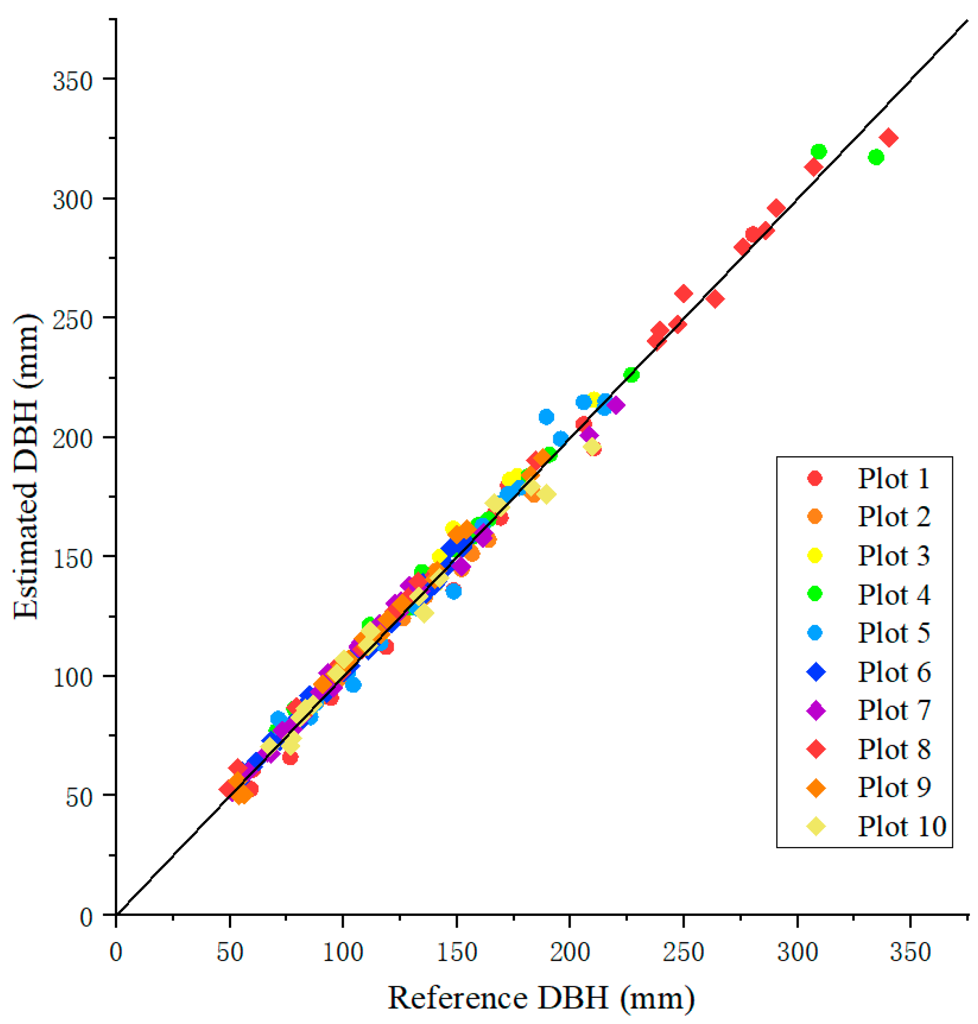
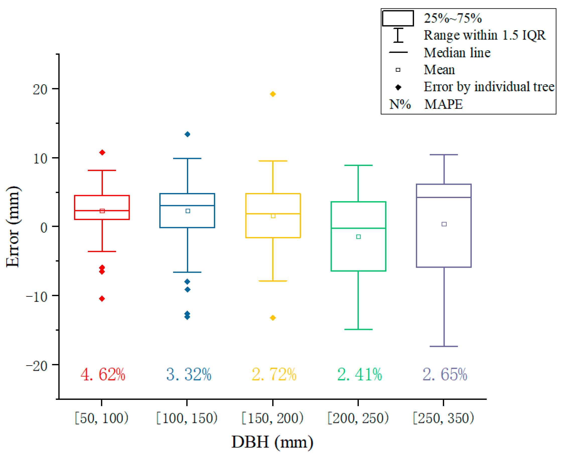
4.2. Evaluation of DBH

The DBHs measured by the device were similar to those measured by the caliper (Figure 11), resulting in an overall BIAS of 1.89 mm (1.88%) and an RMSE of 5.38 mm (4.53%) across all plots (

Table 3. Accuracy of DBHs measured by the device based on a comparison with the reference DBHs measured by a caliper.

Plot	BIAS (mm)	relBIAS (%)	RMSE (mm)	relRMSE (%)
					1	−2.04	−2.04	6.65	5.76
2	−1.22	−0.64	3.52	2.29
3	5.13	3.50	6.44	4.43
4	3.34	3.54	6.84	5.27
5	1.87	1.85	5.94	5.01
6	2.40	2.65	3.48	3.85
7	2.33	2.53	4.79	4.11
8	3.33	3.17	5.93	4.96
9	3.25	2.41	4.72	4.77
10	−0.62	−0.25	6.42	4.76
Total	1.89	1.88	5.38	4.53

). The BIAS for an individual plot varied from −0.62 (Plot 10) to 5.13 mm (Plot 3), and on a relative term from −0.25 to 3.54%. The RMSE values by plot were small, ranging from 3.48 to 6.84 mm, and from 2.29 to 5.76% in a relative term. Variation in BIAS or RMSE was not strongly related to tree DBH size, tree species, and plot slope (Table 3). Also, the BIAS or RMSE between the plots in the botanical garden (plots 1–5) and those in the natural stands (plots 6–10) were comparable. The error for each tree size distributed normally (Figure 12). There was a trend, however, that as the DBH increased, more variation in error was observed. The smaller DBH groups tended to have larger MAPEs. For the largest DBH group (from 250 to 350 mm), the average error was larger than zero, suggesting that the device overestimated the tree DBH compared to the caliper.

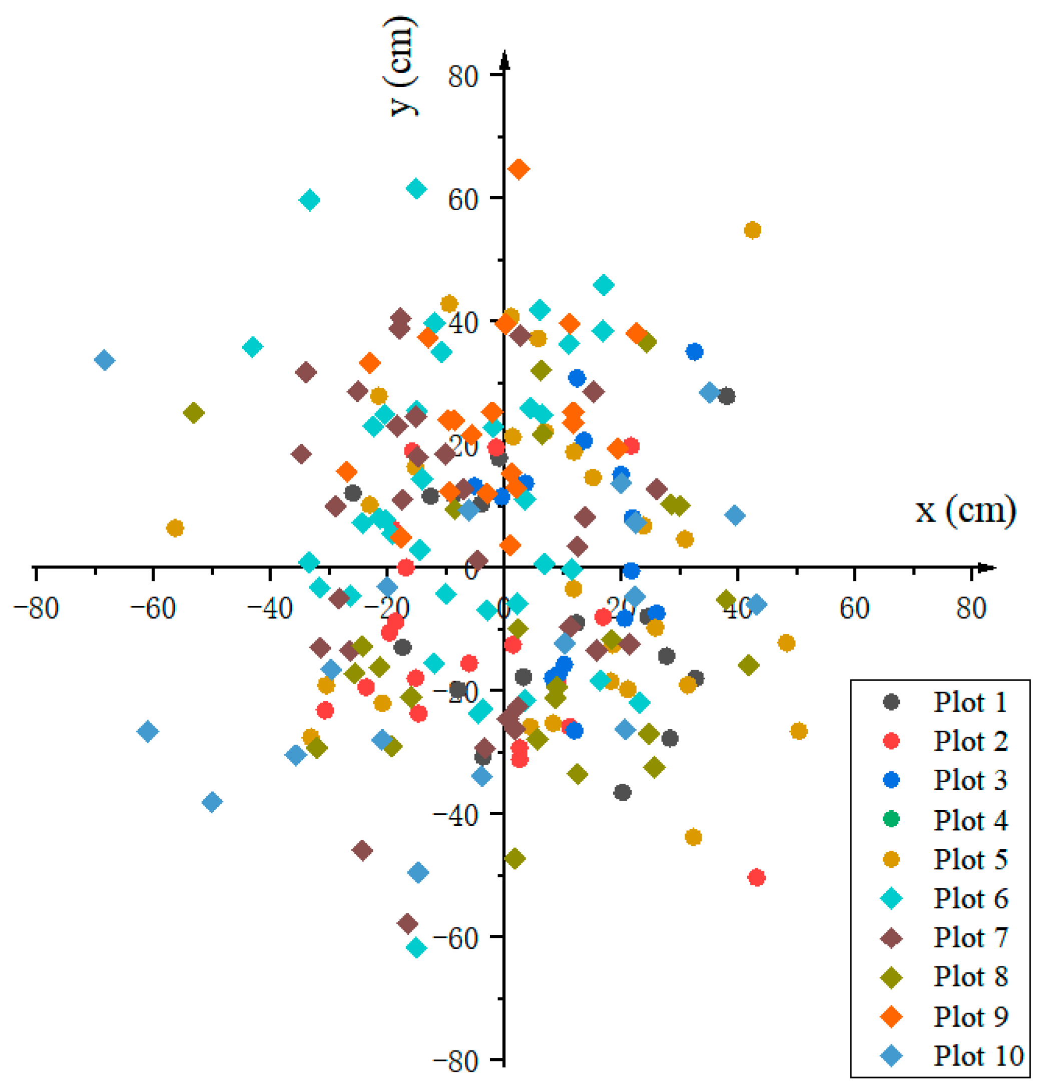
4.3. Evaluation of Tree Position

Figure 13 presents the errors of the distance (Ed) between the estimated and corresponding reference position values by individual tree, ranging from 0 to 77 cm in the plane OXY. The bias ranged from approximately −8.55 to 14.88 cm on the x-axis and from −12.07 cm to 24.69 cm on the y-axis (

Table 4. Accuracy of tree positions in the x- and y-axis directions estimated by the device.

Plot	X (cm)		Y (cm)		ρxy
	BIAS	RMSE	BIAS	RMSE
1	6.51	20.21	−6.40	19.72	−0.22
2	−3.97	18.45	−12.07	21.73	−0.26
3	13.65	16.82	3.67	18.44	0.13
4	0.26	23.54	−3.86	23.06	−0.21
5	14.88	26.59	−3.75	25.17	−0.12
6	−8.19	18.05	10.58	27.94	−0.09
7	−8.55	19.37	3.19	25.12	−0.11
8	3.36	23.93	−9.57	24.03	0.04
9	−1.89	12.94	24.69	28.43	0.23
10	−5.50	33.96	−9.63	24.71	0.30
Total	−0.80	21.91	1.21	24.62	−0.07

). The RMSEs in the x-axis (21.85 cm) and y-axis (24.53 cm) directions were similar (Table 4). No significant correlation (approximately −0.26 to 0.30) was found between the errors in the x-axis and y-axis directions. The mean value of Ed was 30.06 cm, with a standard deviation of 13.53 cm across plots and ranged from 23.44 to 38.08 cm by plot (

Table 5. Summary statistics of the error of the distance (Ed) between the estimated point and the reference point.

Plot	Ed (cm)
	Mean	Max	Min	Std
1	26.21	47.10	11.20	10.84
2	26.19	66.18	12.56	11.25
3	23.44	47.84	11.58	8.88
4	30.84	58.23	10.85	11.61
5	33.98	69.34	12.18	13.26
6	29.42	68.47	6.18	15.53
7	29.37	60.12	4.78	11.96
8	31.99	58.87	10.05	10.77
9	28.00	64.92	3.84	13.36
10	38.08	76.40	11.27	16.99
Total	38.06	76.40	3.84	13.53

). The average Ed of plots 1 to 5 was relatively lower than that of plots 6 to 10. Additionally, if the plot had a larger slope or more trees, Ed was relatively larger. Across all plots, the correlation coefficients of the mean Ed were 0.78 with the slope and 0.24 with the stand density. Relatively, slope had relatively more influence on mean Ed than the stand density.

5. Discussion

In this study, we reported a device that can identify trees using QR code technology, measure tree DBHs using angle sensors, and estimate tree positions using UWB modules and altitude sensors. Use of the QR code is very common in modern daily life, due to its low cost and advanced technology, but it is rarely used in forestry, especially in inventory plot surveys. To our knowledge, this is the first study to integrate QR code technology into a tree dendrometer to identify trees. In forestry inventories, tree identification data are of high value for retrospective data and database management development.

Conventional dendrometers are only accurate for trees that are circular in cross-section. When a tree cross-section is eccentric, it is recommended to measure the major and minor diameters or two diameters perpendicular to each other, using a tree caliper, and to use their average as the tree DBH value [26]. Different from conventional tools, the device described here takes into account the fact that the cross-sections of trees are not always circular by calculating the radii of different arcs. We evaluated the accuracy of the device in measuring DBH by comparing it to the corresponding DBH values measured twice using a tree caliper. The resulting BIAS and RMSE were small (Table 3), suggesting the device is accurate in measuring tree DBH. Modern tools to measure DBH have been developed to improve accuracy. Liang et al. [8] used a multi-single-scan TLS method to estimate tree DBH. Those authors mapped five dense forest plots, compared the results with manual field measurements, and reported an RMSE range from 0.90 to 1.90 cm. Reference [4] estimated the tree DBH of nine square plots using simultaneous localization and mapping (SLAM) algorithms paired with a time-of-flight (TOF) camera. The DBH estimations had a 0.33 mm (1.78%) BIAS and a 1.26 cm (6.39%) RMSE. Reference [1] used unmanned aerial system-based photogrammetry and terrestrial photogrammetry to estimate tree DBH. The error of the diameter estimation was observed to be less than 1 cm in terms of RMSE. Reference [27] used 3D point clouds of individual trees collected using the CRP method to estimate the tree DBH of four species. The relative RMSE varied from 0.90% to 1.85%, strongly depending on tree species. While the accuracies of the above methods are high and time-efficient, their practical applications in forest inventories, particular in large and dense forests, are still limited since these methods involve complicated procedures in data processing and require specific tools. Even though our method is based on a simple trigonometric theorem, the obtained BIAS (0.19 cm and 1.88%) and RMSE (0.54 cm and 4.53%) (Table 3) were either comparable to or even lower than those reported above. The DBH measurement accuracy of the methods based on TLS, CRP, or TOF may be affected by environmental conditions such as light intensity and stand density. The effects of environmental conditions on our device’s accuracy may be small, which explains why the BIAS and RMSE (Table 3) did not vary substantially with plot slope, tree species, or stand type.

Our results also suggest that the device can estimate tree positions accurately, with the resulting BIAS (−8.55 to 14.88 cm on the x-axis and −12.07 to 24.49 cm on the y-axis), RMSE (12.94–33.96 cm and 17.78–28.43 cm on the x-axis and the y-axis, respectively), and Ed (30.06 cm) being small. Reference [4] estimated the tree position using the SLAM algorithms paired with a TOF camera and reported an RMSE of 0.12 m, regardless of the axis directions. Their results, however, were based on sample plots on a flat site with no weeds and small shrubs; therefore, the actual use of their method in dense forests needs further verification. While application of SLAM algorithms paired with a TOF seems promising in terms of precision, it is known to be affected by stand environments, such as stand density, abundance of shrubs and vegetation, etc., and involves complicated data processing procedures, limiting its application to forest inventory. Reference [37] reported a position error of less than 0.5 m, although with a systematic shift, and they used five cameras to realize their method, which is impractical for forest surveys. Reference [44] used an extended Kalman filter (EKF) method that integrated inertial navigation system (INS) and UWB data. They tested their method in an indoor area of 10 × 10 m and found that the positioning error of UWB was between 10 and 30 cm and INS-UWB was less than 15 cm. Clearly, our device can obtain similar or more accurate position estimates than the above cited methods, even our device only uses the trilateration localization algorithm, RSSI algorithm, and quadrilateral localization algorithm, which have a much lower complexity in both time and space. Note that the accuracy in estimating tree positions using our device may be affected by stand environments. The slope correlated more positively with Ed than the stand density did (Table 2 and Figure 14). Therefore, further studies are needed to improve accuracy in estimating positions in various environments and find how to reduce influence from slope.

Note that the plot size adopted in this study is 100 m², much smaller than the regular plot size often used in forestry inventory. This raises a concern of using the device to estimate positions in more realistic scenarios since the performance of four UWB sensors would probably degrade when the plot area is large. However, the range accuracy deteriorates only when the distance between two UWB nodes is over 100 m [59], which is much longer than the side length of a typical plot. In a plot of regular size, the line-of-sight (LOS) paths between nodes may be obstructed, resulting in None-Line-of-Sight (NLOS) situations, in particular when the plot is located within a natural, dense stand. Even the UWB technology offers the great potential of achieving high ranging accuracy through its ability to resolve multipath and penetrate obstacles in harsh environments [60], its localization performance may be reduced by NLOS propagation. Although UWB signal cannot penetrate metal media or thick wall, it does have capability of penetrating trees or weed, which was supported by measuring some of the plots in this study where NLOS were true. Furthermore, several techniques have been proposed to reduce the impact of NLOS range estimates on the estimated agent position [60]. Conventionally, the RSSI is not popularly used for UWB because it does not exploit fine space resolution of impulsive signals [61]. In our method, at least three points are required in order to calculate the position on the plane, which fitted well for RSSI algorithm and four UWB Anchors. In every calculation, we need to deal with four positions (Q₁ (X₁, Y₁), Q₂ (X₂, Y₂), Q₃ (X₃, Y₃), and Q₄ (X₄, Y₄)) obtained from four tri-UWB Anchors combinations. If one position has a stronger signal, it will be given more weight (see Equation (10)). Overall, extension of the results to typical large plots, in particular when they are located in dense stands, should be taken with caution and further studies on this topic should be carried out to confirm our findings. Alternatively, measurements can be done based on four sensors for every 10 m × 10 m area. This seems feasible, at least economically, since each UWB sensor costs less than twenty dollars.

The SLAM algorithm, convex hull algorithm, and point cloud algorithm used in other studies [4,25,27,37] usually need mobile phones or computers with 32- or 64-bit capacity. The device reported in this paper only needs the STC15, an 8-bit microprocessor, with the price being less than one dollar. In terms of computation, our method only needs four operations to obtain the estimates of DBH and tree position, making it much simpler than the other algorithm-based methods.

6. Conclusions

The novelty of the dendrometer reported here is that the device can measure tree identification, position, and DBH concurrently. Specifically, we integrated several advanced technologies (UWB, QR code, altitude sensor, and so on) into the device to improve the measurement accuracy. The experimental results show that this device can be used to accurately estimate DBH and tree positions. Additionally, the device is cheap and easy to use. Nonetheless, we will continue to improve the device, in particular, improving the measurement accuracy of DBH for large trees (i.e., with DBH > 50 cm) and tree positions in complex environments.

References

1. Mikita, T.; Janata, P.; Surovỳ, P. Forest stand inventory based on combined aerial and terrestrial close-range photogrammetry. Forests 2016, 7, 165. [Google Scholar] [CrossRef] [Green Version]
2. Trumbore, S.; Brando, P.; Hartmann, H. Forest health and global change. Science 2015, 349, 814–818. [Google Scholar] [CrossRef] [PubMed] [Green Version]
3. MacDicken, K.G. Global forest resources assessment 2015: What, why and how? For. Ecol. Manag. 2015, 352, 3–8. [Google Scholar] [CrossRef] [Green Version]
4. Fan, Y.; Feng, Z.; Mannan, A.; Ullah Khan, T.; Shen, C.; Saeed, S. Estimating tree position, diameter at breast height, and tree height in real-time using a mobile phone with RGB-D SLAM. Remote Sens. 2018, 10, 1845. [Google Scholar] [CrossRef] [Green Version]
5. Reutebuch, S.E.; Andersen, H.-E.; McGaughey, R.J. Light detection and ranging (LIDAR): An emerging tool for multiple resource inventory. J. For. 2005, 103, 286–292. [Google Scholar]
6. Jenkins, C.; Chojnacky, D.; Heath, L.; Birdsey, R. Comprehensive Database of Diameter-Based Biomass Regressions for North American Tree Species; US Department of Agriculture, Forest Service, Northeastern Research Station: Newtown Square, PA, USA, 2004.
7. Bauwens, S.; Fayolle, A.; Gourlet-Fleury, S.; Ndjele, L.M.; Mengal, C.; Lejeune, P. Terrestrial photogrammetry: A non-destructive method for modelling irregularly shaped tropical tree trunks. Methods Ecol. Evol. 2017, 8, 460–471. [Google Scholar] [CrossRef]
8. Liang, X.; Kankare, V.; Hyyppä, J.; Wang, Y.; Kukko, A.; Haggrén, H.; Yu, X.; Kaartinen, H.; Jaakkola, A.; Guan, F.; et al. Terrestrial laser scanning in forest inventories. ISPRS J. Photogramm. Remote Sens. 2016, 115, 63–77. [Google Scholar] [CrossRef]
9. Ville, L.; Ninni, S.; Michael, A.W.; White, J.; Vastaranta, M.; Holopainen, M.; Hyyppä, J. Assessing precision in conventional field measurements of individual tree attributes. Forests 2017, 8, 38. [Google Scholar]
10. Clark, N.A.; Wynne, R.H.; Schmoldt, D.L. A review of past research on dendrometers. For. Sci. 2000, 46, 570–576. [Google Scholar]
11. Kellogg, R.M.; Barber, F.J. Stem eccentricity in coastal western Hemlock. Can. J. For. Res. 1981, 11, 715–718. [Google Scholar] [CrossRef]
12. Matérn, B. On the shape of the cross-section of a tree stem. In An Empirical Study of the Geometry of Mensurational Methods; Sveriges lantbruksuniversitet: Umea, Sweden, 1990. [Google Scholar]
13. Williamson, R.L. Out-of-roundness in douglas-fir stems. For. Sci. 1975, 21, 365–370. [Google Scholar]
14. Wing, M.R.; Knowles, A.J.; Melbostad, S.R.; Jones, A.K. Spiral grain in bristlecone pines (Pinus longaeva) exhibits no correlation with environmental factors. Trees Struct. Funct. 2014, 28, 487–491. [Google Scholar] [CrossRef]
15. Shi, P.J.; Huang, J.G.; Hui, C.; Grissino-Mayer, H.D.; Tardif, J.C.; Zhai, L.H.; Wang, F.S.; Li, B.L. Capturing spiral radial growth of conifers using the superellipse to model tree-ring geometric shape. Front. Plant Sci. 2015, 6, 856. [Google Scholar] [CrossRef] [PubMed] [Green Version]
16. Sievänen, R.; Godin, C.; DeJong, T.M.; Nikinmaa, E. Functional-structural plant models: A growing paradigm for plant studies. Ann. Bot. 2014, 114, 599–603. [Google Scholar] [CrossRef]
17. Cabo, C.; Ordóñez, C.; López-Sánchez, C.A.; Armesto, J. Automatic dendrometry: Tree detection, tree height and diameter estimation using terrestrial laser scanning. Int. J. Appl. Earth Obs. Geoinf. 2018, 69, 164–174. [Google Scholar] [CrossRef]
18. Koch, B.; Heyder, U.; Weinacker, H. Detection of individual tree crowns in airborne Lidar data. Photogram. Eng. Remote Sens. 2006, 72, 357–363. [Google Scholar] [CrossRef] [Green Version]
19. Tallant, B.; Pelkki, M. A comparison of four forest inventory tools in southeast Arkansas. In Competitiveness of Southern Forest Products Markets in a Global Economy: Trends and Predictions, Proceedings of the Southern Forest Economics Workshop, St. Augustine, FL, USA, 14–16 March 2004; Alavalapati, J.R.R., Carter, D.R., Eds.; University of Florida: Gainesville, FL, USA, 2004; Available online: http://www.sofew.cfr.msstate.edu/papers/0304tallant.pdf (accessed on 31 January 2017).
20. Binot, J.M.; Pothier, D.; Lebel, J. Comparison of relative accuracy and time requirement between the caliper, the diameter tape and an electronic tree measuring fork. For. Chron. 1995, 71, 197–200. [Google Scholar] [CrossRef] [Green Version]
21. Kangas, A.; Maltamo, M. Forest Inventory: Methodology and Applications; Springer Science & Business Media: Dordrecht, The Netherlands, 2006. [Google Scholar]
22. Sun, L.; Fang, L.; Tang, L.; Liu, J. Developing portable system for measuring diameter at breast height. J. B For. Univ. 2018, 40, 82–89. [Google Scholar]
23. Jingchen, L.; Zhongke, F.; Yongxiang, F. Automatic measurement of DBH with electronic bar. Trans. Chin. Soc. Agric. Mach. 2017, 48, 1–9. [Google Scholar]
24. Haiyang, L.; Zhongke, F.; Hu, N.; Liu, J. Design and experiment of portable high precision equipment for tree diameter measurement. Trans. Chin. Soc. Agric. Mach. 2018, 49, 189–194. [Google Scholar]
25. Liang, X.; Hyyppä, J. Automatic stem mapping by merging several terrestrial laser scans at the feature and decision levels. Sensors 2013, 13, 1614–1634. [Google Scholar] [CrossRef] [PubMed] [Green Version]
26. Avery, T.E.; Burkhart, H.E. Forest Measurements; McGraw-Hill Cop.: Boston, NY, USA, 2002. [Google Scholar]
27. Martin, M.; Jozef, V.; Julián, T.; Grznárová, A.; Valent, P.; Slavík, M.; Merganič, J. High precision individual tree diameter and perimeter estimation from Close-Range photogrammetry. Forests 2018, 9, 696. [Google Scholar] [CrossRef] [Green Version]
28. Mokroš, M.; Liang, X.; Surový, P.; Valent, P.; Čerňava, J.; Chudý, F.; Tunák, D.; Saloň, Š.; Merganič, J. Evaluation of Close-Range Photogrammetry Image Collection Methods for Estimating Tree Diameters. ISPRS Int. J. Geo-Inf. 2018, 7, 93. [Google Scholar] [CrossRef] [Green Version]
29. Olofsson, K.; Lindberg, E.; Holmgren, J. A method for linking field-surveyed and aerial-detected single trees using cross correlation of position images and the optimization of weighted tree list graphs. In Proceedings of the SilviLaser, Edinburgh, UK, 17–19 September 2008; pp. 95–104. [Google Scholar]
30. Lindberg, E.; Holmgren, J.; Olofsson, K.; Olsson, H. Estimation of stem attributes using a combination of terrestrial and airborne laser scanning. In Proceedings of the SilviLaser, Freiburg, Germany, 14–17 September 2010; pp. 1917–1931. [Google Scholar]
31. Vauhkonen, J.; Maltamo, M.; McRoberts, R.E. Applications of Airborne Laser Scanning; Springer: Berlin, Germany, 2014; Chapter 4.3.3; p. 74. [Google Scholar]
32. Liang, X.; Litkey, P.; Hyyppa, J.; Kaartinen, H.; Vastaranta, M.; Holopainen, M. Automatic stem mapping using single-scan terrestrial laser scanning. IEEE Trans. Geosci. Remote Sens. 2012, 50, 661–670. [Google Scholar] [CrossRef]
33. Béland, M.; Widlowski, J.-L.; Fournier, R.A.; Côté, J.-F.; Verstraete, M.M. Estimating leaf area distribution in savanna trees from terrestrial LiDAR measurements. Agric. For. Meteorol. 2011, 151, 1252–1266. [Google Scholar] [CrossRef]
34. Srinivasan, S.; Popescu, S.C.; Eriksson, M.; Sheridan, R.D.; Ku, N.-W. Terrestrial laser scanning as an effective tool to retrieve tree level height, crown width, and stem diameter. Remote Sens. 2015, 7, 1877–1896. [Google Scholar] [CrossRef] [Green Version]
35. Hyyppä, J.; Virtanen, J.-P.; Jaakkola, A.; Yu, X.; Hyyppä, H.; Liang, X. Feasibility of Google Tango and Kinect for crowdsourcing forestry information. Forests 2017, 9, 6. [Google Scholar] [CrossRef] [Green Version]
36. Tomaštík, J.; Saloň, Š.; Tunák, D.; Chudý, F.; Kardoš, M. Tango in forests–An initial experience of the use of the new Google technology in connection with forest inventory tasks. Comput. Electron. Agric. 2017, 141, 109–117. [Google Scholar] [CrossRef]
37. Surový, P.; Yoshimoto, A.; Panagiotidis, D. Accuracy of reconstruction of the tree stem surface using terrestrial close-range photogrammetry. Remote Sens. 2016, 8, 123. [Google Scholar] [CrossRef] [Green Version]
38. Forsman, M.; Börlin, N.; Holmgren, J. Estimation of tree stem attributes using terrestrial photogrammetry with a camera rig. Forests 2016, 7, 61. [Google Scholar] [CrossRef]
39. QR Code Tutorial. Available online: https://www.thonky.com/qr-code-tutorial/introduction (accessed on 16 August 2019).
40. Gainscha, NiceLabel 2017 Barcode Software. Available online: http://cn.gainscha.com/gjxz.html (accessed on 16 August 2019).
41. Di, Y.J.; Shi, J.P.; Mao, G.Y. A QR code identification technology in package auto-sorting system. Mod. Phys. Lett. B 2017, 31, 1740035. [Google Scholar] [CrossRef] [Green Version]
42. Dong-Hee, S.; Jaemin, J.; Byeng-Hee, C. The psychology behind QR codes: User experience perspective. Comput. Hum. Behav. 2012, 28, 1417–1426. [Google Scholar]
43. Crompton, H.; LaFrance, J.; Van’t Hooft, M. QR Codes 101. Learn. Lead. Technol. 2012, 39, 22–25. [Google Scholar]
44. Sun, S.; Hu, J.; Li, J.; Liu, R.; Shu, M.; Yang, Y. An INS-UWB based collision avoidance system for AGV. Algorithms 2019, 12, 40. [Google Scholar] [CrossRef] [Green Version]
45. Monica, S.; Ferrari, G. Impact of the number of beacons in PSO-based auto-localization in UWB networks. In Applications of Evolutionary Computation; Lecture Notes in Computer Science; Springer: Berlin/Heidelberg, Germany, 2013; Volume 7835, pp. 42–51. [Google Scholar]
46. Krishnan, S.; Sharma, P.; Guoping, Z.; Woon, O.H. A uwb based localization system for indoor robot navigation. In Proceedings of the IEEE International Conference on UltraWideband, Singapore, 24–26 September 2007; pp. 77–82. [Google Scholar]
47. Monica, S.; Bergenti, F. A comparison of accurate indoor localization of static targets via WiFi and UWB ranging. In Trends in Practical Applications of Scalable Multi-Agent Systems; Lecture Notes in Computer Science; Springer: Cham, Switzerland, 2016; Volume 9662, pp. 111–123. [Google Scholar]
48. Matteo, R.; Samuel, V.D.V.; Heidi, S.; De Poorter, E. Analysis of the scalability of UWB indoor localization Solutions for High User Densities. Sensors 2018, 18, 1875. [Google Scholar] [CrossRef] [Green Version]
49. Xiaoping, H.; Fei, W.; Jian, Z.; Hu, Z.; Jin, J. A posture recognition method based on indoor positioning technology. Sensors 2019, 19, 1464. [Google Scholar] [CrossRef] [Green Version]
50. He, J.; Wu, Y.; Duan, S.; Xu, L.; Lv, J.; Xu, C.; Qi, Y. Model of human body influence on UWB ranging error. J. Commun. 2017, 38, 58–66. [Google Scholar]
51. Juri, S.; Volker, S.; Norbert, S.; Arensa, M.; Hugentobler, U. Decawave UWB clock drift correction and powerself-calibration. Sensors 2019, 19, 2942. [Google Scholar] [CrossRef] [Green Version]
52. Zhu, X.; Feng, Y. RSSI-based algorithm for indoor localization. Commun. Netw. 2013, 5, 37–42. [Google Scholar] [CrossRef]
53. Hamdoun, S.; Rachedi, A.; Benslimane, A. Comparative analysis of RSSI-based indoor localization when using multiple antennas in Wireless Sensor Networks. In Proceedings of the International Conference on Selected Topics in Mobile & Wireless Networking (MoWNeT), Montreal, QC, Canada, 19–21 August 2013; pp. 146–151. [Google Scholar]
54. Altoaimy, L.; Mahgoub, I.; Rathod, M. Weighted localization in Vehicular Ad Hoc Networks using vehicle-to-vehicle communication. In Proceedings of the Global Information Infrastructure and Networking Symposium (GIIS), Montreal, QC, Canada, 15–19 September 2014; pp. 1–5. [Google Scholar]
55. Barral, V.; Escudero, C.J.; García-Naya, J.A.; Maneiro-Catoira, R. NLOS identification and mitigation using low-cost UWB devices. Sensors 2019, 19, 3464. [Google Scholar] [CrossRef] [Green Version]
56. Harter, A.; Hopper, A.; Steggles, P.; Ward, A.; Webster, P. The Anatomy of a Context-Aware Application. Wirel. Netw. 2002, 8, 187–197. [Google Scholar] [CrossRef]
57. Stefania, M.; Federico, B. Hybrid indoor localization using WiFi and UWB technologies. Electronics 2019, 8, 334. [Google Scholar]
58. Wen, J.; Jin, J.; Yuan, H. Quadrilateral localization algorithm for wireless sensor networks. Trans. Microsyst. Technol. 2008, 27, 108–110. [Google Scholar]
59. Gao, H.; Xu, L. Tightly-coupled vehicle positioning method at intersections aided by UWB. Sensors 2019, 19, 2867. [Google Scholar] [CrossRef] [PubMed] [Green Version]
60. Marano, S.; Gifford, W.M.; Wymeersch, H.; Win, M.Z. NLOS identification and mitigation for localization based on UWB experimental data. IEEE J. Sel. Areas Commun. 2010, 28, 1026–1035. [Google Scholar] [CrossRef] [Green Version]
61. Khodjaev, J.; Park, Y.; Malik, A.S. Survey of NLOS identification and error mitigation problems in UWB-based positioning algorithms for dense environments. Ann. Telecommun. 2010, 65, 301–311. [Google Scholar] [CrossRef]
Figure 1. The main device and its components: 1, the left arm; 2, the middle beam; 3, the right arm; 4, the vertex; 5, the keys; 6, the display panel; 7, the flange; 8, the first angle sensor; 9, the battery; 10, the printed circuit board (PCB); and 11, the second angle sensor.
Sensors 20 00144 g001
Figure 2. The QR scanner and an example of a tree code: (a) QR scanner (b) coded sticker
Sensors 20 00144 g002
Figure 3. Scheme of double-sided, two-way ranging (DS-TWR).
Sensors 20 00144 g003
Figure 4. The system workflow of the device for coding trees and estimating diameter.
Sensors 20 00144 g004
Figure 5. Anchors set up in a square plot.
Sensors 20 00144 g005
Figure 6. An example to show the anchor installation in a plot.
Sensors 20 00144 g006
Figure 7. Measurement of a tree. On the display screen, line 1 represents the tree code; line 2, the diameter at breast height (DBH) value of the previously measured tree; line 3, the measured DBH value; line 4, the values of α1 and α2; line 5, the value of Hn; and line 6, the values of An, Bn, Cn, and Dn.
Sensors 20 00144 g007
Figure 8. Measurement method of tree DBH: (a) for a small tree and (b) a large tree.
Sensors 20 00144 g008
Figure 9. Conversion from a three-dimensional coordinate to a two-dimensional coordinate in tree position estimation.
Sensors 20 00144 g009
Figure 10. Position estimation using (a) quadrilateral localization and (b) trilateration localization.
Sensors 20 00144 g010
Figure 11. Scatter plot between the measured DBH values using the device and the reference DBHs measured with a caliper.
Sensors 20 00144 g011
Figure 12. Distribution of the error in DBH for different tree (DBH) sizes.
Sensors 20 00144 g012
Figure 13. Errors in tree positions measured by the device.
Sensors 20 00144 g013
Figure 14. Scatter plot (a) between mean Ed and stand density (b) and slope.
Sensors 20 00144 g014